HST Proper Motions and Stellar Dynamics in the Core of the Globular Cluster 47 Tucanae

Abstract

We have used HST imaging of the central regions of the globular cluster 47 Tucanae (= NGC 104), taken with the WFPC2 and ACS cameras between 1995 and 2002, to derive proper motions and $U$- and $V$-band magnitudes for 14,366 stars within 100″ (about 5 core radii) of the cluster center. This represents the largest set of member velocities collected for any globular cluster. The stars involved range in brightness from just fainter than the horizontal branch of the cluster, to more than 2.5 mag below the main-sequence turn-off. In the course of obtaining these kinematical data, we also use a recent set of ACS images to define a list of astrometrically calibrated positions (and F475W magnitudes) for nearly 130,000 stars in a larger, $\simeq 3\arcmin\times 3\arcmin$ central area. We describe our data-reduction procedures in some detail and provide the full position, photometry, and velocity data in the form of downloadable electronic tables. We have used the star counts to obtain a new estimate for the position of the cluster center and to define the density profile of main-sequence turn-off and giant-branch stars into essentially zero radius, thus constraining the global spatial structure of the cluster better than before. A single-mass, isotropic King-model fit to it is then used as a rough point of reference against which to compare the gross characteristics of our proper-motion data. We search in particular for any evidence of very fast-moving stars, in significantly greater numbers than expected for the extreme tails of the velocity distribution in a sample of our size. We find that likely fewer than 0.1%, and no more than about 0.3%, of stars with measured proper motions have total speeds above the nominal central escape velocity of the cluster. At lower speeds, the proper-motion velocity distribution very closely matches that of a regular King model (which is itself nearly Gaussian given the high stellar density) at all observed radii. Considerations of only the velocity dispersion then lead to a number of results. (1) Blue stragglers in the core of 47 Tuc have a velocity dispersion $\sigma_{\mu}$ smaller than that of the cluster giants by a factor of $\sqrt{2}$, consistent with the former being on average twice as massive as normal, main-sequence turn-off stars. (2) The velocity distribution in the inner five core radii of the cluster is essentially isotropic, and the detailed dependence of $\sigma_{\mu}$ on $R$ for the brighter stars suggests that heavy remnants contribute only a fraction of a percent to the total cluster mass. Both of these results are in keeping with earlier, more realistic multimass and anisotropic models of 47 Tuc. (3) Using a sample of 419 line-of-sight velocities measured for bright giants within $R\leq 105\arcsec$, we obtain a kinematic distance to the cluster: $D=4.0\pm 0.35$ kpc, formally some 10%–20% lower than recent estimates based on standard CMD fitting, and more consistent with the value implied by fitting to the white-dwarf cooling sequence. And (4) by fitting simple models of isotropic, single-mass stellar clusters with central point masses to our observed $\sigma_{\mu}(R)$ profile, we infer a 1-$\sigma$ upper limit of $M_{\bullet}\lesssim 1000$–$1500\,M_{\odot}$ for any intermediate-mass black hole in 47 Tuc. The formal best-fit hole mass ranges from 0 if only the kinematics of stars near the main-sequence turn-off mass are modeled, to $\sim$700–$800\,M_{\odot}$ if fainter, less massive stars are also used. We can neither confirm nor refute the hypothesis that 47 Tuc might lie on an extension of the $M_{\bullet}-\sigma$ relation observed for galaxy bulges.

Note: all online material is also available at http://www.astro.le.ac.uk/$\sim$dm131/47tuc.html

1. Introduction

Galactic globular clusters, which are ancient building blocks of the halo, represent an interesting family of “hot” stellar systems in which some fundamental dynamical processes have taken place on time scales comparable to the age of the universe. Intermediate in mass between galaxies and open clusters, globulars are unique laboratories for learning about two-body relaxation, mass segregation and equipartition of energy, stellar collisions and mergers, and core collapse.

The whole concept of core collapse, linked to the gravothermal instability which may develop due to the negative specific heat of self-gravitating systems, was first investigated theoretically in the 1960s and observed indirectly in the 1980s (see Meylan & Heggie 1997 for a review). The stellar density in the core may increase by up to six orders of magnitudes during the phases of deep collapse. This significantly increases the frequency of interactions and collisions between stars.

Binary stars play an essential role during these late phases of the dynamical evolution of a globular cluster, as they transfer energy to passing stars and can thus strongly influence the cluster evolution—enough to delay, halt, and even reverse core collapse. At the same time, stellar collisions are effective in destroying binaries (the outcome of most binary-binary interactions being the destruction of one participant), in hardening those that remain, and in ejecting stars towards the outer parts of the cluster. Observational evidence of possible products of stellar encounters include blue stragglers, X-ray sources, pulsars, and high-velocity stars.

In their pioneering radial-velocity study of the globular M3 $\equiv$ NGC 5272, Gunn & Griffin (1979) noted the puzzling presence of two stars that they called “interlopers”. These are two high-velocity stars located in the core of the cluster, both about 20″ from the centre. They have radial velocities relative to the cluster mean of +17.0 km s^-1 and $-22.9$ km s^-1, corresponding to 3.5 and 4.5 times the velocity dispersion in the core. These radial velocities are still close enough to the mean radial velocity of the cluster ($\langle v_{r}\rangle\simeq-147\ {\rm kms}^{-1}$, high enough to make contamination by field stars very unlikely) to carry a strong implication of membership.

Similarly, Meylan, Dubath, & Mayor (1991) discovered two high-velocity stars in the core of the globular cluster 47 Tucanae (catalog ). Located respectively at about 3″ and 38″ from the centre, they have line-of-sight velocities relative to the cluster of $-36.7$ km s^-1 and $+32.4$ km s^-1, corresponding to $\gtrsim 3$ times the core velocity dispersion but appearing in a total sample of only 50 radial velocities. Repeated observations over 1.5 years indicated that neither of these two stars is a binary or a pulsating star, and high-resolution echelle spectra confirmed their luminosity classes and, consequently, their membership in 47 Tucanae.

Prompted in 1995 by the presence of these four unusually fast-moving stars in two different globulars, and their potential link to the extreme dynamical processes in high-density environments, we decided to investigate further the core of 47 Tucanae, the closest of the two clusters. The capability limit of the radial velocity observations which could be obtained from the ground in the crowded core of 47 Tuc having already been reached, we concluded that if more progress was to be made in the search for high-velocity stars, it had to be made by obtaining proper motions—a task for which only HST is suitable.

We thus used WFPC2 to obtain images of the core of 47 Tucanae, at three different epochs over four years between 1995–1999, in order to perform precise astrometry and obtain a complete census of high-velocity stars. Choosing the F300W ($\approx U$-band) filter allowed stars to be measured over the whole color-magnitude diagram, from the red-giant branch to well down the main sequence, ultimately yielding a velocity database of unprecedented size for a globular cluster. Meanwhile, subsequent observations of the center of 47 Tuc, by unrelated WFPC2 and ACS imaging programs between 1999–2002, have provided extremely useful supplements to our original dataset.

In this paper, we present our analysis of these HST data. Not surprisingly, we have found it possible to address a number of issues beyond simply characterizing the stellar velocity distribution (e.g., see Minniti et al., 1997). But the latter does remain our primary focus here, and our look at other questions (estimating the distance to 47 Tuc; defining the internal velocity-dispersion profile as a function of stellar luminosity/mass; assessing the possibility of a compact central mass concentration) is not as comprehensive. However, we are also providing full details of the data themselves, including extensive tables of star-by-star astrometry, photometry, and proper-motion solutions. This thorough census of the stellar distribution and kinematics in 47 Tuc, used together with sophisticated modeling techniques, will ultimately allow for unique and precise constraints to be placed on relaxation processes, stellar collision and ejection rates, and many other aspects of the dynamical structure and evolution of globular cluster cores.

It is perhaps worth noting that previous studies of internal globular-cluster dynamics using HST-based proper motions (Drukier et al., 2003; McNamara, Harrison, & Anderson, 2003) have employed samples of $\sim$1000 member stars and tended to focus on deriving the stellar velocity dispersion very near the cluster centers. The largest sample of ground-based proper motions comes from the analysis by van Leeuwen et al. (2000) of 9847 stars in NGC 5139 $\equiv$ $\omega$ Centauri, using observations over a $\sim$50-year baseline. van de Ven et al. (2006) have used a high-quality subset of 2295 of these stars to explore the internal dynamics of this large cluster and estimate a distance to it. Our full velocity sample for 47 Tuc includes 14,366 stars, and the majority of these prove useful for a variety of precise kinematics analyses.

1.1. Outline of the Paper

We begin in §2.1 by giving the basic details of the WFPC2 and ACS image sets that we have used to derive proper motions for stars in 47 Tuc. Section 2.2 then focuses on the construction and astrometric calibration of a comprehensive catalogue of positions and F475W magnitudes for nearly 130,000 stars in one central ACS field measuring about 3′ on a side. This “master” star list is presented in Table 4, and both it and an associated image that we have made of the field are available from the online edition of the Astrophysical Journal. We then use this list to re-evaluate the coordinates of the center of 47 Tuc. In §2.3 we describe our procedures for performing local coordinate transformations of the data at other epochs into the master reference frame, in order to obtain relative proper motions for as many stars as possible in a rather smaller area ($R<100\arcsec$) of the sky.

Section 3 discusses our derivation of the velocities themselves, focusing on statistical properties such as goodness-of-fit and error distributions in order to identify a useful working sample for kinematics analyses. A catalogue of $U$, $V$, and F475W photometry, epoch-by-epoch displacements, and associated proper motions for 14,366 stars is given in Table 5. This is also available electronically, along with an SM code which extracts and plots the data for any given star’s position vs. time. In §3.2, we also describe a set of line-of-sight velocities that we ultimately use to estimate a kinematic distance to 47 Tuc.

Table 1Basic Data on 47 Tucanae = NGC 104

Property		Reference
Cluster Center (J2000)	$\alpha=0^{\rm h}24^{\rm m}05\fs 67$, $\delta=-72^{\circ}04^{\prime}52\farcs 62$	this paper, §2.2.2
Galactic Coordinates	$\ell=305\fdg 9$, $b=-44\fdg 9$	Harris (1996)
Apparent Magnitude	$V_{\rm tot}=3.95$	Harris (1996)
Integrated Colors	$(B-V)=0.88$, $(U-V)=1.25$	Harris (1996)
Main-Sequence Turn-off	$V_{\rm TO}=17.65$	Zoccali et al. (2001); Percival et al. (2002)
Metallicity	[Fe/H] = $-0.76$	Harris (1996)
Central Surface Brightness	$\mu_{V,0}=14.26\pm 0.26$ mag arcsec-2	this paper, §4.1
King (1966) Core Radius ($V\leq V_{\rm TO}$)	$r_{0}=20\farcs 84\pm 5\farcs 05$	this paper, §4.1
King (1966) concentration	$c\equiv\log\,(r_{t}/r_{0})=2.01\pm 0.12$  ($W_{0}=8.6\pm 0.4$)	this paper, §4.1
Foreground Reddening	$E(B-V)=0.04$	Harris (1996)
Field Contamination ($V\leq 21$)	$\Sigma_{\rm fore}=(0.8\pm 0.2)$ stars arcmin-2	Ratnatunga & Bahcall (1985)
Heliocentric Distance:
Main-Sequence Fitting	$D=4.85\pm 0.18$ kpc	Gratton et al. (2003)
Main-Sequence Fitting	$D=4.45\pm 0.15$ kpc	Percival et al. (2002)
White Dwarf	$D=4.15\pm 0.27$ kpc	Zoccali et al. (2001)
Kinematic	$D=4.02\pm 0.35$ kpc	this paper, §6.3
Central Velocity Dispersion ($m_{*}\simeq 0.85\ M_{\odot}$):
Line-of-sight	$\sigma_{z}(R=0)=11.6\pm 0.8$ km s-1	this paper, §6.5
Plane-of-Sky	$\sigma_{\mu}(R=0)=0.609\pm 0.010$ mas yr-1	this paper, §6.5

In §4.1 we use our master star list to construct the number-density profile at $R<100\arcsec$ for stars brighter than the main-sequence turn-off. This provides a direct extension of a wider-field, ground-based $V$-band surface-brightness profile already in the literature. Combining these data, we fit a standard single-mass and isotropic King (1966) model to the cluster, to give a rough framework for the physical interpretation of some of our results. In particular, in §4.2 (supplemented by Appendix B) we describe the calculation of projected, two-dimensional proper-motion velocity distributions for generic King models.

Sections 5 and 6 then examine various aspects of the stellar kinematics in the central 5 core radii of 47 Tuc. Some preliminary results from earlier stages of this work have been presented in conference proceedings by King & Anderson (2001) and McLaughlin et al. (2003), which naturally are superseded here.

In §§5.1 and 5.2, we construct the one- and two-dimensional distributions of proper motion and compare them both to Gaussians and to King models with finite escape velocities. We look especially for evidence of stars with total speeds on the plane of the sky exceeding the nominal central escape velocity of 47 Tuc, but find only a few dozen potential candidates. Section 5.3 summarizes the overall properties of these high-velocity stars.

In §6.1 we go on to compare the velocity dispersion of blue stragglers in our field to that of similarly bright stars on the cluster’s giant branch. Section 6.2 considers the run of velocity dispersion with clustercentric radius, as a function of stellar magnitude, and obtains an estimate of the average velocity anisotropy in the central regions. Section 6.3 then compares the velocity dispersion profile of the brighter stars in our proper-motion sample to that of our much smaller radial-velocity sample, to derive a kinematic estimate of the distance to 47 Tuc. In §6.5 we focus on the kinematics at the smallest projected radii, to fit the proper-motion velocity dispersions there with models based on those of King (1966) but allowing for the possible presence of a dark central point mass.

We should emphasize from the start that, although 47 Tuc is known to be rotating (Meylan & Mayor, 1986; Anderson & King, 2003a), we do not attempt to include this complication in any of our kinematics analyses. The justification for this is essentially that we are working here only on relatively small scales, in regions of the cluster for which rotation is indeed dynamically dominated to a large extent by random stellar motions. This point has been made previously by Meylan & Mayor (1986), and we illustrate it again, quantitatively, in §6.4 of this paper.

For reference throughout the paper, some basic data on 47 Tuc are provided in Table 1. Some of the numbers there rely on new analyses of the HST data that we have collected. Note up front the small field contamination predicted by the Galaxy model of Ratnatunga & Bahcall (1985), which for the area covered by our proper-motion sample (very roughly, $\approx 3.5$–4 arcmin²) amounts to of order 3 ($\pm$2) interloping field stars brighter than $V\leq 21$. For the majority of our work, this is evidently a negligible effect.

2. HST Astrometry and Photometry

2.1. The Available Data and General Approach

This project began with a series of WFPC2 exposures of the center of 47Tuc in 1995, 1997, and 1999 (GO-5912, GO-6467, and GO-7503, PI Meylan). The goal of these observations was to search for the proper-motion analogues of the high-velocity “cannonball” stars that Meylan, Dubath, & Mayor (1991) had found with CORAVEL radial velocities from the ground (and which have well-known counterparts in the Galactic globular cluster M3; Gunn & Griffin 1979). These original exposures are confined within the inner $\sim$4–5 core radii ($R\lesssim 100\arcsec$) of the cluster. They were taken with the F300W ($\sim U$-band) filter in order to suppress the background from the red giants and thus allow better position measurements of the more numerous stars at the main-sequence turnoff and fainter. As a result, we found it possible to measure accurate motions not only for the fast-moving stars in the cluster, but for many thousands of the average members as well. Furthermore, subsequent (unrelated) HST observations of the core of 47 Tuc have nearly doubled our original four-year time baseline and allowed the derivation of more precise proper motions.

Additional WFPC2 images of the same central field as the Meylan pointings were obtained in 1999 and 2001 (GO-8267 and GO-9266, PI Gilliland) through the similarly short-wavelength filter, F336W. More recently, ACS images that cover the same area were obtained in 2002 for various calibration programs (PIs Meurer, King, and Bohlin), all through the slightly redder F475W filter. We have reduced all of these images from the HST archive and included them in our analysis. The ACS data in particular have proven extremely useful in providing much higher-precision position measurements than are possible with the lower-resolution WF chips of the WFPC2. In addition, the even coverage of these ACS-WFC data (as contrasted with the lop-sided WFPC2 footprint) allows us to construct an accurate, uniform, and nearly complete census of stars—independently of any proper-motion goals—within about $\pm 1.5$ arcminutes of the cluster center.

Table 2WFPC2 and ACS Observations of 47 Tucanae

	Program
Data set	ID	$N_{\rm obs}$	Filter	Date
MEYLANe1	5912	15	F300W	25 Oct 1995 = 1995.82
MEYLANe2	6467	16	F300W	03 Nov 1997 = 1997.84
GILLILU1	8267	28	F336W	05 Jul 1999 = 1999.51
MEYLANe3	7503	16	F300W	28 Oct 1999 = 1999.82
GILLILU2	9266	11	F336W	13 Jul 2001 = 2001.53
WFC-MEUR	9028	20	F475W	05 Apr 2002 = 2002.26
HRC-MEUR	9028	40	F475W	05 Apr 2002 = 2002.26
HRC-BOHL	9019	10	F475W	13 Apr 2002 = 2002.28
WFC-KING	9443	6	F475W	07 Jul 2002 = 2002.52
HRC-KING	9443	20	F475W	24 Jul 2002 = 2002.56

All these data sets and their basic attributes are listed in Table 2. There are 182 independent exposures taken as parts of ten distinct sets, which we refer to loosely as ten “epochs” spanning nearly seven years in total. Our general approach to collating these for analysis is first to combine all the exposures for each epoch so that we have a single position and flux for each star measured in a frame natural to that epoch. This intra-epoch averaging also gives an empirical estimate of the error in position and flux for each star at each epoch. We then compare the positions of stars measured at the different epochs to derive proper motions.

The proper motions we measure are, of course, simply changes in the relative positions of stars over time. The many observations are taken at different times, at different pointings and orientations, through different filters, and with different instruments. Each observation therefore has a different (and a priori unknown) mapping of the chip coordinates to the sky. Before we can compare relative positions of stars measured in different images, we must transform all our positions into a common reference frame. We have chosen to use the WFC images of the GO-9028 data set to construct this “master frame,” since these images have a large and very even spatial coverage. The large majority of stars found in any of our data sets will be found in the GO-9028 data set.

In §2.2, then, we define this master frame and discuss its astrometric and photometric calibration. We also use it to find a new estimate for the cluster center, which will be useful for our later analyses. After this, we briefly describe the process by which we transform multi-epoch observations into the reference frame (§2.3). In §3 we detail our derivation of the proper motions themselves and define a working sample for investigation of the cluster kinematics in the rest of the paper.

2.2. The Master Star List

Special care is required in constructing the star list for the reference frame, since even if a star is not optimally measured in the GO-9028 data set, we still want to allow for the possibility that it might be found well in other epochs. Our primary goal is therefore to make the master list as complete as possible.

The GO-9028 data set has some small dithers and some large dithers about a central pointing. We do not want the master star list to be affected by the location of the inter-chip gap in the centeral pointing, so we made use only of the central-pointing image and the pointings that had ditherings larger than the inter-chip gap to generate an unbiased master list. This amounts to 13 images out of the 20 in GO-9028. We first fit a PSF to every peak in each of these 13 images, and then corrected each peak’s raw pixel position (from the _flt images) for distortion according to the prescription in Anderson (2006, in preparation). We next determined the transformation from each image into the frame of the central pointing and identified a star wherever a peak at the same master-frame location was found in 7 or more of the 13 individual images.

This gave us a list of 129,733 coincident peaks, covering an area of about 202″$\times$202″, with positions in the distortion-corrected frame of the central-pointing image (j8cd01a9q). Plotting the star list on a stacked image that we made of the field shows that no obvious stars are missing from the list. There are, however, a (relatively small) number of PSF artifacts that occurred in the same place in all images and which were therefore misidentified as stars.

2.2.1 Purging of Non-stellar Artifacts

In order to isolate PSF artifacts in the master list, we went through the list star by star. For each star we found every fainter neighboring “star” within 25 pixels. In Figure 1 we show the distribution of neighbors for all saturated stars only (about 3000 altogether). On the horizontal axis we plot the distance in WFC pixels from the bright star to the fainter neighbor, and on the vertical axis we show the magnitude difference. PSF artifacts occupy a clearly recognizable region in this parameter space (e.g., the clump of points at a $\sim$10-pixel distance and $\sim$8-magnitude flux difference).

We therefore define the discriminating line shown in Figure 1 to distinguish real stars from (possible) artifacts. For every star in turn in the full master list, we have flagged all neighbors that fall above this line. These correspond to objects that are too close to brighter stars to be considered trustworthy, and they should not be used in any detailed analyses. This procedure is bound to reject some real stars along with true artifacts, but it does so in a quantifiable (and therefore correctable) way. The end result is a more robust and better-defined star list, consisting ultimately of 114,973 reliable stars. The full star list is presented in §2.2.6 below, after we have described the astrometric and photometric calibration of the data.

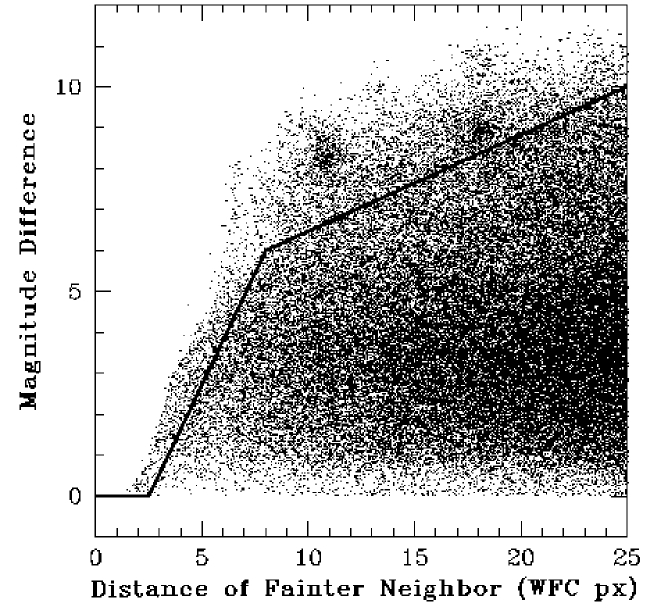
Figure 1.— Distribution of neighbors found around saturated stars in the GO-9028 F475W exposures used to construct the master frame. Each point represents a fainter neighbor of a saturated star and is plotted at the appropriate distance and magnitude offset from the main star. PSF artifacts show up as very faint objects relatively close to the star. All points above this line are considered to be potential artifacts. Some real stars are necessarily rejected as well, but in a very regular way so that completeness can be defined well.

2.2.2 Finding the Cluster Center

The ACS/WFC images provide us the widest, the most uniform, and the deepest survey to date of the central regions of 47 Tuc. Previous images taken by WFPC2 have a very asymmetric and non-uniform coverage, due to the lop-sided shape of the WFPC2 footprint and the gaps between the chips. By contrast, the dithered set of WFC images have essentially uniform coverage out to a radius of about 100″, which is nearly five core radii. These data therefore permit us the best determination to date of the cluster center. Indeed, given the high degree of completeness in the present star counts, it is difficult to imagine any significant improvement in the near future.

Note that a determination of the center from star counts should not depend on incompleteness corrections, provided of course that incompleteness is a function only of stellar magnitude and clustercentric radius. Nor should mass segregation enter the problem, so long as the stellar distribution is radially symmetric. Thus, in determining the center we work directly with our master star list, making no attempt to correct for either of these effects.

We begin with our list of 114,973 stars after culling faint neighbors (possible PSF artifacts). For each star we have a position $(x,y)$ in the reference-frame coordinate system, rotated in order to align the $y$ axis roughly with North. Next, an array of trial centers $(x_{0},y_{0})$ is defined, and for each trial center in turn we find all the stars within a radius of 1500 WFC pixels (75″) from that center. We then divide these stars into sixteen, $22.5^{\circ}$-wide pie wedges—shown schematically in the left panel of Figure 2—and use two tests to compare the distributions of stars in the eight distinct pairs of opposing wedges.

In the first test, we look at the difference in the total number of stars between the members of the opposing-wedge pairs defined by each $(x_{0},y_{0})$ in our pre-defined array of trial centers, and we form a “quality-of-fit” statistic as the sum of the differences over the eight wedge pairs. The coordinates which minimize this statistic then define a “median” estimate of the cluster center. The middle panel of Figure 2 shows a contour plot of the sum of differences for a 3″$\times$3″ subgrid of trial centers, with $(0,0)$ corresponding to the best center ultimately implied by this method (the conversion to calibrated right ascension and declination is discussed below).

The second test is to generate the cumulative radial distribution for stars within each of the sixteen wedges for any specified $(x_{0},y_{0})$. We then find the absolute value of the integrated difference between the radial distributions in any two opposing wedges, and define a quality-of-fit statistic as the sum of these absolute differences over the eight wedge pairs. The right panel of Figure 2 shows a contour plot of this statistic over a grid of trial centers, with $(0,0)$ again corresponding to the best-estimate coordinates which minimize the statistic.

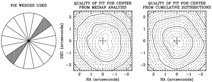
Figure 2.— Left: a shematic illustrating the wedges used to home-in on a cluster center; see text. Middle: contours of equal quality-of-fit statistic for determining the center using a “median” analysis, i.e., by comparing the total numbers of stars in pairs of opposing wedges. Right: contours of equal quality-of-fit statistic for determining the center using the cumulative radial distributions of stars in opposing wedges. In the middle and right panels, dotted contours represent changes of 20% in the quantity plotted. Errorbars represent the estimated uncertainty in the center.

Table 3Stars Used for Astrometric Calibration, and the Resulting Cluster Center

Point/Star	Master Frame ID	F475W	$x_{\rm raw}$	$y_{\rm raw}$	$\Delta$RA	$\Delta$Dec	RA (J2000)	Dec (J2000)
			[pixels]		[arcsec]		[hh:mm:ss]	[dd:mm:ss]
(1)	(2)	(3)	(4)	(5)	(6)	(7)	(8)	(9)
$\alpha$	M052296	13.6	1991	415	$-4.532$	$-5.983$	00:24:04.69$\pm$0.10	$-$72:04:58.58$\pm$0.12
$\beta$	M060833	14.3	1961	239	$-4.924$	$+2.935$	00:24:04.61$\pm$0.10	$-$72:04:49.69$\pm$0.11
$\gamma$	M061604	13.8	2163	182	$+5.180$	$+3.720$	00:24:06.79$\pm$0.10	$-$72:04:48.90$\pm$0.11
$\delta$	M056400	13.6	2208	281	$+6.809$	$-1.665$	00:24:07.15$\pm$0.11	$-$72:04:54.25$\pm$0.11
$\epsilon$	M056630	12.9	2013	319	$-2.903$	$-1.413$	00:24:05.04$\pm$0.11	$-$72:04:54.08$\pm$0.11
$\zeta$	M004529	14.2	2113	812	$-6.731$	$-74.669$	00:24:04.21$\pm$0.11	$-$72:06:07.29$\pm$0.10
$\eta$	M034527	13.4	3380	545	$+62.662$	$-26.247$	00:24:19.25$\pm$0.10	$-$72:05:18.77$\pm$0.12
Center	$\cdots$	$\cdots$	2066	277	$0.000$	$0.000$	00:24:05.67$\pm$0.07	$-$72:04:52.62$\pm$0.26

Note. — Key to columns: Column (1)—Label for the star in Fig. 3. See text for the distinction between stars $\alpha$, $\beta$, $\gamma$, $\delta$, and $\epsilon$ vs. stars $\zeta$ and $\eta$. Column (2)—Stellar ID on the sequential numbering system for the full master-frame star list of Table 4. Column (3)—Calibrated F475W magnitude. Column (4)—“Raw” $x$ position, in pixels, in the top chip (WFC1) of the j8cd01a9q_flt frame from program GO-9028. Column (5)—“Raw” $y$ position, in pixels, in the top chip (WFC1) of the j8cd01a9q_flt frame from program GO-9028. Column (6)—RA offset in arcsec (positive Eastward) from the cluster center in the master-frame system. Column (7)—Dec offset in arcsec (positive Northward) from the cluster center in the master-frame system. Column (8)—Calibrated, absolute right ascension. Column (9)—Calibrated, absolute declination.

Figure 3.— Left: stars in a 20″$\times$20″ field about our cluster center. Point size is correlated with F475W magnitude. The 5 stars used in the absolute calibration are indicated (see Table 3), as are the cluster centers estimated by Guhathakurta et al. (1992) and Calzetti et al. (1993) . Right: a close up of the inner 4″$\times$4″. The uncertainty in the center is about $\pm 0\farcs 25$ in each coordinate.

These two approaches give quite consistent positions for the cluster center. To get an idea of the accuracy of our center, we again take eight pairs of opposing wedges. For each pair, we find the location along the wedge axis that minimizes the difference between the cumulative radial distributions for the two wedges independently of any others. This yields eight estimates of the center along different axes using independent samples of stars. From the scatter among these independent estimates, we find that our final center is good (in the master-frame coordinate system) to about $\pm$5 WFC pixels (or $\simeq 0\farcs 25$) in both directions. This uncertainty is indicated by the errorbars at $(0,0)$ in the middle and right-hand panels of Figure 2.

2.2.3 Astrometric Calibration

We now have a position for the cluster center in the reference frame, which is based on the distortion-corrected and rotated frame of the first image of GO-9028. In order to transform the Master-frame positions into absolute RA and Dec, we used the image header information from several WFPC2 images (u2ty0201t, u2vo0101t, u4f40101r, and u5jm120dr) to obtain absolute positions for seven stars—five stars at the center and two stars in the outskirts. These four images were taken at different pointings and orientations, so they should all use different guide stars and give independent estimates of the absolute coordinates.

Table 3 gives details of these seven stars. First are their IDs in our master star list and calibrated F475W magnitudes (both of which items are described in general below). Following this are the stars’ locations in the master frame, both in terms of pixel positions and in terms of relative RA and Dec offsets from the cluster center determined in §2.2.2. Then we list the average absolute RA and Dec (J2000) obtained from the header information in the four WFPC2 images. Combining the absolute positions of the five central stars with their relative offsets in the reference frame then sets the absolute astrometric zeropoint of our master-frame system. The two outer stars $\zeta$ and $\eta$ are used to fix the orientation angle. As is also stated in the bottom line of Table 3, the absolute position of the cluster center is

$$\begin{array}[]{rcl}{\rm RA(J2000)}&=&~{}~{}00^{\rm h}\,24^{\rm m}\,05\fs 67\,\pm 0\fs 07\\ {\rm Dec(J2000)}&=&-72^{\circ}\,04^{\prime}\,52\farcs 62\,\pm 0\farcs 26\ ,\end{array}$$ (1)

where the uncertainties come from the averaging of the five stars and essentially reflect the $\pm 0\farcs 25$ internal uncertainty in the uncalibrated master-frame coordinates of the cluster center. This absolute calibration should be good to about 0.1 arcsecond throughout our $\sim$3′$\times$3′ master field, although we note that it may ultimately suffer from a small ($\sim$1″) inaccuracy if the positional errors of the HST guide stars for the WFPC2 frames we have used are correlated (see Taff et al., 1990).

The position of our adopted center is intermediate to those determined by Guhathakurta et al. (1992) and Calzetti et al. (1993). This is illustrated in Figure 3, the left panel of which shows a 20″$\times$20″ region about our adopted center with the 5 central reference stars in Table 3 marked. Our star $\epsilon$ is the star that Guhathakurta et al. used as a reference position (their star E). Our absolute coordinate for this star differs from theirs by about 1.5 arcseconds. The center position as estimated by Guhathakurta et al. is labeled with a “G,” placed at the position they report relative to star $\epsilon$ (not at the absolute coordinates given in their paper). We also mark the center found by Calzetti et al. with a “C.” Finally, the right panel of Figure 3 shows a close-up of the 4″$\times$4″ box around our center.

2.2.4 F475W Photometry

In the course of fitting PSFs to find positions, we also computed the average F475W fluxes of stars in the master frame. These fluxes include a spatially-dependent correction, of order $\sim 3\%$, for the fact that the ACS flat fields were designed to preserve surface-brightness rather than flux (Anderson 2006, ACS ISR in preparation). However, they were calculated from only the inner 5$\times$5 pixels around each stellar peak, and they correspond to a 60-second exposure. To calibrate the photometry, we must turn this flux into that which would be measured through the standard “infinite” aperture of 5 arcseconds (100 WFC pixels) in 1 second. We first compute the ratio of our measured flux to the flux contained within 10 pixels, or 0$\farcs$5. This ratio is 1.238. The encircled energy curves in the ACS Handbook (Pavlovsky et al., 2005) then show that 92.5% of the light should be contained within this radius. Thus, we scaled all our fluxes by a net factor of 1.339 upward and then divided by 60 (seconds) before adding the VEGAMAG zeropoint of 26.168 (De Marchi et al., 2004) to obtain a final, calibrated F475W magnitude for each star in the master list.

2.2.5 Completeness Fractions

The broad, uniform coverage of our WFC master frame also makes this a useful data set for constructing an accurate surface density profile for the cluster. We can detect almost all the stars there are, so it should be possible to come up with the definitive radial profile from the center out to nearly 5 core radii. There are, however, two issues that complicate the construction of any density profile from star counts in globular clusters: incompleteness and mass segregation. Mass segregation really just means that the density profile can differ, at least in principle, for stars in different mass (magnitude) ranges. It is a physical effect, separate from any instrumentation or data-reduction issues, and we discuss it briefly in §4 below, where we actually derive a density profile for the innermost parts of the cluster. Incompleteness, on the other hand, is a technical limitation of the observations themselves.

Incompleteness is always a joint function of both the images and the algorithm used to find stars in the images. It can arise from several sources. A particular star might not be found because (1) it is too close to a brighter neighbor and is not bright enough to generate its own peak in the image; (2) it could land on a defect in the chip or it could be hit by a cosmic ray; or (3) it could be close to the background and not bright enough to generate a peak above the noise. The fact that we have generated our list from many observations all at different pointings saves us from (2). And since the stars we analyze in this paper are always several magnitudes brighter than the faintest stars that can be detected in the master frame, issue (3) is not important for us. The first source of incompleteness (bright-star crowding) is the only thing we need to concern ourselves with here.

The usual strategy for evaluating incompleteness involves applying a set data-reduction procedure to a large number of artificially generated data sets. This is a rather daunting prospect in our case, and we have instead addressed the problem directly from the algorithm we used in §2.2.1 to identify (likely) non-stellar artifacts in our original list of 129,733 PSF peaks in the master frame.

First, we used the ACS images from program GO-9028 to create a circular image of the region $R\leq 150\arcsec$, with a uniform pixel size of $0\farcs 05$ pixel^-1. (Note that this reference image completely contains the master field itself, which is non-circular and measures only $\simeq 3\arcmin$ on a side. This is because we required a point to be covered by at least 7 ACS pointings to contribute to the master star list, but only one was sufficient to build the circular mosaic.) We then went pixel by pixel through the intersection of this circular frame with our master field, made a list of all stars found by our PSF-fitting within a 25-pixel ($1\farcs 25$) radius from each point, and recorded the faintest magnitude, $m_{\rm max}$, of the stars which could have survived the artifact-purging procedure of §2.2.1 and Figure 1. This yields an estimate of the limiting magnitude at every pixel in our master frame.

Given the limiting $m_{\rm max}$ at every point in our field, we calculated a “completeness fraction” for every star in the master list individually. Knowing the position $(x_{*},y_{*})$ and magnitude $m_{*}$ of each star in the list, we looked at the values of $m_{\rm max}$ at all points within 100 pixels ($=5\arcsec$) of $(x_{*},y_{*})$ and counted the number of pixels for which $m_{\rm max}<m_{*}$. That is, we computed the fraction $f\in[0,1]$ of the local area around each star where an identical star could fall but be discounted as unreliable by our criterion in §2.2.1 (or not be detected at all). The local completeness fraction at $(x_{*},y_{*},m_{*})$ is then just $c\equiv(1-f)$.

With $c$ defined pointwise in this way, every star in our master list is interpreted as representing $1/c$ actual stars, and corrected density profiles follow simply from the sums of $1/c$ over all points within specified areas on the sky. Again, we actually construct such a profile in §4.

2.2.6 Image of the Central Regions and the Final Star List

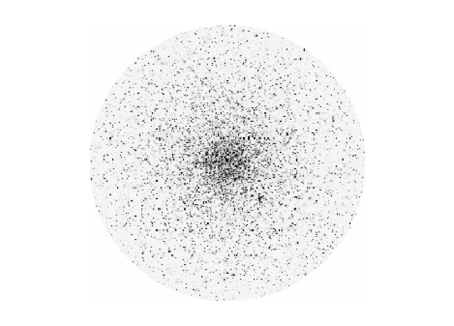
Figure 4.— ACS-based image of the central $R\leq 150\arcsec$ in 47 Tuc, inside of which we identify stars for the unbiased master list of Table 4. The image is available in .fits format from the online edition of the Astrophysical Journal. Pixel size in the online image is 0$\farcs$05 per pixel, and coordinates are defined with the cluster center at $(x,y)=(3001,3001)$ px. North is up and East is to the left.

As was mentioned just above, as part of our estimation of completeness fractions we constructed a meta-image of the innermost $R\leq 150\arcsec$ from the center of 47 Tuc. This convenient reference image, 47TucMaster.fits, oriented in the usual North-up, East-left way, is available through the online edition of the Astrophysical Journal. A low-resolution version of it is shown in Figure 4.

Table 4 finally presents all important information on the 129,733 coincident PSF peaks in our master field, which is fully contained in the circular area of the meta-image. (A sample of Table 4 can be found at the end of this preprint.) Only 114,973 of these peaks can be said confidently to be bona fide stars, but to be comprehensive, we have here retained (and flagged) the 14,760 peaks which could be PSF artifacts according to §2.2.1. The table gives the offset of each detection from the cluster center in arcseconds; the calibrated F475W magnitude; the absolute RA and Dec in real and celestial formats; the faintest magnitude a star at each position could have and still be found; a flag indicating whether the star survives the artifact purging; the local completeness fraction for the brightness and position of each star; a serial ID number; and $(x,y)$ coordinates in both our meta-image and the original image of the ACS/GO-9028 central pointing.

The absolute astrometric calibration of Table 4 should be good to about 0$\farcs$1, but the relative positions should be much better than this—particularly for bright, unsaturated stars and those with small separations, for which we estimate an accuracy of $\sim$0$\farcs$001. Of course, all the positions refer specifically to the epoch (2002.26) of the GO-9028 data set.

2.3. Reducing Images from Multiple Epochs

With a well-defined reference frame in hand, the next step toward deriving proper motions is to measure the positions of stars in individual images taken at different epochs and transform these into the master coordinate system. We began this task by measuring each star in each data set in Table 2 with an appropriate PSF, derived according to the method of Anderson & King (2000). For the ACS-WFC observations, we used a single PSF to treat the entire 2-chip association. We also used a single PSF for the entire ACS-HRC chip. The PSF does vary significantly with position over the ACS, but our data were reduced before the methods of Anderson & King (2006) were developed to deal with this. Nevertheless, Anderson (2002) shows that the biggest effect of this variation on astrometry is a small bias of 0.01 pixel in the positions. Since all our images are well-dithered, this error averages out and is included in the internal uncertainties for the positions. The constant-PSF assumption can also introduce systematic errors of up to 0.03 magnitudes in the photometry, but this is not of concern to us here.

All the raw measured positions were corrected for distortion using the prescriptions in Anderson & King (2003b) for WFPC2 data and Anderson (2006, in preparation) for ACS data. These corrections include the global and fine-scale distortion corrections, as well as a correction for the 68th-row defect. Charge-transfer inefficiency should not be an issue, as the background is relatively high in the images that we have used.

It was then necessary to combine all the observations of each star in the multiple pointings at each epoch. In all cases we adopted the centermost pointing as the “fiducial” frame for each epoch, and used general 6-parameter linear transformations (along the lines of those described in eq. [2] below) to transform positions from the individual, distortion-corrected pointings for that epoch into the central frame. In finding these transformations for WFPC2 images, we treated the PC chip and the three WF chips independently of the others; for the ACS images, the HRC chip and two WF chips were likewise considered independently. In this way, we found an average position for each star in each of 27 chip-epoch combinations. The standard deviation of a star’s position in the independent pointings at each epoch defines the uncertainty in $x$ and $y$ locations.

At this point we examined the errors in the stars’ positions as a function of their flux at each epoch in order to define a criterion to define which stars were well measured and which were not well measured within each data set. Figure 5 shows a plot of the position errors as a function of the instrumental magnitude $-2.5{\rm log}_{10}[N_{DN}]$ for some sample chip-epoch combinations. We drew the fiducial lines shown in Figure 5 to distinguish well measured from poorly measured stars; only stars falling below these lines in any of the data sets were retained for any further analysis. In addition to this, we discarded all stars found within the pyramid-affected region of any of the WFPC2 chips (ie., any at chip coordinates $x<100$ or $y<100$). We finally rejected any saturated bright stars from the star list for every data set.

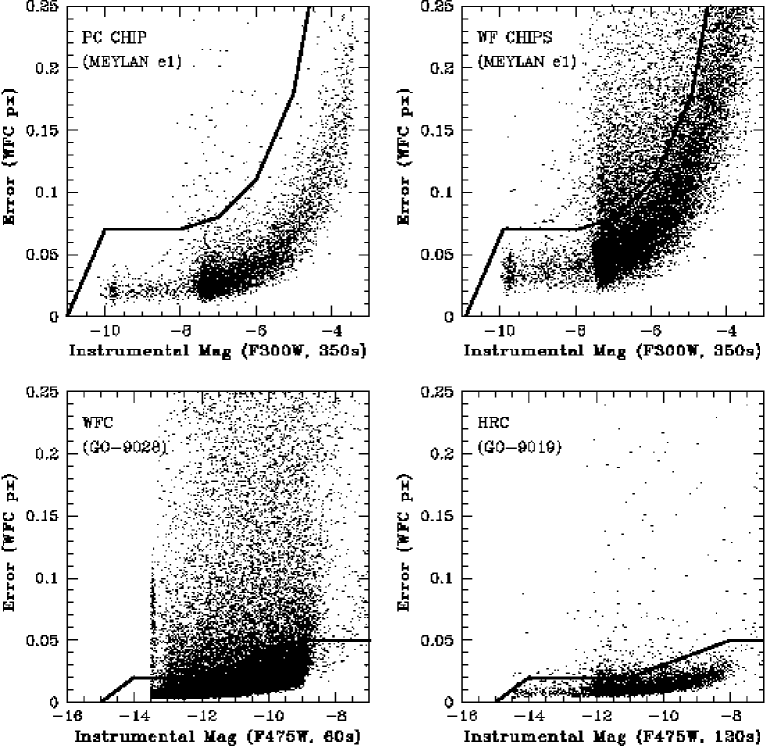
Figure 5.— Illustration of the criteria defining stars, on the various chips of different detectors, with positions that are “well-measured” enough to be used in deriving proper motions. Examples are shown at one epoch for each of the PC and WF chips on the WFPC2, and the WFC chips and HRC chip of the ACS. The discriminating lines drawn are applied to the list of positions and fluxes of all stars found at every epoch on each chip, with any detections falling above the appropriate line discarded as too uncertain to contribute meaningfully to the determination of a proper motion. The horizontal axes are given here in instrumental magnitudes to indicate the relationship between positional error and raw S/N. The location of the subgiant branch in 47 Tuc (calibrated $V\simeq 17.2$; cf. Fig. 10) is clear from the sharp increase in the density of points in each panel.

This left us with an average position, including uncertainties, and a flux for every star that we deemed well measured in each chip of each data set. The positions were still in the distortion-corrected coordinate systems of the individual epochs, however, and needed next to be transformed into the system defined by our master frame.

We should note explicitly here that the GO-9028 WFC data (epoch 2002.26) were subjected to the above analyses (and to the coordinate transformations described next) in exactly the same way as were any of the other epochs in Table 2—even though the master frame in §2.2 was itself defined using data from this epoch. This is because in constructing the master frame we used only 13 images from the 2002.26 WFC set of 20 and made no effort to impose any “quality control” on the stellar positions or magnitudes. However, any given star in the master list could, in principle, be observed in one or more of the seven other pointings at this epoch; or alternately its position might be so poorly constrained (relative to the criterion illustrated in Figure 5) that it is not useful for proper-motion measurements. Thus, to make optimal use of the GO-9028 WFC data requires that they be re-analyzed in parallel with the other epochs, with the master frame viewed simply as an externally imposed construct.

2.3.1 Linking with the Master System

The transformation into our master coordinate system is non-trivial. Given the small proper-motion dispersion in 47 Tuc (see Table 1) and our short ($\lesssim 7$ year) time baseline, we need to resolve displacements of order 0$\farcs$001 and less for the stars in our sample. The pointing of HST is good to only 0$\farcs$1 at best, however, and thus we cannot transform our positions to an absolute frame with anywhere near the accuracy required.

The only information we have about how the coordinate system of one frame is related to that of any other comes from the positions of stars that are common to both frames. Each observation typically has thousands of stars in common with the master frame. Once these stars are matched up, the two sets of positions can be used to define a linear transformation from one coordinate system to the other. Specifically, if we have a list of positions $\{x_{i},y_{i};i=1,\dots,{\cal N}\}$ for ${\cal N}$ stars at some epoch, and a list $\{X_{i},Y_{i}\}$ for the same stars in the master frame, then we specify

$$\begin{array}[]{lll}X_{i}&=&A\cdot(x_{i}-x_{0})+B\cdot(y_{i}-y_{0})+X_{0}\\ Y_{i}&=&C\cdot(x_{i}-x_{0})+D\cdot(y_{i}-y_{0})+Y_{0}\ ,\end{array}$$ (2)

for constants $A$, $B$, $C$, $D$, and $(x_{0},y_{0})$, $(X_{0},Y_{0})$ to be determined. It may look like there are eight free parameters in this transformation, but in fact we have the freedom to pick the zeropoint offset in one system. In particular, if we choose ($x_{0}$,$y_{0}$) to be the centroid of the ${\cal N}$ matched stars in the non-master frame, then ($X_{0}$,$Y_{0}$) is necessarily the centroid of the group in the Master system. With these set, then, standard least-squares regression can be applied to solve for the linear terms $A$, $B$, $C$, and $D$ from the $2{\cal N}$ observed pairs of coordinates. Our last concern is the question of how many stars should be used to do this.

2.3.2 Local Transformations

If we were to use all the stars in common between the master system and the data from any other epoch, the solution of equation (2) would correspond to the best global transformation between the two coordinate systems. Unfortunately, such a chip-wide solution may not give the best transformation for a given point. In particular, although all of our frames have been distortion-corrected, any residual distortions will introduce systematic errors in a global transformation. Such distortion errors tend to be cumulative, i.e., they are larger for stars that are farther apart. As a result, the distance between two nearby stars can be measured much more accurately than the distance between stars at different corners of a chip. We therefore decided to perform more local transformations, using smaller groups of relatively nearby stars to define different transformations at different positions in an observed frame. Such a scheme may sound computer intensive, but it is straightforward enough to implement and is not, in fact, exceedingly slow. Given that we will never be able to remove distortion perfectly, this is a useful way to minimize its effect on our results.

Two sources of error influence the choice of the number ${\cal N}_{\rm trans}$ of stars to use in solving the system of equations (2) for local transformations. First, the positions $\{x_{i},y_{i}\}$ and $\{X_{i},Y_{i}\}$ themselves are obviously subject to some uncertainty. If $\Delta$ denotes a representative value of this uncertainty, then the average transformation is fundamentally uncertain at a level $\sim\Delta/\sqrt{{\cal N}_{\rm trans}}$, which suggests that we would like ${\cal N}_{\rm trans}$ to be as large as possible. Second, the uncorrected residual distortion introduces appreciable systematic error if the “nearby” stars used to define the local transformation at any point come from too far away. This implies that we would like ${\cal N}_{\rm trans}$ to be as small as possible.

After some experimentation, we found that a reasonable compromise between these opposing tendencies was reached with ${\cal N}_{\rm trans}=45$ for our data. In practice, we took a single star from the list of well-measured positions at one epoch; found this target star’s nearest 55 neighbors; and matched these neighbors to positions in the master frame. We then used these 55 pairs of coordinates (not including the target star itself) to solve for the coefficients in equation (2); discarded the 10 stars which deviated most from the solution; and re-solved for the transformation using the 45 remaining stars. This was then used to transform the original, target star only into the reference frame. These steps were repeated for every well-measured star in the combined frame for each of our ten epochs, until we had measurements of RA and Dec position (relative to the cluster center) vs. time for all stars in a single, unified coordinate system.

We also performed this procedure using ${\cal N}_{\rm trans}=20$ and ${\cal N}_{\rm trans}=100$ and did not find significant differences, in general, from our results with ${\cal N}_{\rm trans}=45$. However, the lower number is approaching the limit of what we feel comfortable with in terms of vulnerability to small-number statistics, while the higher number is coming close to bringing in too-distant neighbors that could well be affected by uncorrected distortion errors.

There is another, somewhat more subtle source of error in our local transformations, which comes from the fact that all the stars are physically moving with respect to each other from one epoch to the next. Thus, even if a star’s position could be measured perfectly in every image, it is impossible to associate its location $(x,y)$ at some epoch perfectly with its position $(X,Y)$ in the master frame using a finite network of ${\cal N}_{\rm trans}$ moving neighbors. Put another way, any one network of neighbor stars might in fact have a real net motion relative to the cluster center, but our approach assumes that all such network motions are identically zero. This error gets averaged away over many networks, of course, so that the mean velocity we estimate for any group of stars will be unbiased. However, any estimate of the velocity dispersion, $\sigma$, is affected. Details of how we correct for this are given in Appendix A, which also discusses the correction of velocity dispersion for unequal measurement errors. Here we simply note that the net effect of the local-transformation error is an artificial inflation of the intrinsic stellar $\sigma$ by a factor of $(1+1/{\cal N}_{\rm trans})^{1/2}$, or about 1.011 for our chosen ${\cal N}_{\rm trans}=45$.

2.3.3 $V$- and $U$-Band Photometry

In addition to calibrated F475W photometry for all stars in our master field (§2.2.4), we have obtained calibrated $V$-band and F300W (roughly $U$-band) magnitudes for the subset of stars falling in the WFPC2 field of the original Meylan exposures (GO-5912, GO-6467, GO-7503; see Table 2, and note that $V$ exposures were also taken as part of these programs for photometric purposes only). As we will describe below, all stars for which we have derived proper motions were required to be detected in at least one of these three early epochs, and thus the full proper-motion sample has multicolor photometry. Although the standard $V$ bandpass is not substantially different from F475W, it is useful for relating our analyses to various ground-based observations, and to such things as theoretical stellar mass-luminosity relations. The shorter $U$-band photometry is useful for constructing a color-magnitude diagram of our velocity sample in order to investigate how CMD position might influence stellar kinematics.

$V$ photometry of the WFPC2 fields was calibrated against an HRC image of the core of 47 Tuc, using the VEGAMAG zeropoints in De Marchi et al. (2004). Star-by-star comparison with the calibrated photometry in Bica, Ortolani, & Barbuy (1994) shows agreement at the $\simeq 0.05$-mag level on average. The $U$ magnitudes were calibrated using the VEGAMAG zeropoint in the WFPC2 Data Handbook (Bagget et al., 2002). The main-sequence turn-off in our $V,(U-V)$ CMDs agrees well with that in Edmonds et al. (2003). We report the $V$ and $U$ photometry for our proper-motion stars in §3.1, where we now define the velocity sample.

3. Velocity Samples

Our multi-epoch astrometry data are most certainly not homogeneous. The 2002 epoch is relatively uniform, thanks to the even ACS/WFC coverage; but the earlier WFPC2 observations come from a different camera with different pointings, dithering patterns, fields of view, and resolutions. Thus, not every star in any one of the ten data sets of Table 2 can be found in all of the other nine.

In §3.1, we describe how we go from a heterogeneous sample of multi-epoch positions to a homogeneous sample of proper motions. We also examine the quality of the fits of straight lines to the position-vs.-time data, and the uncertainties in the final proper motions. In §3.2, we discuss the third component of velocity, that along the line of sight. Specifically, we have a large sample of ground-based radial velocities for stars in 47 Tuc, and we are interested in using these in conjunction with our proper-motion sample to obtain a kinematic estimate of the distance to the cluster (§6.3).

3.1. Proper Motions

To define a working sample of plane-of-sky velocities for kinematic analyses, we have chosen to work only with stars which are observed in at least three separate data sets prior to year 2000 (i.e., in three or four of the MEYLANe1, MEYLANe2, MEYLANe3, and GILLILU1 epochs in Table 2), and in at least one of the ACS data sets (any of the WFC or HRC fields) from 2002. Thus, we only derive proper motions for stars that have a minimum of four separate $(x,y,t)$ measurements spanning a minimum of about 4.4 years ($2002.26-1997.84=4.42$), and all derived velocities are effectively “tied down” by a precise ACS position measurement. In practice, most of our stars are in fact measured 6 or more times over the full 6.7-year timespan (1995.82–2002.56) of our epochs, and a good number do in fact appear in all 10 of the data sets listed in Table 2.

We further decided to include stars in the proper-motion sample only if they also appear in the master star list of §2.2—even if another ACS “epoch” might contain the star. Ultimately, this has some effect on the spatial distribution of the velocity sample. Figure 6 shows the RA and Dec offsets from our estimated cluster center for a subset of stars in our master list (the larger, rotated square field), and the positions of stars in the original MEYLAN epochs (the four smaller, more densely filled squares). Evidently, the combination of all our requirements gives us proper motions over a patch on the sky with roughly the familiar WFPC2 pattern, but with slightly larger gaps than normal between the chips (cf. §2.3) and with the outermost corners shaved off.

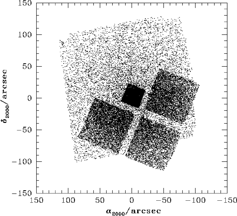
Figure 6.— Outline of the fields of view of our master star list (large square area; Table 4) derived from ACS program GO-9028, and of the original WFPC2 observations of GO-5912, 6467, and 7503. Only stars in the intersection of the two fields are retained for inclusion in the full proper-motion sample of Table 5.

We consider a star to be “observed” at any pre-2002 (WFPC2/MEYLAN or GILLIL) epoch only if it is detected in at least ten of the individual pointings/ditherings that went into that observation, and if it survives the culling based on position error vs. instrumental flux discussed around Figure 5 above. For any of the higher-precision, 2002 ACS observations, we take a star to be detected only if it is identified in at least four individual pointings/ditherings and if it again survives the appropriate culling by position error. These criteria are imposed to ensure that, whenever we include the measurement of a star’s position at any one epoch in our proper-motion determination, we also have enough information to estimate accurately the position uncertainty at that epoch.

The estimation of position uncertainties is of critical importance to the derivation of proper-motion uncertainties, and thus to the ultimate inference of intrinsic, error-corrected stellar kinematics. As was suggested in §2.3, we take a star’s position in any epoch to be the mean of the positions measured in the separate ditherings that were combined for that epoch and transformed into the master reference frame. The uncertainty is then simply the standard sample deviation of those independent multiple measurements. Note that we do not work with the uncertainty in the mean position (which would involve dividing the standard deviation by $\sqrt{N_{d}}$ for $N_{d}$ ditherings), because the theory of linear regression—which we use to derive velocities—actually requires that the square of the errorbars on the data be unbiased estimates of the variance in the position measurements.

Thus, given $(x,y)=(\alpha_{2000},\delta_{2000})$ positions and uncertainties as functions of time for any star that satisfies the minimum criteria just set out, we derive a plane-of-sky velocity in each direction by a standard, error-weighted least-squares fit of a straight line (e.g., Press et al., 1992, Section 15.2), allowing both the slope and the intercept to vary. This procedure automatically yields uncertainties in each component of velocity. The measurement-error distribution in each component of velocity for any single star will be Gaussian, with a mean of zero and a dispersion equal to the fitted least-squares errorbar, if the position measurement errors are similarly Gaussian distributed. We have assumed that this is the case.

The most important advantage of performing a weighted least-squares regression here is that it returns a $\chi^{2}$ value for each straight-line fit. Knowing the number of degrees of freedom in the fit ($=N_{e}-2$, where $4\leq N_{e}\leq 10$ is the number of independent epochs at which the star’s position was measured), it is then possible to calculate the probability that the $\chi^{2}$ of the fit could have occurred by chance if the true motion of the star were really linear (see Press et al., 1992). We can then make use of this to exercise some quality control over the proper motions, by excluding from kinematics analyses any stars with fitted velocities whose $\chi^{2}$ probabilities are lower than some specified threshold.

By fitting straight lines to our position-vs.-time data we are obviously assuming that the stars are moving at effectively constant velocity. To justify this in general, note that the characteristic gravitational acceleration in the core of 47 Tuc is of order (see Table 1, and §§4 and 6 below) $a_{0}\sim\sigma_{0}^{2}/r_{0}\sim(0.6\,{\rm mas\ yr}^{-1})^{2}/20\,{\rm arcsec}\sim 2\times 10^{-5}\,{\rm mas\ yr}^{-2}$. Even integrated over 7 years, the velocity change induced by such an acceleration is only $\sim 10^{-4}$ mas yr^-1, which is, as we shall see, a small fraction of the velocity uncertainties we infer. Of course, this does not exclude the possibility that some stars could be significantly accelerated by “nonthermal” processes such as stellar or black-hole encounters, or by virtue of being in tight, face-on binaries, or in some other way. Such stars will simply not be described well by straight-line motion, and the $\chi^{2}$ probabilities inferred from our weighted linear regression will reflect this fact. Thus, a low $P(\chi^{2})$ can reflect legitimately nonlinear data as well as simple “bad” measurements.

In all, we have 14,366 stars with RA and Dec positions measured to satisfactory precision in at least three pre-2000 epochs and at least one 2002 ACS epoch, and with measured $V$ and $U$ magnitudes (as described in §2.3.3). Table 5, which is published in its entirety in the electronic version of the Astrophysical Journal, contains the instantaneous J2000 RA and Dec positions in our master frame (epoch 2002.26) for all of these stars, expressed both in arcseconds relative to the cluster center determined in §2.2.2 (see also Table 1) and in absolute celestial coordinates. The F475W, $V$, and $U$ magnitudes of each star are also reported. The RA and Dec offsets (also in arcsec) from the nominal master-frame position, and their uncertainties, are then given for every epoch in which the star was detected. The proper-motion velocities and uncertainties implied by the weighted straight-line fitting to the offsets vs. time then follow, along with the $\chi^{2}$ values for the fits and the probabilities $P(\chi^{2})$ that these values could occur by chance if the motion is truly linear. We have not tabulated the intercepts of the linear fits, as these only reflect the choice of an arbitrary zeropoint in time and are of no physical interest in the constant-velocity case. (A sample of Table 5 can be found at the end of this preprint.)

Table 5 includes all stars for which we have estimated velocities, regardless of whether or not the $\chi^{2}$ values of the fits have “good” probabilities. We stress again that a reliable sample for kinematics work should exclude stars with very low $P(\chi^{2})$, but that some such stars could still be of interest for investigations of non–constant-velocity phenomena (which we do not pursue in this paper).

Two points should be noted regarding the connection between Table 5 and the larger master list of stars in Table 4. First, at the 2002.26 WFC-MEUR epoch in Table 5, the RA and Dec offsets from the absolute master-frame positions are consistent with 0 within the uncertainties for most stars, but they do not vanish exactly—even though this is the epoch that was used to construct the master frame. The reason for this is that the master list in §2.2 was defined using a very specific subset of the 20 individual exposures comprising the WFC-MEUR data set, while the relative positions found in §2.3 and used here to compute proper motions were allowed to come from different combinations of the 20 pointings. As a result, the transformations in the latter case cannot be expected in general to give positions identical to those in the master list, and the offsets for this epoch in Table 5 essentially reflect statistical noise. Second, there are some stars in Table 5 for which no offset at all is given at the WFC-MEUR epoch—an entry of “n/a” appears instead—even though all stars in the proper-motion table are guaranteed by construction to appear in the master list. In these cases, the uncertainties in the stars’ positions at the master-frame epoch were larger than acceptable according to our flux-based criterion defined in Figure 5 above, and thus these data were excluded from our fitting for proper motions.

Having derived proper motions for the best-measured stars in our field, we now describe the selection of a velocity subsample which is best suited for kinematics analyses. In particular, we can be more specific about how the $\chi^{2}$ probabilities in Table 5 are used to cull stars with particularly poor proper-motion measurements (or nonlinear motions), and we can quantify the distribution of the velocity uncertainties.

3.1.1 “Good” and “Bad” Proper Motions

Figure 7 shows plots of position (in milliarcseconds of RA and Dec offset from the master-frame position) vs. time (in years from the arbitrary zeropoint 1999.20) for two stars with relatively good proper-motion determinations. In the left panels is a bright star, near the cluster center, which has position measurements in Table 5 for 8 of our 10 data sets/epochs. In the right panels is a much fainter star, farther from the cluster center, which has fewer $(x,y,t)$ datapoints. In both cases, the fitted velocities $\mu_{\alpha}$ and $\mu_{\delta}$ in the RA and Dec directions are given in units of mas/yr, with $\mu_{\alpha}$ defined to be positive for Eastward motion. The $\chi^{2}$ probabilities for the linear fits of the two proper-motion components are also listed, showing that these data are fully consistent, within measurement error, with the basic assumption of constant velocity.

Figure 7.— Two examples of stars with good qualities of fit for straight-line proper motions: $P(\chi^{2})\geq 0.001$ in both velocity components. The ID numbers of the stars correspond to those in Tables 4 and 5. Plots such as these can be generated for any star in Table 5 using an SM macro available in the electronic edition of the Astrophysical Journal.

The much smaller position uncertainties in the most recent, ACS data relative to the pre-2002 (WFPC2) epochs are noteworthy. The right-hand panels particularly illustrate how the ACS epochs play a crucial role in defining the overall motions of our stars throughout the $\sim$7-year baseline of the observations. Indeed, if only the 4-year span of WFPC2 data had been fit to find a proper motion for the faint star in Figure 7, the RA component would have had the opposite sign (though with a larger errorbar) from that obtained when the ACS data are included. Evidently, relying on only a few epochs of astrometry, even with the HST, can lead to spurious proper motions for some individual stars.

Figure 8 next shows two stars with much less satisfactory proper-motion fits. Both stars here are fairly bright and near the cluster center, and both show more scatter about the best-fit linear velocity than is acceptable. On the left-hand side, the problem is primarily with the RA displacements in the upper panel, where the early (WFPC2) epochs do not match well onto the precise later (ACS) position measurements and $P(\chi^{2})$ is uncomfortably small. On the right-hand side, the scatter in both the RA and Dec motions is so large (relative especially to the small errorbars on the ACS positions at year $\simeq 2002$) that there is effectively no confidence that the best-fit constant velocity is an accurate representation of the data.

Figure 8.— Two examples of stars with poor qualities of fit for straight-line proper motions. With $P(\chi^{2})<0.001$ in one or both velocity components, stars such as these are not included in any working samples for kinematical analysis in this paper. They are, however, retained in Table 5. Plots such as these can be generated for any star in Table 5 using an SM macro available in the electronic edition of the Astrophysical Journal.

Plots like those in Figures 7 and 8 can be generated for any star from the data in Table 5, using an SM macro (pmdat.mon) that we have packaged and made available in the online edition of the Astrophysical Journal. After inspecting many such graphs and comparing the kinematics of samples of stars defined by imposing various lower limits on the allowed value of $P(\chi^{2})$ for the fitted velocities, we eventually decided to include in detailed analyses only stars which have

$$P(\chi^{2})\geq 0.001$$ (3)

for both RA and Dec components of proper motion. This criterion defines a velocity sample which cleanly excludes “bad” data such as those illustrated in Fig. 8 (as well as—again—potentially perfectly good data that are just nonlinear) and shows quite robust kinematics, in the sense that samples defined by revising the $P(\chi^{2})$ threshold in equation (3) moderately upward—even by as much as an order of magnitude—do not have significantly different statistical properties.

3.1.2 Proper-Motion Uncertainties

Figure 9 shows the distribution of uncertainties (least-squares errorbars) in the RA component of proper motion for stars in Table 5 which are brighter than $V<20$ and have $P(\chi^{2})\geq 0.001$ for the fitted values of both $\mu_{\alpha}$ and $\mu_{\delta}$. We have divided this subsample into three broad bins of projected clustercentric radius, $R$. It is immediately apparent that stars at $R>20\arcsec$ have systematically higher velocity errorbars, typically by factors of $\sim$2, than those at $R<20\arcsec$. This is because this radius is completely contained in the high-resolution, PC chip of the WFPC2 camera (see Figure 6), which affords higher precision in the measurement of (pre-2002) stellar positions than the WF chips which cover the larger radii in our field. From this alone it is clear that our velocity uncertainties correlate with clustercentric position.

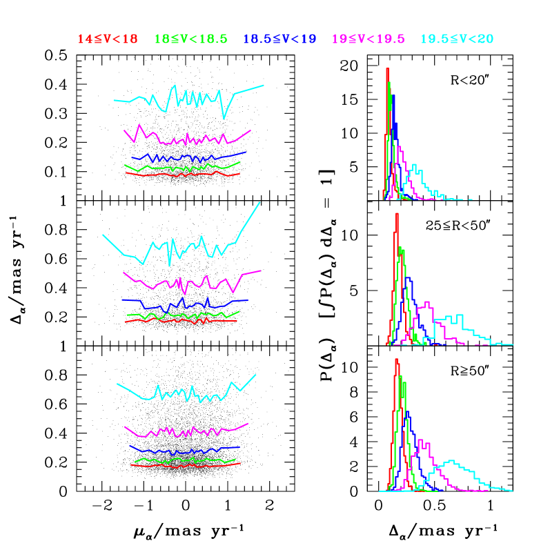
Figure 9.— Characterization of velocity uncertainties $\Delta_{\alpha}$ in the RA component of proper motion, $\mu_{\alpha}$. Left-hand panels are scatter plots of $\Delta_{\alpha}$, with colored lines connecting median values in bins of $\mu_{\alpha}$, for stars of different magnitudes. Right-hand panels are normalized histograms of the $\Delta_{\alpha}$ distributions, showing the tendency for the uncertainties to increase with $V$ magnitude and to be smallest in general at $R<20\arcsec$, corresponding to the region of the proper-motion field covered by the PC chip in the early WFPC2 images.

Panels on the left-hand side of Fig. 9 plot the proper-motion uncertainty $\Delta_{\alpha}$ against the velocity itself, $\mu_{\alpha}$. The colored lines, which correspond to different magnitude bins within each radial bin, connect the median $\Delta_{\alpha}$ errorbar in each of a number of discrete $\mu_{\alpha}$ bins. The right-hand panels then show the corresponding normalized histogram of velocity uncertainties in each radius/magnitude bin. These show that, for stars of a given magnitude, the distribution of $\Delta_{\alpha}$ not only peaks at smaller values for $R<20\arcsec$, but it is more sharply peaked there as well. Put another way, stars at the larger clustercentric radii have a stronger tail toward high velocity errorbars. Conversely—and quite naturally—at any fixed clustercentric radius, fainter stars always have larger average uncertainties and broader distributions. Indeed, the stars in the faintest magnitude bin illustrated here ($19.5\leq V<20$) have, at radii $R\geq 25\arcsec$, “typical” velocity errorbars of order 0.6 mas yr^-1 or more, which is comparable to the intrinsic velocity dispersion at the center of 47 Tuc (Table 1). Thus, stars of such faint magnitude will be of limited use for the statistical characterization of intrinsic cluster kinematics. Stars that are fainter still have even larger velocity uncertainties and are entirely useless in this context. Thus, we impose the magnitude limit

$$V<20$$ (4)

when choosing stars for any kinematics analysis. This is not to say that the velocities of individual faint stars are always unreliable—we shall see evidence to the contrary in §5.3—but only that their group properties are poorly constrained.

The distribution of velocity uncertainties for the Dec component of motion, $\mu_{\delta}$, is essentially identical, in all respects, to that shown for the RA component in Figure 9. The basic message of these plots is that, due to strong correlations with stellar magnitude and position, the errorbars on our fitted velocities cover a wide range of values and cannot be considered even approximately equal. Nor, in general, are they negligible relative to the intrinsic stellar motions. It is therefore important to account properly for the effects of measurement error on the observed proper-motion distribution and its moments (i.e., velocity dispersion). The details of this are discussed in Appendix A, where we also consider the statistical implications of the local-transformation approach to obtaining relative proper motions (cf. §2.3.2).

3.1.3 The Sample for Kinematics Analyses

Figure 10 shows color-magnitude diagrams and spatial distributions of the 14,366 stars with proper motions listed in Table 5, split into a sample in the left-hand panels which we consider useful for kinematics analyses (i.e., which comprises only stars satisfying both criteria in eqs. [3] and [4]) and a sample in the right-hand panels that we exclude from such work (i.e., which consists of stars with $P(\chi^{2})<0.001$ in either component of proper-motion velocity, and/or with magnitude $V\geq 20$).

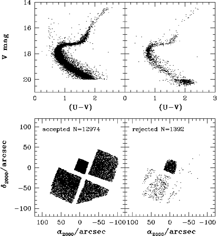
Figure 10.— Color-magnitude diagrams and spatial distributions of proper-motion stars which are used for subsequent kinematics work (left-hand panels), and those which are not (right-hand side). See text for details of the criteria by which stars are rejected.

The CMD of the upper left-hand panel exhibits a very well defined cluster sequence, including a red giant branch, a main-sequence turn-off at about the appropriate $V_{\rm TO}=17.65$ (Table 1), and even a small blue-straggler population. This is, in fact, not unexpected given that the foreground contamination in our small field (with an area of $\approx 3.5$–4 arcmin²) is expected to amount to perhaps $3\pm 2$ brighter than $V=21$ (from the foreground star density estimated by Ratnatunga & Bahcall 1985; see see Table 1). Note that we have no stars brighter than $V=14$ with measured velocities at all. Such stars were generally saturated in the 2002 ACS frames, and thus did not meet our selection criteria for the proper-motion sample.

The rejected stars in the right-hand panels of Figure 10 amount to only $\sim 10\%$ of the full sample in Table 5. 30% of them (417/1392) are rejected simply because they are fainter than $V=20$. The 975 others are rejected solely because they have a low $\chi^{2}$ probability for the linear fit to one or both components of their velocity. Of these, as Figure 10 suggests, the majority are brighter than $V=18.5$ and located within $R\leq 20\arcsec$ of the cluster center, where the stellar density is highest and crowding is most problematic.

It is important to check whether the rejection of these stars leads to significantly different kinematics for the “good” proper-motion sample than would have resulted if all stars were retained. Thus, in Figure 11 we show the cumulative distributions of RA and Dec velocities for stars with $V<18.5$ and $R\leq 20$, split into samples with $P(\chi^{2})\geq 0.001$ (accepted into a final kinematics sample) and $P(\chi^{2})<0.001$ (rejected). Kolmogorov-Smirnov tests applied to these indicate that the velocity distributions of the rejected stars are consistent with their having been drawn from the same parent distribution as the accepted stars. Thus, excluding the former from analysis does not give biased kinematics in the end but simply reduces the net uncertainty in our final results.

Figure 11.— Comparison of the cumulative RA and Dec velocity distributions for bright stars in the inner 20″ of our proper motion field, for the sample of stars with $P(\chi^{2})\geq 0.001$ in both proper-motion components, vs. those stars with $P(\chi^{2})<0.001$ in at least one component. In each panel, $P_{\rm KS}$ is the probability (from a Kolmogorov-Smirnov test) that the proper-motion distributions of the “good” and “bad” stars are in fact drawn from the same parent distribution. The high values of this statistic show that our results are not biased by excluding the poorest velocity fits from kinematical analysis.

Before going on to use our sample of 12,974 good proper motions to investigate these kinematics in detail, we first briefly describe some complementary line-of-sight velocity data that we use in §6.3 (only) to derive a kinematic distance to 47 Tuc.

3.2. Radial Velocities

3.2.1 The Data

The radial velocities used in this study come from two different instruments: the Geneva Observatory’s photoelectric spectrometer CORAVEL (Baranne, Mayor, & Poncet, 1979) mounted on the 1.5 m Danish telescope at Cerro La Silla, Chile, and the Rutgers Fabry-Perot spectrometer (e.g., Gebhardt et al., 1994) at CTIO. Details of the CORAVEL data are given by Mayor et al. (1983, 1984) and Meylan, Dubath, & Mayor (1991); typically, the measurements for relatively bright giants and subgiants have uncertainties of $\simeq 0.6$ km s^-1. The Fabry-Perot velocities include some previously published (Gebhardt et al., 1995), and some newly measured (Gebhardt et al. 2006, in preparation) from two runs at CTIO in 1995: one using the 1.5-meter telescope on 16–22 June 1995, and one with the 4-meter on 6–7 July 1995. The velocities normally have precisions of 1 km s^-1 or better, depending on the stellar magnitude and crowding.

All together, there are nearly 5,600 stars with CORAVEL and/or Fabry-Perot radial velocities, with Fabry-Perot contributing a large majority of the data. However, each of these samples covers a much larger area of 47 Tuc than does our proper-motion sample. We work here only with a much smaller subset of stars which lie within a radial distance of 105″ of the cluster center and thus overlap the proper-motion field (cf. Figure 10). In addition, we found it necessary to exclude from our analysis any Fabry-Perot stars fainter than the horizontal branch in 47 Tuc (which is also roughly the limiting magnitude of the CORAVEL data). This drastically reduces the sample size and thus requires some explanation.

The basic strategy of Fabry-Perot observations is described in Gebhardt et al. (1994, 1995, 1997). The idea is to scan an etalon across a strong absorption line (H$\alpha$ in our case) to build a small spectrum. The instrumental resolution of the Rutgers system is around 5000, and the FWHM of the H$\alpha$ line is larger than this. For the 4-meter observations of 47 Tuc, 21 steps across the H$\alpha$ line were used, while the 1.5-meter run observed two fields using 17 and 41 steps. The full range in all three cases was about 5Å. The exact wavelength coverage of any particular star depends on its location in the field, due to a wavelength gradient introduced by the Fabry-Perot. Given the full set of scans, DAOPHOT (Stetson, 1987) and ALLFRAME (Stetson, 1998) were used to determine the brightness of each star in the field. The scans were then combined to make a small spectrum, which was fitted for the H$\alpha$ velocity centroid.

There are particular advantages and disadvantages of this technique compared to the traditional slit échelle spectroscopy employed by CORAVEL. The latter provides large wavelength coverage, but it is obviously necessary to choose specific stars on which to place the slits. With this configuration, the observer has no control over what light goes down the slit, and neighboring stars can be be a severe contaminant in crowded regions. By contrast, Fabry-Perot spectroscopy provides only a small wavelength coverage but once the scans are completed, every star in the field produces a spectrum. This provides an enormous advantage in terms of the number of velocities that can be obtained. In principle, difficulties due to crowding should also be reduced since the use of DAOPHOT allows one to apportion the light appropriately in crowded regions, i.e., accurate photometry can be obtained for faint stars near bright ones.

Crowding inevitably remains an issue, however, with its main effect being a progressively stronger bias in the measured velocity dispersion at fainter magnitudes. If the spectrum of a faint star is affected by either a bright neighbor or the collective light of the bulk of unresolved cluster stars, the measured velocity is pulled closer to the cluster mean, and the velocity dispersion that follows is spuriously low. In the context of our work in §6.3, where we compare proper-motion to radial-velocity dispersions to estimate the distance to 47 Tuc, this effect would ultimately lead to a short value. There are two options for avoiding this. One is to remove the effect statistically, by using detailed simulations to define empirical, magnitude-dependent corrections for the stellar velocities. This approach is pursued by Gebhardt et al. (2006, in preparation). The other option is simply to make a magnitude cut in the velocity sample, keeping only those stars which are bright enough not to be significantly contaminated in the first place. This is what we have done here.

Figure 12 shows the distribution of the combined CORAVEL and Fabry-Perot radial velocities for stars in three bins of clustercentric radius. The left-hand panels include only stars with $11\leq V<14$, a magnitude range that has been well explored in previous radial-velocity studies, and which we have confirmed does not suffer significantly from the contamination problems just discussed. The limit $V\geq 11$ excludes only a handful of measured stars in this region of the cluster but is imposed to guard against radial-velocity “jitter” in the brightest cluster giants (Gunn & Griffin, 1979). The faint limit $V<14$ corresponds to the magnitude of the horizontal branch. The right-hand panels then include stars just slightly fainter than this, in the range $14\leq V<14.5$.

Figure 12.— Histograms of CORAVEL and Fabry-Perot radial velocities in the inner 105″ of 47 Tuc, comparable to the area covered by our proper-motion survey. Left-hand panels are for stars brighter than the cluster horizontal branch, and right-hand panels are for stars just 0.5 mag fainter. The sharp drop in the (error-corrected) dispersion $\sigma_{z}$ from the bright to the faint magnitudes—especially at the smaller clustercentric radii—signals a crowding-induced bias in the Fabry-Perot velocities.

We have calculated the error-corrected velocity dispersion $\sigma_{z}$ (see eq. [A7]) for the stars in each of the magnitude ranges and radial bins defined in Figure 12. These are listed in the appropriate panels of the figure, where we have also drawn (strictly for illustrative purposes) Gaussians with dispersions $\sigma_{z}$ on top of the velocity histograms. Comparing these results for the two magnitude bins at any given radius immediately shows the downward biasing of $\sigma_{z}$ caused by crowding. Comparing the different radii confirms this interpretation of the situation, since (1) the difference between $\sigma_{z}$ for the bright and faint samples decreases toward larger clustercentric radii, where the stellar densities are lower; and (2) the velocity dispersion at the smallest radii $R<25\arcsec$ for the fainter stars especially is dramatically (and unphysically) lower than that at larger $R$. Although $\sigma_{z}$ for the stars with $V<14$ is formally lower at $R<25\arcsec$ than in the range $25\arcsec\leq R<50\arcsec$, by some 0.7 km s^-1, the uncertainty in the calculated dispersion is also 0.7–0.8 km s^-1 in both radial ranges. Thus, the difference in this case is not highly significant and is likely a reflection of small-number statistics rather than serious contamination.

Given the results in Figure 12, we choose to include only stars brighter than the horizontal branch, $11\leq V<14$, in the radial-velocity sample used in this paper. There are only 419 such stars in the inner 105″ of 47 Tuc, and thus any kinematic estimate of the distance is fundamentally limited to a precision of no better than $(2\times 419)^{-1/2}\simeq 3.5\%$. Clearly, it is desireable to do better than this, and in principle it is possible to enlarge the radial-velocity sample by, say, applying position-dependent magnitude cuts to remove contaminated stars and/or using data from clustercentric radii beyond the proper-motion field. However, either of these things would require a sophisticated analysis of the Fabry-Perot data and an in-depth dynamical modeling that are well beyond the scope of this paper.

3.2.2 Overlap with the Proper-Motion Sample

Figure 13 shows the RA and Dec components of proper motion vs. stellar magnitude for our “good” proper-motion sample of §3.1.3 [i.e., those stars in Table 5 with $P(\chi^{2})\geq 0.001$ and $V<20$], and also for the combined CORAVEL and Fabry-Perot line-of-sight velocity sample in the inner $R<105\arcsec$ of 47 Tuc. Again, we do not make use here of any data at $V>14$ in the latter case, but Figure 13 emphasizes that radial velocities can indeed be measured for many such faint stars. The great potential of these data, if their systematic problems can be solved, is clear.

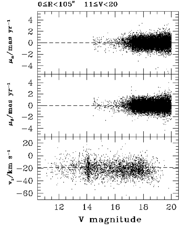
Figure 13.— Velocity vs. magnitude for stars in our “good” proper-motion sample [$V<20$ and $P(\chi^{2})\geq 0.001$ for both $\mu_{\alpha}$ and $\mu_{\delta}$; from Table 5], and for all stars at $R<105\arcsec$ in the CORAVEL and Fabry-Perot radial-velocity sample. Since the biasing problem illustrated in Figure 12 precludes the use of any line-of-sight velocities when $V>14$, we do not currently have a single star for which all three components of velocity have been reliably measured.

Figure 13 also illustrates the fact that there is currently not one star in 47 Tuc which has reliable measurements for all three components of its velocity. As was also mentioned in §3.1.3, stars brighter than $V=14$ were not measured in any ACS frames, and thus do not appear in our proper-motion sample; but fainter than this limit we cannot trust the radial-velocity measurements in general. As a result, only statistical comparisons of motions on the plane of the sky and along the line of sight are feasible at this point.

Finally, Figure 14 compares the spatial distribution of the 419 stars whose radial velocities can be used for a distance estimate (large points), to that of our good proper-motion sample (small dots, plotted for only a fraction of the 12,974 stars to outline the shape of the field). The circles drawn on this graph have radii of 25″ (which completely encloses the PC-chip area of the proper-motion field), 50″, 75″, and 100″. As we discuss further in §6.3, the obvious differences between the non-uniform spatial coverages of the two kinematics samples mean that some care must be used in properly comparing the measured velocity dispersions to derive a distance to the cluster.

Figure 14.— Comparison of the spatial distribution of our good proper-motion sample and the useable radial-velocity stars. All positions are plotted relative to the cluster center (§2.2.2), and for reference the large, dotted circles have been plotted with radii of 25″, 50″, 75″, and 100″.

4. Spatial Structure and a Model Velocity Distribution

To optimally explore the implications of the velocity data that we have assembled, we would like to relate them to a dynamical model for 47 Tuc. Ideally, this should be constrained by the spatial distribution of stars as a function of magnitude (mass) and allow for the possibilities of rotation, velocity anisotropy, axisymmetry (rather than sphericity), the presence of heavy stellar remnants, and so on. The proper construction of such a comprehensive, global model is clearly a large task that would involve bringing in more data than we have collected here (e.g., the spatial and velocity distributions of stars at radii beyond the $\simeq 100\arcsec$ extent of our proper-motion sample; information on the stellar luminosity function as a function of position in the cluster; etc.). Our much more modest goal in this paper is to try and extract as much model-independent information as possible from our proper motions, and simply to check whether they are broadly consistent with a very low-level description of the cluster.

The zeroth-order model we use as a reference point is the familiar single-mass, isotropic, modified isothermal sphere of King (1966). Note that Meylan (1988, 1989) has already fitted 47 Tuc with more realistic models of multimass and anisotropic clusters, but using only radial velocities and the surface-brightness profile of subgiants and giants as observational constraints. Thus, applying Meylan’s results as they are to assess fine details of our proper-motion data would not really be any more appropriate than using a single-mass and isotropic model (and re-fitting them would, as we’ve suggested, involve work beyond the scope of this paper). At any rate, Meylan’s models imply that velocity anisotropy is only important at large radii $R\gtrsim 500\arcsec$, i.e., in regions of the cluster not probed by our proper motions.

Similarly, Meylan & Mayor (1986) and Anderson & King (2003a) have quantified the rotation of 47 Tuc, using both line-of-sight velocities and proper motions. However, in the innermost $R\lesssim 100\arcsec$ covered by our new velocity data, rotation appears to be present only at the level of $\lesssim 3$ km s^-1, which is only a fraction of the velocity dispersion there (see Meylan & Mayor 1986, and §6.4 below). Thus, comparison of the proper-motion kinematics with a non-rotating and spherical model can still be profitable in this region.

In §4.1, then, we use our master star list from §2.2.6 to construct a new density profile for the brightest stars in the core of 47 Tuc, and combine this with wider-field, ground-based surface photometry to fit a King (1966) model to the cluster’s spatial structure. In §4.2 and Appendix B, we discuss the proper-motion velocity distribution predicted by such a model.

4.1. Density Profile of Turn-off Stars

The most important concern for us in constructing a surface-density profile from our master star list is the question of mass segregation. This involves massive stars (or heavy remnants) sinking toward the cluster center and following a more concentrated radial distribution than lower-mass stars, so we cannot really speak of a single density profile for the cluster. In fact, the data in Table 4 above could be used to explore mass segregation in some detail, but once again it is beyond the scope this paper. Some early work has been done by Paresce, de Marchi, & Jedrzejewski (1995), Anderson & King (1996), and Anderson (1997).

The best constraint on the spatial structure of 47 Tuc outside the core regions observed by HST is the $V$-band surface photometry collated from a variety of sources by Meylan (1988). The cluster light in this band is dominated by giants and subgiants, all of which have roughly the same (main-sequence turn-off) mass. Our immediate interest, then, is in defining an improved profile in the central region for stars of this mass only. The brightness of the main-sequence turn-off in 47 Tuc is $V=17.65$ (see Table 1), corresponding roughly to magnitude $17.8$ in the F475W bandpass for which our master star list has photometry. Thus, after first checking that the radial distribution does not vary significantly as a function of magnitude for stars brighter than the turn-off, we have used Table 4 to construct a single density profile for all stars with $m_{\rm F475W}\leq 17.8$. We emphasize that the full master star list has to be used for this, and not any sample of only proper-motion stars from Table 5, because the latter have a highly irregular distribution on the sky and a complicated (and unquantified) incompleteness as a function of magnitude and clustercentric position.

We first define a series of concentric circular annuli $\{R_{j}\}$, all contained entirely within the area of the master frame. The estimates $c_{i}$ of completeness percentage for individual stars in the master list (Column 10 of Table 4; see §2.2.5) are then used to calculate the density in each annulus: if there are ${\cal N}_{\rm raw}$ stars with $m_{\rm F475W}\leq 17.8$ in the range $R_{j}\leq R<R_{j+1}$, then the completeness-corrected number is ${\cal N}_{\rm cor}=\sum_{i=1}^{{\cal N}_{\rm raw}}(100/c_{i})$ and the net density follows as $\Sigma={\cal N}_{\rm cor}/\pi(R_{j+1}^{2}-R_{j}^{2})$. The results of this simple exercise are given in Table 6. Note, from comparison of the listed ${\cal N}_{\rm raw}$ and ${\cal N}_{\rm cor}$, that the corrections for incompleteness in this magnitude range are quite modest over our entire field. Also, no corrections are made for contamination by foreground or background stars, since the level of such contamination is negligible in this small area of the sky; see Table 1 again.

Table 6Density Profile of Cluster Stars With $F475W\leq 17.8$

Annulus	$R_{\rm eff}$	${\cal N}_{\rm raw}$	${\cal N}_{\rm cor}$	$\Sigma(R_{\rm eff})$
[arcsec]	[arcsec]			[arcmin-2]
0.00–1.00	0.707	11	11.601	$13294\pm 3903$
1.00–2.00	1.581	20	21.262	$8121\pm 1761$
2.00–3.00	2.550	58	62.564	$14339\pm 1813$
3.00–4.00	3.536	55	58.602	$9593\pm 1253$
4.00–5.00	4.528	74	79.081	$10069\pm 1132$
5.00–6.00	5.523	61	65.143	$6786\pm 841$
6.00–7.00	6.519	96	102.398	$9026\pm 892$
7.00–8.00	7.517	105	111.938	$8551\pm 808$
8.00–9.00	8.515	121	128.596	$8668\pm 764$
9.00–10.00	9.513	118	124.707	$7521\pm 674$
10.00–11.25	10.643	170	179.638	$7750\pm 578$
11.25–13.00	12.157	231	243.714	$6581\pm 422$
13.00–14.50	13.770	230	241.322	$6704\pm 432$
14.50–16.25	15.400	258	270.542	$5761\pm 350$
16.25–18.75	17.545	373	389.131	$5096\pm 258$
18.75–21.25	20.039	421	437.655	$5015\pm 240$
21.25–25.00	23.201	676	699.629	$4623\pm 175$
25.00–30.00	27.613	777	797.922	$3325\pm 118$
30.00–35.00	32.596	786	802.515	$2830\pm 100$
35.00–40.00	37.583	698	709.851	$2169\pm 81$
40.00–45.00	42.573	687	696.558	$1878\pm 71$
45.00–50.00	47.566	641	648.666	$1565\pm 61$
50.00–57.50	53.881	949	959.069	$1363\pm 44$
57.50–65.00	61.365	867	874.353	$1091\pm 37$
65.00–72.50	68.852	888	894.248	$993.7\pm 33.2$
72.50–82.50	77.661	988	993.452	$734.5\pm 23.3$

Note. — Number densities in last column are $\Sigma(R)\equiv{\cal N}_{\rm cor}/[\pi(R_{2}^{2}-R_{1}^{2})]$ with $R_{1}$ and $R_{2}$ the inner and outer radii of an annulus (Column 1), in units of arcmin. Uncertainty in $\Sigma(R)$ is $\sqrt{{\cal N}_{\rm cor}}/[\pi(R_{2}^{2}-R_{1}^{2})]$. To transform into $V$-band surface brightness on the scale of Meylan (1988) (uncorrected for reddening), set $\mu_{V}[{\rm mag\ arcsec^{-2}}]=(24.237\pm 0.021)-2.5\,\log(\Sigma/{\rm arcmin^{-2}})$.

It remains only to combine these star counts with the wider-field $V$-band surface photometry taken from Meylan (1988). We first define an effective radius for each annulus, $R_{{\rm eff},j}^{2}\equiv(R_{j}^{2}+R_{j+1}^{2})/2$. The number density at each $R_{\rm eff}$ is then converted to a surface brightness as $\mu(R_{{\rm eff},j})=C-2.5\,\log\Sigma(R_{{\rm eff},j})$, where $C$ is a constant determined by the overlap of our data with the calibrated Meylan photometry. In practice, we only use the ground-based surface brightnesses $\mu_{V}$ at clustercentric radii $R\geq 20\arcsec$ (to guard conservatively against any potential seeing-induced blurring of the central profile) and obtain $C$ as the median value of $[\mu_{V}+2.5\,\log\Sigma(R_{\rm eff})]$ for all of our data points with $20\arcsec\leq R_{\rm eff}\leq 70\arcsec$. We find that the new HST number counts are brought nicely onto the $V$-band surface-brightness scale of Meylan (1988) (uncorrected for reddening) with the transformation

$$\mu_{V}=(24.237\pm 0.021)-2.5\,\log(\Sigma/{\rm arcmin}^{-2})\ .$$ (5)

Figure 15 shows the composite surface-brightness profile for 47 Tuc. Open squares represent the data from Meylan (1988), while the filled circles correspond to our star counts after the application of equation (5). We have also plotted, as the open triangles, earlier HST-based number densities of turn-off stars from Howell, Guhathakurta, & Gilliland (2000, their Figure 4), transformed by $\mu_{V}=(14.927\pm 0.033)-2.5\,\log(\Sigma_{\rm HGG}/{\rm arcsec}^{-2})$ to give the best match to the ground-based surface photometry at $20\arcsec\leq R\leq 70\arcsec$. The agreement between the two HST data sets is very good overall, confirming the conclusion of Howell, Guhathakurta, & Gilliland (2000) that 47 Tuc has a smooth, well-defined, and reasonably large core that shows no sign of the cluster having undergone core collapse.

Figure 15.— $V$-band surface-brightness profile of 47 Tuc, constructed by combining the ground-based surface photometry compiled by Meylan (1988) at $R\geq 20\arcsec$, with HST star counts at $R\lesssim 100\arcsec$ from Howell, Guhathakurta, & Gilliland (2000) and our own master list (Table 4). Only stars brighter than the main-sequence turn-off were included in the HST number-density profiles, which were converted to $\mu_{V}$ as described in the text. The bold, dash-dot curve is the fit of a single-mass, isotropic, King (1966) model, with the parameters indicated (also listed in Table 1). This model only attempts to describe the cluster structure at small radii. The poor fit at $R\gtrsim 1000\arcsec$ is due to neglecting velocity anisotropy and multiple stellar masses, but the disagreement with $\mu_{V}$ in the extreme halo does not impact the core region $R<100\arcsec$ covered by our proper-motion data.

The dot-dash curve in Figure 15 is our fit of a single-mass, isotropic, King (1966) model to the combination of our data points with the brightness profile of Meylan (1988). Only data at $R<1100\arcsec$ were used to constrain the fit since, as we discussed above, we only require a good description of the central regions covered by our proper-motion data. Our best estimates of the core radius $r_{0}$, central surface brightness $\mu_{V,0}$, and concentration parameter $c\equiv\log(r_{t}/r_{0})$ (for $r_{t}$ the tidal radius of the model) are written on Figure 15 and also listed in Table 1 above. Note that the fitted $c=2.01$ corresponds to a dimensionless central potential $W_{0}=8.6$ (see Appendix B). We estimate uncertainties of about $\pm 25\%$ in $r_{0}$, $\pm 0.25$ mag in $\mu_{V,0}$, and $\pm 0.1$ dex in $c$ (or $\pm 0.4$ in $W_{0}$). (Note that these uncertainties are correlated, such that fits with higher $c$ tend to require smaller $r_{0}$ and brighter $\mu_{V,0}$.) Thus, while the new values of $r_{0}$ and $\mu_{V,0}$ here are formally slightly smaller and brighter than the “standard” values in the literature (e.g., Harris, 1996; Howell, Guhathakurta, & Gilliland, 2000), the differences are at the $\sim 1$-$\sigma$ level. Our core radius is in good agreement with the $r_{0}=21\arcsec$ recently derived by Mapelli et al. (2004), also from HST star counts.

Given our neglect of the data at large $R\geq 1100\arcsec$ when fitting the King (1966) model in Figure 15, its failure in these outermost parts of the cluster is not surprising. In fact, no single-mass and isotropic King model can satisfactorily fit the entire run of surface brightness throughout 47 Tuc. This is already well known and forms the basis of the multimass and anisotropic modeling of this cluster by Meylan (1988, 1989).

4.1.1 Effect of Mass Segregation

As we suggested above and will show explicitly in §6, a model that assumes velocity isotropy in order to give a description of the density distribution over radii $R\lesssim 1000\arcsec$ is appropriate enough as a benchmark in the discussion of our proper-motion observations at $R\lesssim 100\arcsec$. More worrisome in principle is the assumption of a single stellar mass and the implication that stars in any magnitude range should have a common spatial structure. This is patently untrue even in the core of a relaxed cluster; but even so, it turns out that the proper-motion stars in our case do not, in fact, span a particularly wide range in mass.

To assess this issue briefly, Table 7 summarizes a theoretical mass–$V$ magnitude relation for stars from 0.5–$0.9\,M_{\odot}$. In the second column of the table, the absolute magnitudes associated with $m_{*}\leq 0.8\,M_{\odot}$ are those calculated by Baraffe et al. (1998) for a 12.6-Gyr old cluster with ${\rm[M/H]}=-0.5$. For $0.8\,M_{\odot}<m_{*}<0.9\,M_{\odot}$ we have relied on the models of Bergbusch & VandenBerg (2001), as illustrated by Briley et al. (2004), for a 12-Gyr old cluster with ${\rm[Fe/H]}=-0.83$ and ${\rm[\alpha/Fe]}=+0.3$. The apparent $V$ magnitudes in the third column of Table 7 follow from $M_{V}$ given a reddening of $E(B-V)=0.04$ mag and an assumed heliocentric distance $D=4$ kpc to 47 Tuc (see Table 1, and §6.3 below). The simple formula on the bottom line, for $m_{*}$ as a function of $V$, is our own approximation. As §3.1 discussed in detail, our proper-motion sample is limited by the constraint $V<20$, which corresponds to stellar masses $0.65\,M_{\odot}\lesssim m_{*}\lesssim 0.9\,M_{\odot}$. The large majority of the stars for which we can meaningfully address kinematics questions differ in mass by $<20\%$ from the main-sequence turn-off and giant-branch stars ($V\lesssim 17.65$, so $m_{*}\simeq 0.85$–$0.9\,M_{\odot}$) for which we fit the King (1966) model in Figure 15.

King models with high concentration such as the one in Figure 15 are not substantially different, in their inner parts, from bounded (finite central density) isothermal spheres. Crude expectations for the relative density profiles at small radii for stars of different masses in 47 Tuc can therefore be obtained by considering models of two-component clusters in this idealized limit. Taff et al. (1975) show that two populations of stars with masses $m_{2}\geq m_{1}$ in an equilibrium isothermal sphere have density distributions related by $\rho_{2}(r)/\rho_{2}(0)=[\rho_{1}(r)/\rho_{1}(0)]^{m_{2}/m_{1}}$. As expected, then, $\rho_{2}(r)$ falls off more rapidly than $\rho_{1}(r)$ and the heavier stars are more strongly concentrated toward the center. To quantify this, note that the scale $r_{0}$ defined by King (1966, see our equation (B5) below) is, by construction, nearly equal to the radius at which the surface density of an isothermal sphere falls to half its central value. As a result, it is also related by a unique numerical factor to the radius at which the volume density is halved. Thus, we have calculated $\rho/\rho(0)$ and $[\rho/\rho(0)]^{m_{2}/m_{1}}$ vs. $(r/r_{0})$ for an isothermal sphere, for a range of fixed mass ratios, and located the dimensionless radii at which the dimensionless $\rho$ and $\rho^{m_{2}/m_{1}}$ fall (separately) to $1/2$. For modest values of $m_{2}/m_{1}$, the core radii of the two mass classes turn out to be related roughly by

$$r_{0,2}/r_{0,1}\simeq\left(m_{2}/m_{1}\right)^{-0.58}\ ,$$ (6)

accurate to better than 1% for $1\leq m_{2}/m_{1}\leq 3$ and in good agreement with the alternative approximation developed by Grindlay et al. (2002, their equation 5a).

Returning to 47 Tuc, we do not expect equation (6) to hold exactly; but in the absence of detailed modeling it is useful as an order-of-magnitude guide to the situation in the core region where all mass classes are expected to be nearly thermalized (with the velocity dispersion of each species scaling as $\sigma^{2}\sim m_{*}^{-1}$). For example, the core radius $r_{0}$ of the faintest stars in our proper-motion sample should be only slightly larger than that of the turn-off stars with $m_{*}\simeq 0.85\,M_{\odot}$: $(0.65/0.85)^{-0.58}=1.17$. Even the “average” cluster stars with $m_{*}\simeq 0.5\,M_{\odot}$ should be distributed with a scale radius differing by only $\sim 35\%$ [$(0.5/0.85)^{-0.58}=1.36$] from that of the density profile shown in Figure 15. We will refer back to this approximate relation on occasion below, when discussing various aspects of the velocity distribution of our proper-motion stars. First, we describe the expected form of this distribution for an isotropic and single-mass King-model cluster.

Table 7Stellar Mass-Luminosity Relation

$m_{*}/M_{\odot}$	$M_{V}$	$V=(M_{V}+13.13)$
0.9	$\lesssim$3.91	$\lesssim$17.00
0.8	$\lesssim$5.01	$\lesssim$18.14
0.7	$\lesssim$6.27	$\lesssim$19.40
0.6	$\lesssim$7.58	$\lesssim$20.71
0.5	$\lesssim$8.85	$\lesssim$21.98
$m_{*}/M_{\odot}\simeq 0.9\phantom{\ -0.081\,(V-17)}$		$V\lesssim 17.0$
$\phantom{m_{*}/M_{\odot}\ }\simeq 0.9-0.081\,(V-17)$		$V>17.0$

Note. — Based on the evolutionary models of Baraffe et al. (1998) and Bergbusch & VandenBerg (2001, see also ). Apparent magnitudes in Column (3) correspond to the absolute magnitudes in Column (2) for an assumed distance of $D=4.0$ kpc to 47 Tuc and a reddening of $E(B-V)=0.04$ mag.

4.2. Projected Velocity Distribution

As was noted above, the inner regions of King (1966) models with high concentrations (or central potentials) are dynamically quite similar to isothermal spheres. Given that our proper-motion sample covers only (parts of) the innermost $R\lesssim 5r_{0}$ in 47 Tuc, we first ask how different from Gaussian we might expect the observed velocity distribution to be. Very simple considerations suggest immediately that even for a sample of $\sim$10,000 stars the departure from Gaussianity is somewhat subtle.

First, King models are defined by a finite escape velocity at every radius in the cluster. If $W(r)=-\phi(r)/\sigma_{0}^{2}$, where $\phi(r)$ is the gravitational potential and $\sigma_{0}$ is a parameter closely related (though not equal) to the central velocity dispersion, then the model escape velocity at radius $r$ is $v_{\rm max}/\sigma_{0}=\sqrt{2W(r)}$, which is a monotonically decreasing function of radius (see Appendix B for more detail). A star moving outward from radius $r$ with velocity $v_{\rm max}(r)$ would just reach the cluster tidal radius with zero velocity. Our proper-motion field contains the center of 47 Tuc, where $W(r)=W_{0}=8.6\pm 0.4$ for the model fit in Figure 15. Thus, this model implies that we should see no stars with total proper-motion speed greater than $\simeq 4.15\sigma_{0}$.

Second, if the velocity distribution were perfectly Gaussian and isotropic, then the probability of observing a star with relative speed $\mu_{\rm tot}=(\mu_{x}^{2}+\mu_{y}^{2})^{1/2}$ on the plane of the sky would be

$$P_{G}(\mu_{\rm tot})=\frac{\mu_{\rm tot}}{\sigma_{\rm iso}^{2}}\,\exp\left(-\mu_{\rm tot}^{2}/2\sigma_{\rm iso}^{2}\right)\ ,\qquad\mu_{\rm tot}\geq 0$$ (7)

Integrating this, only a tiny fraction $e^{-(4.15)^{2}/2}\simeq 1.8\times 10^{-4}$ of all stars are expected, on average, to have $\mu_{\rm tot}>4.15\sigma_{\rm iso}$. This shows that simply counting the numbers of stars with very high velocities in a sample of 10,000 at the center of a cluster like 47 Tuc cannot easily distinguish between the usual Gaussian approximation and regular King-model behavior.

Nevertheless, the possibility exists that rather more exotic physics—such as a central black hole, or a high rate of stellar collisions—could strongly influence the dynamics, and so we would like to assess the significance of any fast-moving stars in the core of 47 Tuc as carefully as we reasonably can. Appendix B therefore develops expressions defining the normalized probability distribution of observable velocities as a function of projected clustercentric radius in King (1966) models. Equation (B14) gives $N_{1}(v_{z}|R/r_{0})$, the distribution of line-of-sight velocity—or of any one component of proper motion—at fixed position $R/r_{0}$ ($r_{0}$ is the cluster core radius, determined by fitting to the surface-density profile as above). Equation (B17) gives $N_{2}(\mu_{x},\mu_{y}|R/r_{0})$, the joint distribution of any two orthogonal components of velocity on the plane of the sky [e.g., we could equally well take $(\mu_{x},\mu_{y})$ to be the RA and Dec proper motions, or the radial and tangential velocities relative to the cluster center]. We will work here mainly with the latter function, but note that the operations we perform on it can also be applied to the one-dimensional distribution.

As Appendix B discusses, isotropy ensures that the the proper-motion components $\mu_{x}$ and $\mu_{y}$ only appear in the (position-dependent) velocity distribution $N_{2}$ in the combination $(\mu_{x}^{2}+\mu_{y}^{2})\equiv\mu_{\rm tot}^{2}$. We would like to know the total number of stars, in a sample of size ${\cal N}_{\rm tot}$ distributed between projected radii $R_{1}\leq R\leq R_{2}$, that lie within a velocity interval $d\mu_{x}d\mu_{y}$ about the speed $\mu_{\rm tot}$. If $\Sigma(R)$ is the observed projected number density of the velocity sample, then this spatially-averaged velocity distribution is

$$N(\mu_{\rm tot})=\int_{R_{1}}^{R_{2}}N_{2}(\mu_{x},\mu_{y}|R/r_{0})\ \Sigma(R)\,2\pi R\,dR\ ,$$ (8)

which clearly requires the appropriate King-model $r_{0}$ to be known. Note that $N(\mu_{\rm tot})$ has dimensions of inverse velocity squared ($N_{2}$ contains a factor $\sigma_{0}^{2}$ in its denominator) and satisfies $\int\!\!\int N(\mu_{\rm tot})\,d\mu_{x}d\mu_{y}=\int N(\mu_{\rm tot})\,2\pi\mu_{\rm tot}d\mu_{\rm tot}={\cal N}_{\rm tot}$. It is effectively a “density” in the $\mu_{x}$–$\mu_{y}$ velocity plane.

Figure 16 shows the distribution $\sigma_{0}^{2}\times N(\mu_{\rm tot})$ for ${\cal N}_{\rm tot}=10,000$ stars distributed between $0\leq R\leq 5r_{0}$ according to the surface density profile $\Sigma(R)$ of a King (1966) model with $W_{0}=8.6$—meant to recall our proper-motion sample. This is the solid curve in the plot. The vertical dotted line marks the location of the maximum possible total speed in this model, $v_{\rm max}/\sigma_{0}=\sqrt{2W_{0}}=4.15$. For comparison, the dashed curve traces the isotropic bivariate Gaussian density

$$N_{G}(\mu_{\rm tot})=\frac{{\cal N}_{\rm tot}}{2\pi\sigma_{\rm iso}^{2}}\exp\left(-\mu_{\rm tot}^{2}/2\sigma_{\rm iso}^{2}\right)\ ,$$ (9)

for $\sigma_{\rm iso}=0.923\sigma_{0}$ equal to the density-weighted average of the projected King-model dispersion ($\sigma_{z}^{2}$, defined in eq. [B9]) over the inner five core radii. Evidently, the differences between the two curves are not easily visible—let alone statistically significant—until $\mu_{\rm tot}\gtrsim 3\sigma_{0}$. The Gaussian distribution would predict only $e^{-4.5}\times{\cal N}_{\rm tot}\simeq 111$ stars at such high speeds; the King model, fewer still.

Figure 16.— Comparison of the projected, two-dimensional velocity distribution averaged over the inner 5 core radii of a $W_{0}=8.6$ King (1966) model, vs. an isotropic, bivariate Gaussian distribution with the same average dispersion. Both theoretical curves are normalized to a total population of 10,000 stars, similar to our proper-motion sample. Significant differences between the two appear only at high speeds $\mu_{\rm tot}\gtrsim 2\,\sigma_{0}$, above which relatively few stars are expected in either case. The vertical, dotted line is at $\mu_{\rm tot}=4.15\sigma_{0}$, the maximum velocity allowed at the center of a $W_{0}=8.6$ King model. The Gaussian shown here would predict $<$1 star in 10,000 to be found above such a speed.

4.2.1 Accounting for Measurement Errors and Irregular Spatial Distributions

While informative, the idealized calculations just above still lack any recognition of the facts that observed velocities are subject to measurement error, and that a kinematical sample of stars need not trace the overall stellar density profile (as our proper-motion sample clearly does not; e.g., see Figure 14 above). Both of these complications will affect the overall shape of the King-model distribution $N(\mu_{\rm tot})$ and alter the relative strength of its wings.

To deal with these issues, consider a set of stars with proper-motion measurements and uncertainties $\{\mu_{x,i},\mu_{y,i},\Delta_{x,i},\Delta_{y,i}\}$, and clustercentric radii $\{R_{i}\}$, where $i=1,\dots,{\cal N}_{\rm tot}$. For each individual star we know the ideal King-model distribution $N_{2}(\mu_{x},\mu_{y}|R_{i}/r_{0})$ from equation B17, and the bivariate Gaussian distribution $P_{i}(\delta\mu_{x},\delta\mu_{y})$ of velocity measurement errors. The predicted observable probability density at $R_{i}$ is then the convolution of $N_{2}$ and $P_{i}$. Strictly speaking, the velocity errorbars $\Delta_{x,i}$ and $\Delta_{y,i}$, which appear in $P_{i}$, are not exactly equal for all stars, but in general they are nearly so. We therefore define (for these purposes only) a single errorbar $\overline{\Delta}_{i}^{2}\equiv(\Delta_{x,i}^{2}+\Delta_{y,i}^{2})/2$ for both velocities of each star, so that the approximate measurement-error distributions

$$P_{i}(\delta\mu_{x},\delta\mu_{y})=\frac{1}{2\pi\overline{\Delta}_{i}^{2}}\exp\left[-\frac{(\delta\mu_{x})^{2}+(\delta\mu_{y})^{2}}{2\overline{\Delta}_{i}^{2}}\right]$$ (10)

are isotropic. Then the error-convolved velocity distribution at star $i$,

$$N_{2}^{*}(\mu_{x},\mu_{y}|R_{i}/r_{0},\overline{\Delta}_{i})=\qquad\qquad\qquad\qquad\qquad\qquad\qquad\qquad$$

$$\qquad\int\!\!\!\int_{-\infty}^{\infty}N_{2}\left(\mu_{x}^{\prime},\mu_{y}^{\prime}|R_{i}/r_{0}\right)P_{i}\left[(\mu_{x}-\mu_{x}^{\prime}),(\mu_{y}-\mu_{y}^{\prime})\right]\ d\mu_{x}^{\prime}d\mu_{y}^{\prime}\ ,$$ (11)

remains isotropic as well, i.e., it still depends on $\mu_{x}$ and $\mu_{y}$ only through $\mu_{\rm tot}$.

Although cumbersome, equation (11) is straightforward to compute for every star once $r_{0}$ is known. (Note that the integrals are not actually infinite, since the original $N_{2}$ in the integrand vanishes for proper-motion speeds above the local maximum velocity.) Then, rather than assume that the proper-motion stars accurately follow the self-consistent King-model surface-density profile, we simply find the velocity distribution for stars distributed on the sky exactly as the observed ones:

$$N(\mu_{\rm tot})=\sum_{i=1}^{{\cal N}_{\rm tot}}N_{2}^{*}(\mu_{x},\mu_{y}|R_{i}/r_{0},\overline{\Delta}_{i})\ .$$ (12)

It is this last equation (rather than the idealized eq. [8]) that we use to produce models for comparison against the observed proper-motion distributions in the next Section.

5. The Observed Proper-Motion Velocity Distribution

5.1. One-Dimensional Distributions

The proper motions in Table 5 are given in terms of their RA (positive Eastward) and Dec (positive Northward) components, which we write as $(\mu_{\alpha},\mu_{\delta})$. In a dynamical context, however, it is more meaningful to refer the velocities to the cluster center. Thus, if the coordinates of any point are written in terms of the projected clustercentric radius $R$ and the azimuth $\Theta$ (measured in degrees North of East), it is a simple matter to make the transformation

$$\begin{array}[]{rcl}\mu_{R}&=&\phantom{-}\mu_{\alpha}\cos\Theta+\mu_{\delta}\sin\Theta\\ \mu_{\Theta}&=&-\mu_{\alpha}\sin\Theta+\mu_{\delta}\cos\Theta\ .\end{array}$$ (13)

The uncertainties in $\mu_{R}$ and $\mu_{\Theta}$ then follow from the usual rules:

$$\begin{array}[]{rcl}\Delta_{R}^{2}&=&\Delta_{\alpha}^{2}\cos^{2}\Theta+\Delta_{\delta}^{2}\sin^{2}\Theta\\ \Delta_{\Theta}^{2}&=&\Delta_{\alpha}^{2}\sin^{2}\Theta+\Delta_{\delta}^{2}\cos^{2}\Theta\ .\end{array}$$ (14)

Note that $\mu_{R}$ is positive for motion outward from the cluster center on the plane of the sky; $\mu_{\Theta}$ is positive for clockwise motion; and by the right-hand rule, the line-of-sight velocity $v_{z}$ is positive for motion away from the observer.

To investigate the distribution of these velocities, we first look at the entire sample of all “good” proper motions—the 12,974 stars in Table 5 which have $P(\chi^{2})\geq 0.001$ for both the fitted $\mu_{\alpha}$ and $\mu_{\delta}$, and magnitudes $V<20$ (see §3.1). Figure 17 displays a number of histograms of the one-dimensional velocities for these stars. The top panels give the separate $\mu_{\alpha}$ and $\mu_{\delta}$ distributions, the middle panels present those for the $\mu_{R}$ and $\mu_{\Theta}$ components, and the bottom panel shows the histogram of speeds $\mu_{\rm tot}=(\mu_{\alpha}^{2}+\mu_{\delta}^{2})^{1/2}=(\mu_{R}^{2}+\mu_{\Theta}^{2})^{1/2}$. For reference, speeds in mas yr^-1 are converted to km s^-1 by

$$1\ {\rm mas\ yr}^{-1}=4.74\,(D/{\rm kpc})\ {\rm km\ s}^{-1}$$ (15)

for a distance $D$ to 47 Tuc. With $D\simeq 4$ kpc (Table 1), $1\ {\rm mas\ yr}^{-1}\simeq 19\ {\rm km\ s}^{-1}$.

Figure 17.— One-dimensional distributions of velocities in the RA and Dec directions and in the projected radial and azimuthal directions relative to the cluster center, as well as the distribution of speeds $\mu_{\rm tot}=(\mu_{\alpha}^{2}+\mu_{\delta}^{2})^{1/2}$, all for the sample of 12,974 “good” proper motions. Bold, dotted curves in all panels are Gaussians with the error-corrected dispersions $\sigma_{\rm true}$ indicated (from eq. [16]), while narrower, long-dashed curves are the velocity measurement-error distributions. Bold, solid curves are the convolutions of the two. The good agreement with the data in all cases indicates that the intrinsic velocity distribution in the core of 47 Tuc is nearly Gaussian, at least for proper-motion speeds $\mu_{\rm tot}\lesssim 2$–2.5 mas yr^-1. Isotropy is also indicated by the similarity of $\sigma_{\rm true}$ in the four directions shown.

We have calculated the first two moments of each of the first four velocity distributions in Fig. 17. All of the means are consistent with zero—as they should be, given that we have used each star’s nearest neighbors to derive velocities relative to the net cluster motion on the sky (see §2.3 and Appendix A). We have estimated the true velocity dispersion in each component $\mu_{\alpha}$, $\mu_{\delta}$, $\mu_{R}$, and $\mu_{\Theta}$, using equation (A14):

$$\sigma_{\rm true}^{2}=\left(1+\frac{1}{45}\right)^{-1}\times\qquad\qquad\qquad\qquad\qquad\qquad\qquad\qquad$$

$$\quad\left\{\frac{1}{{\cal N}_{\rm tot}-1}\left[\sum_{i=1}^{{\cal N}_{\rm tot}}(\mu_{i,\,{\rm obs}}-\langle\mu\rangle_{\rm obs})^{2}\right]-\frac{1}{{\cal N}_{\rm tot}}\sum_{i=1}^{{\cal N}_{\rm tot}}\Delta_{i}^{2}\right\}\ ,$$ (16)

where ${\cal N}_{\rm tot}=12,974$; $\Delta_{i}$ is the uncertainty in the proper-motion component $\mu_{i}$; and the leading factor corrects an unavoidable error introduced by our local transformations (as discussed in Appendix A).

The true one-dimensional dispersions computed from this formula are listed in the appropriate panels of Figure 17. The uncertainty in each is about $\pm 0.004$ mas yr^-1, and thus the four different proper-motion components are all consistent with a single, average $\sigma_{\rm true}=0.578\ {\rm mas\ yr}^{-1}=11.0\,(D/4\,{\rm kpc})\ {\rm km\ s}^{-1}$. This is the first and simplest direct evidence that the velocity distribution in the core of 47 Tuc is (as expected) isotropic. This conclusion is justified more rigorously in §6.2 below, where we more carefully examine velocity dispersion as a function of stellar magnitude and clustercentric radius.

Meanwhile, each of the top four panels in Figure 17 has three curves drawn in it. The dotted curves are Gaussians with dispersion equal to $(1+1/45)^{1/2}\times\sigma_{\rm true}$, while the much narrower, dashed curves are the measurement-error distributions given by the sum of Gaussians in equation (A1), scaled up by the total number of stars. The thick, solid lines represent the convolution of the “intrinsic” dotted Gaussians with the normalized error distributions. These convolutions are themselves the sum of Gaussians. They closely follow all of the observed histograms, showing that the intrinsic velocity distribution in the core of 47 Tuc is in fact very nearly Gaussian. This is not assumed in the derivation of eq. (16) in Appendix A but, from the discussion in §4.2, it is just what we expect even if the cluster actually has the structure of a King (1966) model.

The curves in the bottom panel of Figure 17 assume the velocity isotropy suggested by the four upper panels. With the measurement-error distribution given by the sum of Gaussians, if the intrinsic velocity distribution were also Gaussian then the expected distribution of observed speeds would be the convolution (cf. eq. [7])

$${\cal N}_{\rm tot}P^{*}_{G}(\mu_{\rm tot})=\sum_{i=1}^{{\cal N}_{\rm tot}}\frac{\mu_{\rm tot}}{\sigma_{\rm iso}^{2}+\overline{\Delta}_{i}^{2}}\exp\left(-\frac{\mu_{\rm tot}^{2}}{\sigma_{\rm iso}^{2}+\overline{\Delta}_{i}^{2}}\right)\ ,\qquad\mu_{\rm tot}\geq 0$$ (17)

where $\overline{\Delta}_{i}^{2}=(\Delta_{\alpha,i}^{2}+\Delta_{\delta,i}^{2})/2$ is the isotropized velocity uncertainty of each star. The dotted curve in the bottom panel of Figure 17 is this equation evaluated with $\sigma_{\rm iso}=(1+1/45)^{1/2}\times 0.578$ but $\Delta_{i}=0$ for all stars, i.e., it is the Gaussian approximation to the intrinsic distribution of speeds in our proper-motion sample (with the true dispersion inflated by transformation error). Conversely, the dashed curve is equation (17) with $\sigma_{\rm iso}=0$ but using the set of $\{\Delta_{i}\}$ actually measured for the stars in our sample; this is the distribution of speeds that would obtain if all apparent motion were due solely to measurement error. The heavy solid curve running through the histogram is the full equation (17), with $\sigma_{\rm iso}=(1+1/45)^{1/2}\times 0.578$ and each $\Delta_{i}$ as observed. The main effect of velocity measurement error is perhaps most clearly seen by comparing the dotted and solid curves in this representation of the data: it works to take power from the peak of the intrinsic velocity distribution and move it out to the wings.

5.2. Two-Dimensional Distributions

The distributions in Figure 17 are, of course, averages over the irregular spatial distribution of our velocity sample and a wide range of stellar magnitudes, $14<V<20$. We expect the velocity distribution to vary with clustercentric radius and, if mass segregation and energy equipartition have taken hold to any extent, with stellar mass. It has to be emphasized in particular that the average dispersion $\sigma_{\rm true}=0.578$ mas yr^-1 is only an indicative number and is not suitable, e.g., for direct comparison with the radial-velocity dispersion of giant-branch stars to estimate a distance to the cluster.

We therefore look now at the velocity distribution for stars in a number of distinct bins in magnitude and radius. To do this, we take advantage of the isotropy indicated by Figure 17, and confirmed in §6.2 below, to construct the two-dimensional joint distribution of $(\mu_{\alpha},\mu_{\delta})$, or equivalently $(\mu_{R},\mu_{\Theta})$, rather than the one-dimensional histograms for individual components. We also switch to compare the data explicitly with the velocity distributions expected in a King (1966) model cluster with a finite escape velocity.

For these purposes we first restrict the sample of “good” proper motions from Table 5 further, by imposing the color criterion

$$\begin{array}[]{ll}1.5\leq(U-V)<2.6\ ,&\qquad V<16.75\\ 0.6\leq(U-V)<1.9\ ,&\qquad V\geq 16.75\end{array}$$ (18)

which is designed to exclude blue-straggler stars and extreme outliers from the main cluster sequence in the CMD of Figure 10. This leaves us 12,791 stars to work with. Given this sample, we define a series of total proper-motion speeds $\{\mu_{{\rm tot},j}\}$ and choose a range of stellar magnitude and clustercentric radius to examine. We calculate the observed speed for each star in the specified range of $V$ and $R$; count the number which fall in each interval $[\mu_{{\rm tot},j},\mu_{{\rm tot},j+1})$; and divide the population of each velocity interval by the “area” $\pi(\mu_{{\rm tot},j+1}^{2}-\mu_{{\rm tot},j}^{2})$. The result is an isotropized “density” profile in projected velocity space, $N(\mu_{\rm tot})$, which can be compared directly to model distributions of the type discussed in §4.2. Uncertainty in the observed $N(\mu_{\rm tot})$ is estimated by generating 1000 artificial sets of velocity data from the subsample of real stars in any magnitude/radius bin (using a standard bootstrap with replacement; e.g., Press et al., 1992, Section 15.6) and calculating $N(\mu_{\rm tot})$ for each artificial set to find the 68% confidence intervals on the actual distribution.

5.2.1 $N(\mu_{\rm tot})$ vs. Magnitude for Stars at all Radii $R<100\arcsec$

Figure 18.— Two-dimensional velocity distributions for stars at all observed clustercentric radii, divided into four magnitude bins. The total number of good proper motions and the oberved, error-corrected $\sigma_{\rm true}$ in each bin are given in each panel, as is the predicted single-mass, isotropic King-model dispersion accounting for the stars observed positions. The dotted curve in each case is the intrinsic model velocity distribution convolved with the observed spatial distribution (§4.2). The bold curve is this model convolved with the velocity measurement-error distribution, and the dash-dot curves are its 68% confidence limits. Note the excess stars in the high-velocity tails, and the fact that the kinematics at $V\geq 19.5$ are error-dominated in general.

Figure 18 shows the observed $N(\mu_{\rm tot})$ for the proper-motion sample of 12,791 stars over our entire field, divided into four broad magnitude bins. The curves in all panels of the figure are the theoretical distributions for a King (1966) model with $W_{0}=8.6$ and $r_{0}=20\farcs 84$, computed as described in Appendix B and §4.2. In order to normalize these curves to the data, the model velocity scale $\sigma_{0}$ must be known (see eq. [B17]), and we evaluate this as follows.

Given $W_{0}$ and $r_{0}$, we have computed the dimensionless projected velocity-dispersion profile $\sigma_{\rm mod}^{2}(R/r_{0})/\sigma_{0}^{2}$ (given as $\sigma_{z}^{2}$ in eqs. [B8] and [B9]). Then it is straightforward to calculate the predicted King-model velocity dispersion for any collection of stars with a range of observed clustercentric radii:

$$\frac{\sigma_{\rm pred}^{2}}{\sigma_{0}^{2}}=\frac{1}{{\cal N}}\sum_{i=1}^{{\cal N}}\frac{\sigma_{\rm mod}^{2}(R_{i}/r_{0})}{\sigma_{0}^{2}}\ .$$ (19)

At the same time, we can estimate the true projected velocity dispersion in any direction on the plane of the sky, corrected for both measurement and transformation errors, from equation (16). Doing this separately for both the RA and Dec (or both the $R$ and $\Theta$) components of proper motion yields the improved value $\sigma_{\rm true}^{2}=(\sigma_{{\rm true},\alpha}^{2}+\sigma_{{\rm true},\delta}^{2})/2$, which we have calculated for the stars in each of the magnitude bins in Figure 18. In particular, for the stars with $V<18.5$ throughout our entire field (the subsample shown in the top left panel of Figure 18), we find $\sigma_{\rm true}=0.583\pm 0.004$ mas yr^-1, while using their positions in equation (19) gives $\sigma_{\rm pred}^{2}/\sigma_{0}^{2}=0.849\pm 0.015$. Requiring that $\sigma_{\rm pred}=\sigma_{\rm true}$ for these stars then implies

$$\sigma_{0}=0.633\pm 0.010\ {\rm mas\ yr}^{-1}=(12.0\pm 0.2)\,(D/4\,{\rm kpc})\ {\rm km\ s}^{-1}\ .$$ (20)

Note that this quantity really is only a normalization factor—nowhere in a King model does the velocity dispersion actually equal $\sigma_{0}$—and that its value here is specific to the values $W_{0}=8.6$ and $r_{0}=20\farcs 84$.

Each panel in Figure 18 lists the error-corrected $\sigma_{\rm true}$ for the stars in question, and $\sigma_{\rm pred}$ from equations (19) and (20). The errorbars on $\sigma_{\rm true}$ are 68% confidence intervals obtained numerically from the same bootstrap experiments used to estimate the uncertainties in the full velocity distributions. The dotted curve in each panel is the intrinsic King-model $N(\mu_{\rm tot})=\sum_{i=1}^{{\cal N}_{\rm tot}}N_{2}(\mu_{x},\mu_{y}|R_{i}/r_{0})$, which is free of velocity-measurement errors but is calculated using an inflated $\sigma_{0}=(1+1/45)^{1/2}\times 0.633=0.640$ mas yr^-1 to account for the error caused by local coordinate transformations (see §2.3.2 and Appendix A). The solid line in each case is the model curve after convolution with our measurement errors (see §4.2), and the dash-dot lines connect its one-sigma uncertainties (which reflect Poisson noise in the number of stars predicted in each of the velocity bins that we defined to construct the observed distribution).

The main conclusion to be taken from these graphs is that, after convolution with the measurement errors, the isotropic and single-mass model velocity distributions describe the proper-motion data as a whole quite well for speeds $\mu_{\rm tot}\lesssim 2$–2.5 mas yr^-1. This is essentially a re-statement of the good agreement with Gaussians at these velocities in Figure 17. The poorest agreement is shown by the faint stars in the lower right-hand panel of Figure 18, where the observed $N(\mu_{\rm tot})$ points tend to fall above the model curve for $\mu_{\rm tot}\lesssim 1$ mas yr^-1 and slightly below it at larger speeds. This simply reflects the discrepancy between the estimate of $\sigma_{\rm true}$ and the expected $\sigma_{\rm pred}$ for these stars, but this is in turn mostly due to the fact that—as either Figure 18 or Figure 9 above shows—the observed velocity distribution for $V\geq 19.5$ is strongly dominated by measurement errors.

From our estimate of $\sigma_{0}$ in equation (20) and the fact that the maximum total velocity for bound stars at the center of a King (1966) model is $v_{\rm max}/\sigma_{0}=\sqrt{2W_{0}}$, if our $W_{0}=8.6$ model for 47 Tuc were fully correct we would naively expect to see few or no cluster members with true speeds $\mu_{\rm tot}\gtrsim 2.6$ mas yr^-1. Indeed, all the dotted curves in Figure 18 fall to zero at about this speed. Faster-moving stars are clearly found in our sample, however. At relatively faint magnitudes $V\gtrsim 19$, most of these are clearly attributable to measurement error, which inevitably scatters some slow stars to very high apparent speeds. Thus, although there are a few individual exceptions, the majority of the $N(\mu_{\rm tot})$ measurements in the tails of the lower panels of Figure 18 are statistically consistent with the error-convolution of the model curves with $\mu_{\rm max}\simeq 2.6$ mas yr^-1. The same is basically true for the brighter bin $18.5\leq V<19$. It is only for the brightest subsample of stars with $V<18.5$—for which the King model we have fit should in fact be most appropriate—that a statistically significant excess of high-velocity stars is clearly evident.

We discuss these high-velocity stars in more detail in §5.3 just below but note here that, their specific properties aside, there are very few of them indeed. Over all magnitudes $V<20$, only 46 of the 12,974 good proper-motion stars in Table 5 have observed $\mu_{\rm tot}>2.6$ mas yr^-1, and fewer than 10 of these can currently be said unequivocally not to be due to velocity-measurement error. There is, then, little to no evidence for a substantial nonthermal population of stars in the core of 47 Tuc.

5.2.2 $N(\mu_{\rm tot})$ vs. Magnitude in the Well-Measured Innermost 20″

Figure 19.— Same as Figure 18, but only for stars in the innermost $R<20\arcsec$, where velocity uncertainties are smallest. Note the constancy in $\sigma_{\rm pred}$ as a function of stellar magnitude, reflecting the single-mass assumption of the models. This contrasts with the rise in the observed $\sigma_{\rm true}$ toward fainter $V$, presumably as a result of mass segregation and equipartition of energy.

The King-model $\sigma_{\rm pred}$ for the four magnitude bins of Figure 18 are very similar to each other because the model assumes that stars of all magnitudes have the same mass and thus the same spatial and velocity distributions (any slight differences in $\sigma_{\rm pred}$ are solely due to differences in the spatial distributions of the observed stars in the subsamples). What is perhaps slightly surprising is that the observed $\sigma_{\rm true}$ are also, with the exception of the faintest, most error-prone stars, very similar both to each other and to the single-mass model dispersions. From Table 7, the stellar mass decreases by $\simeq 0.04\,M_{\odot}$ for each 0.5-mag increase in $V$. Timescales in the dense core of 47 Tuc are short enough that equipartition of energy has almost certainly been established (Meylan, 1988, 1989), in which case we should expect to find $\sigma_{\rm true}\sim m_{*}^{-1/2}$ and thus a systematic increase of roughly 3% in velocity dispersion from panel to panel in Figure 18. The fact that this is not observed suggests that the effect may have simply been blurred out by velocity measurement errors. This is further indicated by the significantly—and unphysically—lower value of $\sigma_{\rm true}$ in the faintest bin, $19.5\leq V<20$.

Thus, in Figure 19 we show the observed and model $N(\mu_{\rm tot})$ in the same four magnitude bins as Figure 18, but now for 3,097 stars in just the innermost region of our field, $R<20\arcsec$. As was discussed in §3.1.2, this is where the velocity uncertainties are smallest for any stellar magnitude (see Figure 9). The error-corrected $\sigma_{\rm true}$ in each magnitude bin is again shown in each panel of Figure 19, along with the model $\sigma_{\rm pred}$ and $N(\mu_{\rm tot})$ curves for $\sigma_{0}=0.633$ mas yr^-1, all as above. The expected increase of $\sigma_{\rm true}$ toward fainter magnitudes is in better evidence now, and causes the observed $N(\mu_{\rm tot})$ in the faint bins to be broader than the single-mass model distributions. Comparison of these results with those in Figure 18 suggests that it is this central-most region, with its relatively precise proper motions, that will provide the most useful kinematical constraints on detailed multimass dynamical models for 47 Tuc.

5.2.3 $N(\mu_{\rm tot})$ vs. Radius for the Brightest Stars

Finally, Figure 20 presents the velocity distribution of the 6,342 brightest proper-motion stars in four concentric circular annuli covering our observed field. From Table 7, the magnitude range $V<18.5$ chosen here corresponds to stellar masses $m_{*}\simeq 0.77$–$0.9\,M_{\odot}$. The mean magnitude is $\langle V\rangle\simeq 17.7$, and thus $\langle m_{*}\rangle\simeq 0.84\,M_{\odot}$—essentially the main-sequence turn-off mass, and thus very similar to the stars used to constrain the King model fit in §4.1. These are also the stars for which the velocity errorbars are lowest (Fig. 9). In fact, for clarity in Figure 20 we only show the error-convolved King-model distributions and their one-sigma confidence bands, as these distributions are not greatly different from the intrinsic ones (dotted curves in Fig. 18 and Fig. 19).

Figure 20.— Similar to Figures 18 and 19, but now showing the velocity distribution for bright stars only, in four intervals of clustercentric radius. Measurement errors are small at these magnitudes (Figure 9), so for clarity only the fully error-convolved model distributions and their 1-$\sigma$ confidence bands are drawn. The somewhat slower fall-off of observed $\sigma_{\rm true}$ with radius, relative to the model $\sigma_{\rm pred}$ implies that these main-sequence turn-off mass stars are moving in a potential that is more extended than the one generated self-consistently by their spatial distribution. Thus, the core of 47 Tuc appears to be dominated by average (fainter) main sequence stars, rather than by more spatially concentrated heavy remnants.

Perhaps the most striking aspect of Figure 20 is that the estimates of $\sigma_{\rm true}$ come within about 2% of the single-mass King-model $\sigma_{\rm pred}$ at all radii. That is, the kinematics of stars with the main-sequence turn-off mass are described to rather high accuracy by a dynamical model which assumes that their spatial distribution traces the distribution of total mass in the cluster—even though this includes heavier neutron stars and white dwarfs and a large number of much less massive main-sequence stars, all stratified by mass segregation into different relative density profiles. At the same time, however, the slight disagreement between the observed and predicted velocity dispersions is informative. Looking at the top two panels in particular, $\sigma_{\rm true}$ stays essentially constant as the clustercentric radius increases out to 50″, while $\sigma_{\rm pred}$ falls by just over $4\%$, an amount which exceeds the observational errorbars by a factor of $\sim$3. Thus, the stars in 47 Tuc are moving in a net gravitational potential which is less centrally concentrated than that generated by the turn-off and giant-branch stars alone.

This implies that the core of 47 Tuc cannot be dominated by heavy stellar remnants such as neutron stars or white dwarfs, which would have a significantly smaller core radius than the bright stars and lead to a steeper drop-off in velocity dispersion with clustercentric radius (for neutron stars with $m_{*}=1.4\,M_{\odot}$, eq. [6] gives $r_{0}\simeq 16\arcsec$ vs. the $20\farcs 84$ measured for $m_{*}\simeq 0.85$–$0.9\,M_{\odot}$). This conclusion is consistent with other lines of argument. The multimass and anisotropic models of Meylan (1988, 1989) require, essentially to obtain a good fit to the detailed shape of the surface-brightness profile in Figure 15 above, that heavy stellar remnants make up only $\sim$0.1% or less of the current total mass of 47 Tuc. The most recent theoretical and observational estimates of the total neutron-star population in 47 Tuc lie in the range ${\cal N}_{\rm rem}\sim 300$–1500, easily compatible with Meylan’s indirect inference (Ivanova, Fregeau, & Rasio, 2005; Heinke et al., 2005). But in this case, even allowing for mass segregation to place most of the remnants in the core leads to a structure in which normal stars with $m_{*}\lesssim 0.85\,M_{\odot}$ dominate the gravity in the inner few core radii by at least an order of magnitude (see Figure 5 of Meylan, 1988). For an average stellar mass around $m_{*}\simeq 0.5\,M_{\odot}$, we expect the total mass distribution to have a large core with $r_{0}\simeq 27\farcs 4$ (from eq. [6] again), which is then consistent with the shallow radial dependence of the proper-motion $\sigma_{\rm true}$ in Figure 20. This will also be seen, more quantitatively, in §6.5 below.

A second point to be taken from Figure 20 is its demonstration that the “high-velocity” stars—those which contribute to $N(\mu_{\rm tot})$ measurements which lie significantly above the tails of the King-model curves—are not confined exclusively to the very center of 47 Tuc but can be found out to five core radii away. This is, in fact, expected for proper-motion high-velocity stars, whereas such stars observed in radial velocities are all expected to be observed close to the cluster center in projection. We now present more details on all of the very fast-moving stars in our full sample.

5.3. High-Velocity Stars

As was discussed above, the nominal central escape velocity for our King (1966) model of 47 Tuc is $v_{\rm max}=\sqrt{2W_{0}}\times\sigma_{0}\simeq 2.63\ {\rm mas\ yr}^{-1}$, or $49.8\,(D/4\,{\rm kpc})\ {\rm km\ s}^{-1}$. The presence of stars in our sample with observed proper-motion speeds above this value is due in part to unavoidable measurement error (although Figure 18 shows that this cannot account for all of them), and at some level it may also reflect the inevitable limitations of single-mass modeling (as in Figure 19, fainter stars can attain broader velocity distributions and still remain bound to the cluster). Nevertheless, such stars are also of potential physical interest as the possible byproducts of close stellar encounters and strong scattering in the very dense core environment.

Thus, Table 8 lists the basic properties of all the stars in Table 5 with $P(\chi^{2})\geq 0.001$ in both the RA and Dec components of proper motion, $V<20$, $0.2\leq(U-V)<2.6$, and $\mu_{\rm tot}>2.6$ mas yr^-1. There are only 46 such stars in our full sample of 12,974 “good” proper motions. Figure 21 identifies these stars relative to the rest of the velocity sample in plots of their distributions in the projected velocity planes $(\mu_{\alpha},\mu_{\delta})$ and $(\mu_{R},\mu_{\Theta})$, their $(\alpha_{2000},\delta_{2000})$ positions relative to the cluster center, and a $(V,\,U-V)$ color-magnitude diagram.

Figure 21.— Distribution of “high-velocity” proper-motion stars ($\mu_{\rm tot}>2.6$ mas yr^-1, indicated by the dotted circles in the upper panels and corresponding roughly to the nominal escape velocity at the center of 47 Tuc), in velocity space, in position relative to the cluster center, and on a color-magnitude diagram. See the text and Table 8 for details, but note that these fast-moving stars are not confined to the very center of the cluster and show no preference for one particular direction of motion. None is a blue straggler.

Table 8Stars with Proper-Motion Speed $\mu_{\rm tot}>2.6$ mas yr^-1

			$\mu_{\rm tot}$	$\alpha_{2000}$	$\delta_{2000}$	$\mu_{\alpha}$	$\mu_{\delta}$	$\mu_{R}$	$\mu_{\Theta}$
ID	$V$	$(U-V)$	[mas yr-1]	[arcsec]		[mas yr-1]		[mas yr-1]		comment
(1)	(2)	(3)	(4)	(5)	(6)	(7)	(8)	(9)	(10)	(11)
M055901	15.33	1.97	3.15	$-7.25$	$-2.19$	$-1.71\pm 0.12$	$-2.64\pm 0.10$	$2.40\pm 0.12$	$2.03\pm 0.10$	low $P(\chi^{2})$
M077141	17.15	1.49	2.75	$4.86$	$20.91$	$-0.68\pm 0.20$	$2.66\pm 0.20$	$2.44\pm 0.20$	$1.27\pm 0.20$	marginal
M005828	17.15	0.85	3.45	$17.39$	$-71.22$	$1.18\pm 0.27$	$3.24\pm 0.38$	$-2.87\pm 0.38$	$1.91\pm 0.28$	low $P(\chi^{2})$
M063627	17.23	0.87	2.86	$-70.65$	$5.85$	$0.93\pm 0.19$	$-2.70\pm 0.21$	$-1.15\pm 0.19$	$2.61\pm 0.21$	low $P(\chi^{2})$
M027453	17.46	0.75	2.65	$44.63$	$-35.47$	$-0.40\pm 0.19$	$2.62\pm 0.37$	$-1.94\pm 0.27$	$1.80\pm 0.31$	marginal
M058939	17.66	0.78	3.19	$-12.25$	$0.96$	$-3.19\pm 0.14$	$-0.08\pm 0.10$	$3.17\pm 0.14$	$0.33\pm 0.10$	certain
M053721	17.70	0.85	3.04	$-66.05$	$-4.50$	$3.04\pm 0.18$	$0.05\pm 0.15$	$-3.04\pm 0.18$	$0.16\pm 0.15$	certain
M057847	17.81	0.85	2.64	$12.79$	$-0.15$	$-2.01\pm 0.25$	$-1.71\pm 0.23$	$-1.99\pm 0.24$	$-1.73\pm 0.23$	marginal
M049017	17.93	0.75	3.45	$-8.75$	$-9.45$	$3.45\pm 0.25$	$0.08\pm 0.16$	$-2.40\pm 0.21$	$2.48\pm 0.22$	low $P(\chi^{2})$
M073236	18.20	0.75	2.71	$3.87$	$16.45$	$-2.59\pm 0.29$	$-0.80\pm 0.22$	$-1.37\pm 0.23$	$2.34\pm 0.29$	marginal
M047472	18.28	0.91	3.07	$-7.18$	$-11.18$	$1.61\pm 0.20$	$-2.61\pm 0.19$	$1.33\pm 0.20$	$2.77\pm 0.20$	certain
M003793	18.90	2.17	4.61	$-5.60$	$-76.99$	$-4.57\pm 0.48$	$0.59\pm 0.54$	$-0.25\pm 0.54$	$-4.60\pm 0.48$	SMC
M029657	19.02	1.09	3.15	$63.47$	$-32.54$	$2.16\pm 0.45$	$-2.29\pm 0.60$	$2.97\pm 0.48$	$-1.05\pm 0.57$	marginal
M067102	19.06	1.95	4.77	$-38.13$	$9.66$	$-4.33\pm 0.71$	$2.01\pm 0.81$	$4.69\pm 0.72$	$-0.89\pm 0.80$	SMC
M037308	19.08	1.42	3.51	$58.57$	$-22.83$	$1.49\pm 0.57$	$3.18\pm 0.46$	$0.23\pm 0.55$	$3.50\pm 0.47$	low $P(\chi^{2})$
M039992	19.09	1.24	3.01	$-34.14$	$-19.69$	$2.53\pm 0.44$	$-1.63\pm 0.53$	$-1.38\pm 0.47$	$2.68\pm 0.51$	marginal
M049738	19.21	1.27	3.27	$60.06$	$-8.68$	$-0.90\pm 0.55$	$3.14\pm 0.58$	$-1.34\pm 0.55$	$2.98\pm 0.58$	low $P(\chi^{2})$
M040209	19.38	1.42	2.61	$-41.94$	$-19.46$	$2.57\pm 0.71$	$0.44\pm 0.52$	$-2.52\pm 0.68$	$0.68\pm 0.56$	marginal
M013200	19.40	1.23	3.19	$16.25$	$-56.91$	$-0.23\pm 0.54$	$-3.18\pm 0.69$	$2.99\pm 0.68$	$-1.10\pm 0.55$	marginal
M031525	19.42	1.95	2.65	$49.89$	$-30.12$	$2.45\pm 0.83$	$-1.02\pm 0.90$	$2.62\pm 0.85$	$0.39\pm 0.88$	marginal
M075395	19.44	1.83	3.51	$1.45$	$18.89$	$2.47\pm 0.73$	$-2.50\pm 1.05$	$-2.30\pm 1.05$	$-2.65\pm 0.73$	marginal
M061148	19.47	1.60	3.83	$-68.89$	$3.26$	$1.92\pm 0.69$	$-3.31\pm 1.12$	$-2.07\pm 0.69$	$3.22\pm 1.12$	certain
M003409	19.49	1.69	3.14	$40.08$	$-78.17$	$3.05\pm 0.97$	$0.73\pm 0.74$	$0.74\pm 0.79$	$3.05\pm 0.93$	marginal
M072700	19.50	1.99	2.72	$-56.36$	$15.83$	$2.15\pm 0.82$	$1.67\pm 0.70$	$-1.62\pm 0.81$	$-2.19\pm 0.71$	marginal
M034129	19.52	1.45	2.80	$40.97$	$-26.76$	$-1.27\pm 0.78$	$-2.50\pm 1.01$	$0.30\pm 0.85$	$-2.79\pm 0.95$	marginal
M004332	19.55	1.85	4.79	$35.85$	$-75.30$	$-2.00\pm 0.68$	$-4.35\pm 0.91$	$3.07\pm 0.87$	$-3.68\pm 0.73$	certain
M047722	19.57	1.34	3.37	$57.87$	$-10.89$	$1.67\pm 0.61$	$-2.93\pm 0.53$	$2.18\pm 0.61$	$-2.57\pm 0.54$	certain
M014212	19.57	1.56	3.36	$20.07$	$-55.21$	$2.07\pm 0.63$	$2.65\pm 0.65$	$-1.78\pm 0.65$	$2.85\pm 0.63$	certain
M007099	19.58	1.85	3.39	$-0.08$	$-68.26$	$0.58\pm 0.77$	$-3.34\pm 0.84$	$3.34\pm 0.84$	$0.58\pm 0.77$	marginal
M040651	19.65	1.44	4.81	$58.89$	$-18.96$	$-4.61\pm 0.40$	$1.37\pm 0.39$	$-4.81\pm 0.40$	$-0.11\pm 0.39$	SMC
M023785	19.67	1.67	2.95	$12.94$	$-40.61$	$-1.09\pm 0.52$	$-2.74\pm 0.61$	$2.28\pm 0.60$	$-1.87\pm 0.53$	marginal
M054717	19.68	1.19	3.14	$14.08$	$-3.44$	$3.14\pm 0.26$	$-0.04\pm 0.36$	$3.06\pm 0.27$	$0.71\pm 0.36$	certain
M040527	19.74	1.55	5.12	$-50.95$	$-19.10$	$-5.04\pm 0.52$	$0.92\pm 0.63$	$4.40\pm 0.53$	$-2.63\pm 0.61$	SMC
M070760	19.74	1.49	2.95	$-13.65$	$13.66$	$-1.96\pm 0.50$	$2.20\pm 0.59$	$2.94\pm 0.55$	$-0.17\pm 0.55$	marginal
M054596	19.75	1.55	2.74	$15.58$	$-3.56$	$-0.61\pm 0.54$	$-2.67\pm 0.47$	$-0.00\pm 0.53$	$-2.74\pm 0.48$	marginal
M051847	19.77	1.96	3.55	$60.31$	$-6.46$	$3.31\pm 0.99$	$1.27\pm 0.64$	$3.16\pm 0.99$	$1.62\pm 0.65$	marginal
M045617	19.78	1.50	5.45	$-23.80$	$-13.26$	$-5.33\pm 0.82$	$1.13\pm 0.86$	$4.11\pm 0.83$	$-3.58\pm 0.85$	SMC
M074956	19.78	1.74	3.07	$-54.67$	$18.42$	$-1.41\pm 0.96$	$-2.73\pm 1.38$	$0.46\pm 1.01$	$3.04\pm 1.34$	marginal
M019505	19.80	1.63	3.12	$38.84$	$-46.89$	$-0.55\pm 0.63$	$3.07\pm 0.78$	$-2.72\pm 0.72$	$1.53\pm 0.70$	marginal
M052255	19.80	1.69	3.05	$9.34$	$-6.03$	$2.29\pm 0.62$	$2.01\pm 0.52$	$0.84\pm 0.59$	$2.93\pm 0.55$	marginal
M091341	19.81	1.70	2.72	$-50.32$	$39.02$	$-1.80\pm 0.77$	$2.04\pm 0.93$	$2.67\pm 0.83$	$-0.51\pm 0.87$	marginal
M064031	19.82	1.96	4.03	$-2.89$	$6.28$	$-0.31\pm 0.49$	$4.02\pm 0.96$	$3.78\pm 0.89$	$-1.40\pm 0.60$	certain
M006034	19.84	1.57	3.54	$-43.05$	$-70.74$	$-2.23\pm 0.87$	$2.75\pm 1.06$	$-1.19\pm 1.01$	$-3.33\pm 0.93$	marginal
M040685	19.85	1.64	2.72	$57.48$	$-18.91$	$1.49\pm 0.67$	$2.28\pm 0.70$	$0.70\pm 0.67$	$2.63\pm 0.69$	marginal
M070501	19.91	1.80	2.64	$1.00$	$13.37$	$0.19\pm 0.58$	$2.63\pm 0.84$	$2.64\pm 0.84$	$0.00\pm 0.58$	marginal
M063762	19.96	1.56	2.83	$5.52$	$5.99$	$-1.41\pm 0.34$	$-2.45\pm 0.41$	$-2.76\pm 0.38$	$-0.62\pm 0.37$	marginal

We have inspected the position vs. time data for each of the high-velocity stars in Table 8 and Figure 21 individually, and separated them into four categories:

(1) Marginal: 26 stars have total speeds just barely above 2.6 mas yr^-1, and/or velocity uncertainties that could bring them below $\mu_{\rm tot}<2.65$ mas yr^-1. Table 8 and the lower right-hand panel of Figure 21 show that the large majority of these stars are fairly faint, with $V>19$, suggesting that their (modestly) high apparent speeds exceed the $v_{\rm max}$ limit simply because of measurement error.

(2) Low $P(\chi^{2})$: Six stars with $P(\chi^{2})\geq 0.001$ in both velocity components nevertheless have $P(\chi^{2})<0.05$ in at least one component. Thus, it can’t be said with better than 95% confidence that these stars follow genuinely linear motion, let alone whether their fitted velocities are completely reliable. Most of these stars are fairly bright, and additional data from future epochs could either confirm or remove them as high-velocity candidates.

(3) SMC: Five stars are grouped together at $\mu_{\alpha}=4.3$–5.3 mas yr^-1 West and $\mu_{\delta}=0.6$–2.0 mas yr^-1 North in the upper left-hand panel of Figure 21 but are not so closely associated with each other in the $(\mu_{R},\mu_{\Theta})$ plane which refers their motion to the center of 47 Tuc. The Small Magellanic Cloud is in the background of our proper-motion field, and its average motion relative to 47 Tuc is $(\mu_{\alpha},\mu_{\delta})\simeq(-4.7,+1.3)$ mas yr^-1 (Anderson & King, 2003a). Thus, we identify these five stars as red giants in the SMC. Their faint $V$ magnitudes and relatively red $(U-V)$ colors (see the lower right-hand panel of Figure 21) are consistent with this interpretation.

(4) Certain: Nine stars remain which pass all of the first three tests, and which we therefore take to be genuinely high-velocity stars that could well be associated in some way with 47 Tuc.

In fact, all of the “certain” high-velocity stars have $\mu_{\rm tot}>3.0\ {\rm mas\ yr}^{-1}=56.9\,(D/4\,{\rm kpc})$ km s^-1, which is obviously a lower limit to their total speed including motion along the line of sight. This makes it quite unlikely that any dynamical model could allow for them to be bound to the cluster currently. If they were ever members of 47 Tuc, they must have been produced by extreme events inside the cluster core. On the other hand, it may appear suspicious that six of the nine stars are gathered at the bottom of the main sequence in the lower right of Figure 21. By construction of our categories, the relative velocity uncertainties on these particular faint stars are not extreme, and their speeds seem secure enough; but this positioning on the CMD suggests the possibility that at least some of them might be foreground field stars (of which we do expect to see a handful throughout our field; cf. the contamination estimate in Table 1).

Of the three brighter “certain” high-velocity stars, two (M058939 and M053721, both at the main-sequence turn-off) were previously identified by McLaughlin et al. (2003), who also pointed out that they have $|\mu_{R}|\gg|\mu_{\Theta}|$ and thus appear to be moving almost purely radially, with respect to the cluster center, on the plane of the sky. This is true of only one other “certain” star (M054717), although it is much fainter and falls blueward of the main cluster sequence in the CMD of Figure 21. Even among the marginal and low-$P(\chi^{2})$ stars in Table 8, only a handful show such a preference in their direction of motion. Since we do not have information on the line-of-sight velocity component for any of these stars, it is impossible to say exactly how their total space motions relate to the cluster center. But with this caveat, even if all of the non-SMC stars with apparent $\mu_{\rm tot}>2.6$ mas yr^-1 are bona-fide high-velocity stars and genuinely associated with 47 Tuc, only a small minority show any obvious hint that they might have been ejected directly outward from the very center of the cluster (as could be expected to happen, for example, as a result of interactions with centrally concentrated binaries or a large black hole).

Our fastest stars are rather more extreme than the two “high-velocity” stars found in the radial-velocity survey by Meylan, Dubath, & Mayor (1991) that prompted our current study. Unfortunately, these two likely cluster members are too bright ($V<14$) to have been included in our proper-motion sample. However, it is worth noting that their line-of-sight velocities are $|v_{z}|=32.4$ and 36.7 km s^-1 relative to the cluster mean, which would correspond here to about 1.7 and 1.9 mas yr^-1 (for $D=4$ kpc) and would not even be considered as high velocities by our definition. Meylan et al. deemed these stars potentially interesting based in part on a lower estimate of the central escape velocity than we have now, and in part on the fact that they appeared in a much smaller sample of velocities. Now, however, it seems that they may simply be part of the normal population of the velocity distribution at $v\sim 3\sigma_{0}$ (see also Gebhardt et al., 1995).

It must be emphasized that there are an additional 1,392 stars in Table 5 with measured proper motions that have $\chi^{2}$ probabilities less than 0.001 in at least one component. As we have already discussed, although many of these measurements are effectively noise, some could be associated with perfectly reliable data which sample motions that are nonlinear due to strong accelerations. Any such stars should probably be considered alongside those in Table 8 in any future attempts to understand the extreme tail of the 47 Tuc velocity distribution in detail.

But even ignoring any nonlinear motions, it is still significant that the fraction of stars with anomalously high straight-line proper motions is so small: the number is at most $41/12,974\simeq 0.3\%$ within $R\lesssim 5$ core radii of the cluster center, and it could easily be lower than this by a factor of 4 or more. Together with the scattered distribution of these stars in the $(\mu_{R},\mu_{\Theta})$ plane and the highly regular appearance of the velocity distribution of all other stars below $v_{\rm max}\simeq 2.6$ mas yr^-1, this should serve as a useful constraint on theoretical analyses of any processes that could produce very fast-moving stars in dense globular cluster cores (such as the mere presence of a central black hole, or close encounters between various combinations of single stars, binaries, stellar- or intermediate-mass black holes, and black-hole binaries; see, e.g., Davies & Benz 1995; Drukier & Bailyn 2003; Mapelli et al. 2005). In this context, note that for a King (1966) model with $W_{0}=8.6$, roughly 75–80% of all stars projected to within $R\leq 5r_{0}$ on the plane of the sky are in fact expected to lie in a sphere of radius $5r_{0}$ around the cluster center.

6. Velocity Dispersions

Having seen that there is nothing particularly untoward in the full proper-motion velocity distribution at the center of 47 Tuc, the last analyses we undertake involve examining its second moment (velocity dispersion) in particular, as a function of stellar magnitude and clustercentric radius in various subsamples of our data. We do not attempt to model the effects of the cluster rotation in any detail—even though in principle this affects both the radial and the azimuthal components of proper-motion dispersion—both because the patchy azimuthal coverage of our velocity sample (e.g., Figure 14) makes it difficult to constrain this well using only our data, and because the rotation in the inner few core radii is known to be small anyway (Meylan & Mayor, 1986).

In §6.1, we consider the velocity dispersion of blue stragglers in our sample. Section 6.2 next looks at the dispersion of normal main-sequence stars as a function of magnitude and radius, and obtains quantitative measures of the velocity anisotropy. Section 6.3 compares the proper-motion and line-of-sight dispersions for turn-off mass stars to derive a kinematic distance to 47 Tuc. Having finally estimated the line-of-sight velocity dispersion in the cluster core, we draw on it in §6.4 to argue that the presence of ordered stellar motions (rotation) will affect our estimates of the kinematics on these small radial scales at the level of $\sim 2\%$ or even less—a source of error that we do not correct for. Last, §6.5 fits the proper-motion $\sigma(R)$ profile with very simple modifications of King (1966) models to allow for the possibility of a central point mass.

Throughout this section, we report all velocity dispersions after correction for both velocity-measurement errors and local transformation errors, as calculated from equation (16). For convenience, however, we drop the subscript “true” on $\sigma$ from now on. In addition, we prevent the highest-velocity stars of §5.3 from inflating the estimated dispersions by only using stars with

$$\mu_{\rm tot}<\left\{\begin{array}[]{ll}3.0\,{\rm mas\ yr}^{-1}\ ,&\phantom{19.5\leq\ }V<19\\ 3.2\,{\rm mas\ yr}^{-1}\ ,&\phantom{.5}19\leq V<19.5\\ 3.6\,{\rm mas\ yr}^{-1}\ ,&19.5\leq V<20\\ \end{array}\right.$$ (21)

in the calculations—as we did earlier, in §5.2. All uncertainties are estimated through numerical bootstrap experiments, which were also described in §5.2.

6.1. Blue Stragglers

Figure 10 above clearly shows the presence of a number of blue stragglers in our “good” proper-motion sample, and it is worth noting that none of these appear as high-velocity stars (cf. Figure 21). In fact, King & Anderson (2001) used an earlier, more restricted version of the current data set to show qualitatively that the blue stragglers in 47 Tuc have a lower velocity dispersion than the giants. We can now quantify this result.

For our purposes here, we define blue stragglers as stars with $15.25\leq V<17.25$ (recall that the main-sequence turn-off is at $V=17.65$; Table 1) and $(U-V)<0.7$. Throughout our entire field, there are 23 proper-motion stars which satisfy these criteria, and 18 of these have $R<16\farcs 5$. By comparison, there are 441 proper-motion stars in the same magnitude range but on the red-giant branch of the cluster [which we take to be $1.5\leq(U-V)<2.5$], and of these 191 lie within $R\leq 20\arcsec$. Although our velocity sample does not provide an unbiased sampling of the true radial distribution of any stellar population, this already indicates that the blue stragglers are more centrally concentrated than normal cluster members of the same magnitude.

Figure 22.— Kinematics of blue stragglers vs. giant-branch stars of the same magnitude, in the inner $R<20\arcsec$ (roughly one core radius) of 47 Tuc. Only stars plotted as open stars (the blue stragglers) or large filled circles (red giants) are used to construct the velocity and speed distributions in the left-hand panels; see Table 9 for the definition of the two subsamples. In these panels, the open histograms pertain to the blue stragglers, and the bold solid curves are Gaussians with error-corrected velocity dispersions given in Table 9. The shaded histograms are for the red-giant stars, and the bold dashed curves are Gaussians with intrinsic dispersions also given in Table 9. The lower $\sigma_{\mu}$ for the blue stragglers is consistent with them being on average twice as massive as main-sequence turn-off stars. The cumulative radial distributions of the blue stragglers, red giants, and all stars in our proper-motion sample (the curves from top to bottom in the lower right-hand panel) support this qualitatively, although quantitatively the spatial distribution of stars in the velocity sample does not accurately reflect the true density profile.

Figure 22 and Table 9 compare in more detail the relative spatial distributions and kinematics of the blue-straggler and red-giant branch stars in the inner $R<20\arcsec$ of 47 Tuc. The upper right-hand panel of Figure 22 illustrates the CMD-based definitions of these two subsamples, as explained just above and also written in Table 9. The left-hand panels of the figure then show their one-dimensional distributions of $\mu_{R}$, $\mu_{\Theta}$, and speed $\mu_{\rm tot}=(\mu_{R}^{2}+\mu_{\Theta}^{2})^{1/2}$, very similarly to Figure 17 above. The curves in each panel are Gaussians with dispersions equal to the measurement- and transformation-error corrected values given by equation (16), which are listed in Table 9; for the $\mu_{\rm tot}$ distribution, we use the average value $\sigma_{\mu}^{2}\equiv(\sigma_{R}^{2}+\sigma_{\Theta}^{2})/2$ in equation (7). The lower right-hand panel then shows the cumulative radial distributions, out to $R=20\arcsec$, of the blue stragglers (upper curve), the red-giant branch stars (middle curve), and all stars in the full sample of good proper motions (lower curve). The differences between the three are clearly significant to a high level of confidence (although they are also strongly affected by complex selection biases in these velocity samples).

The interesting point here is the ratio of the blue-straggler and red-giant velocity dispersions: $\sigma_{\mu}({\rm BS})/\sigma_{\mu}({\rm RGB})=0.69\,(+0.07,-0.14)$, which is, to well within the errors, indistinguishable from $1/\sqrt{2}$. This is just what we would expect if blue stragglers are on average about twice as massive as the normal main-sequence turn-off stars in 47 Tuc and the two populations are in energy equipartition. This is the first evidence of its kind for a relatively high mass for blue stragglers, and it is consistent with the idea that these peculiar stars represent some combination of tight (contact) or even coalesced equal-mass binaries, and the remnants of collisional mergers between main-sequence turn-off stars (see, e.g., Davies, Piotto, & De Angeli, 2004; Mapelli et al., 2004).

A typical mass ratio of 2 would also imply that thermalized blue stragglers should be spatially distributed with a core radius roughly $2^{-0.58}=0.67$ times that of the turn-off and giant-branch stars (see eq. [6]). For 47 Tuc, then, $r_{0}({\rm BS})\simeq 0.67\times 20\farcs 84\approx 14\arcsec$, which is indeed consistent with an observed $r_{0}({\rm BS})=10\arcsec$–18″, as estimated by Guhathakurta et al. (1993).

Table 9Kinematics of Stars with $15.25\leq V<17.25$ and $R\leq 20\arcsec$

	Blue Stragglers	Red Giant Branch
	$0\leq(U-V)<0.7$	$1.5\leq(U-V)<2.5$
${\cal N}$	18	190
$\sigma_{R}$ (mas yr-1)	$0.485^{+0.051}_{-0.099}$	$0.621^{+0.031}_{-0.036}$
$\sigma_{\Theta}$ (mas yr-1)	$0.367^{+0.037}_{-0.069}$	$0.631^{+0.026}_{-0.030}$
$\sigma_{\rm tot}$ (mas yr-1)	$0.430^{+0.030}_{-0.065}$	$0.626^{+0.020}_{-0.025}$
$\langle\beta\rangle$	$0.527^{+0.186}_{-0.427}$	$-0.046^{+0.177}_{-0.275}$

As well as they mesh with each other, these arguments based on kinematics and spatial distributions are still indirect. Spectroscopic mass measurements have been made for five blue stragglers in 47 Tuc by De Marco et al. (2005, $m=0.29$–$1.88\,M_{\odot}$), and for one other in the cluster by Shara, Saffer, & Livio (1997, $m=1.7\pm 0.4\,M_{\odot}$). The weighted average mass of these 6 stars (using weights based on the relative errors as described by De Marco et al.) is $\langle m\rangle\simeq 1.4\pm 0.5\,M_{\odot}$, which is to be compared with the main-sequence turn-off mass of about $0.85\,M_{\odot}$ (Table 7). While perhaps roughly consistent with the indirect suggestions that $m({\rm BS})=2\times m({\rm TO})$ on average, the number of direct mass measurements is still very small, and the spread and uncertainties in the individual values are quite large. More work is needed in this area.

The last line of Table 9 gives rough estimates of the velocity anisotropy $\langle\beta\rangle$ obtained by comparing the radial and azimuthal proper-motion dispersions of both the blue stragglers and the red giants (see eq. [23] below). While the giant-branch stars are clearly consistent with the expected isotropy ($\langle\beta\rangle=0$), it is perhaps noteworthy that the formal $\langle\beta\rangle>0$ for the blue stragglers implies an apparent radial bias in their orbits. However, given the small number of stars, this result is not significant at even the one-sigma level.

6.2. Dispersion as a Function of Stellar Magnitude and Projected Radius

In order to define the run of proper-motion dispersion vs. clustercentric radius, we first break our good velocity sample of 12,974 stars into four broad magnitude/mass bins as in §5.2: $V<18.5$, corresponding to $0.77\lesssim m_{*}\lesssim 0.9\,M_{\odot}$; $18.5\leq V<19$, meaning $0.73\lesssim m_{*}\lesssim 0.77\,M_{\odot}$; $19\leq V<19.5$, or $0.69\lesssim m_{*}\lesssim 0.73\,M_{\odot}$; and $19.5\leq V<20$, for $0.65\lesssim m_{*}\lesssim 0.69\,M_{\odot}$. We also apply the color selection specified in equation (18), to exclude blue stragglers in particular from the analysis. In each of these ranges we use stars surviving the velocity cuts in equation (21) to compute the mean velocities in the RA and Dec directions, and the corresponding error-corrected dispersions, in a series of narrow, concentric annuli. From these we confirm that $\langle\mu_{\alpha}\rangle=\langle\mu_{\delta}\rangle=0$ to within the uncertainties at all radii in general—as expected from the relative nature of our proper motions—and then set $\langle\mu_{R}\rangle=\langle\mu_{\Theta}\rangle\equiv 0$ to compute the true radial and azimuthal dispersions $\sigma_{R}$ and $\sigma_{\Theta}$, and the average $\sigma_{\mu}=[(\sigma_{R}^{2}+\sigma_{\Theta}^{2})/2]^{1/2}$, in the same annuli (with ${\cal N}_{\rm tot}-1$ replaced by ${\cal N}_{\rm tot}$ in eq. [16]). Finally, we find the relative difference $(\sigma_{R}^{2}-\sigma_{\Theta}^{2})/\sigma_{\mu}^{2}$.

Table 10 presents the results of all these calculations performed in a series of narrow annuli in each magnitude bins. (Table 10 can be found at the end of this preprint). Note that we increase the annulus size as the stellar magnitudes grow fainter, in order to avoid drastic declines in the numbers of stars per annulus. As a result, in the bins with $V>18.5$, we actually use two sets of overlapping annuli to aid in evaluating the extent to which the choice of bin positioning affects the measurements. All of the data required to repeat this exercise for any other choice of magnitude or radial binning (or any alternate definition of the velocity sample) are contained in Table 5, which is available in full in the online edition of the Astrophysical Journal.

Figure 23 shows $\sigma_{R}$, $\sigma_{\Theta}$, and $(\sigma_{R}^{2}-\sigma_{\Theta}^{2})/\sigma_{\mu}^{2}$ as functions of $R$ from Table 10. Note that we have only plotted every second number from the table for the fainter magnitudes $V>18.5$, so that every point shown is statistically independent of the others. For clarity, we have attached errorbars only to the data in the first and third magnitude bins.

Figure 23.— Proper-motion dispersions in the projected radial and azimuthal directions relative to the cluster center, and their relative difference, as functions of radius in four magnitude bins. Curves in the upper two panels are one-dimensional, projected $\sigma(R)$ profiles for a $W_{0}=8.6$ King (1966) model with $r_{0}=20\farcs 84$ and $\sigma_{0}=(1+1/45)^{1/2}\times 0.633$ mas yr^-1 (see text). Note that the stellar kinematics at $V\geq 19.5$ and outside of $R>20\arcsec$ in particular are error-dominated. The relative difference of variances in the bottom panel is related to the velocity anisotropy; see Table 11 for average values over the entire field.

Table 11Aperture Dispersions and Average Anisotropy

Stellar Magnitude	${\cal N}$	$\langle\sigma_{R}^{2}\rangle^{1/2}$	$\langle\sigma_{\Theta}^{2}\rangle^{1/2}$	$\langle\sigma_{\mu}^{2}\rangle^{1/2}$	$\frac{\langle\sigma_{R}^{2}\rangle-\langle\sigma_{\Theta}^{2}\rangle}{\langle\sigma_{\mu}^{2}\rangle}$	$\langle\beta\rangle$
		[mas yr-1]	[mas yr-1]	[mas yr-1]
$\phantom{19.5\leq\ }V<18.5$	6336	$0.589\pm 0.006$	$0.577\pm 0.006$	$0.583\pm 0.004$	$0.04\pm 0.03$	$0.06\pm 0.04$
$18.5\leq V<19$	2327	$0.587\pm 0.010$	$0.565\pm 0.011$	$0.576\pm 0.008$	$0.08\pm 0.05$	$0.11\pm 0.07$
$\phantom{.5}19\leq V<19.5$	2421	$0.591\pm 0.013$	$0.586\pm 0.013$	$0.589\pm 0.009$	$0.02\pm 0.06$	$0.03\pm 0.09$
$19.5\leq V<20$	1693	$0.479\pm 0.026$	$0.495\pm 0.024$	$0.487\pm 0.018$	$-0.07\pm 0.14$	$-0.11^{+0.20}_{-0.31}$

In each of the top two panels of Figure 23 we draw the predicted one-dimensional, projected velocity-dispersion profile for a King (1966) model with $W_{0}=8.6$ and $r_{0}=20\farcs 84$ (Figure 15 in §4.1), and with $\sigma_{0}=0.633\ {\rm mas\ yr}^{-1}=12.0\,(D/4\,{\rm kpc})\ {\rm km\ s}^{-1}$ as in equation (20) of §5.2. These curves were calculated as described in Appendix B (see eqs. [B8] and [B9]), and then smoothed by averaging $\sigma_{\rm mod}^{2}(R)$ over a 3″-wide annulus at each point, to match the binning of the brightest data. In this specific model, the observable central dispersion in any component of velocity is $\sigma(R=0)=0.982\,\sigma_{0}=0.622$ mas yr^-1, or 11.8 km s^-1 for $D=4$ kpc. Note that the model predicts a decrease of about 15% in $\sigma_{R}=\sigma_{\Theta}$ from the center to $R=100\arcsec$. Although this amounts to just under 0.1 mas yr^-1, it is nicely resolved by the measured dispersions for the brighter (more numerous and less uncertain) stars. The clear tendency for a decreasing $\sigma$ as a function of $R$ suggests—rather more strongly than do the weakly populated tails of the full, two-dimensional velocity distribution at any radius—that a King-model distribution function (with a finite escape velocity that decreases monotonically towards larger radii) is indeed a closer approximation to the cluster dynamics than is a truly isothermal sphere with a perfectly Gaussian velocity distribution.

Also in the top two panels of Fig. 23, note the slightly higher dispersion of the fainter stars inside $R\lesssim 20\arcsec$, which has already been discussed in connection with Figure 19 above. Apparent too are the low values and large scatter in the error-corrected $\sigma_{R}$ and $\sigma_{\Theta}$ at larger radii, for stars in the range $19.5\leq V<20$. As was also discussed above, this is due to the generally large velocity uncertainties at these magnitudes in these areas of the field. Our faint stars might provide useful kinematics constraints on better dynamical models for 47 Tuc if the definition of the velocity sample is revised to exclude stars with uncertainties close to or larger than the true velocity dispersion; but, as Figure 9 makes clear, this will drastically decrease the sample size.

The bottom panel of Figure 23 shows the relative difference of variances, $(\sigma_{R}^{2}-\sigma_{\Theta}^{2})/\sigma_{\mu}^{2}$, as a function of $R$. This is naturally the most uncertain kinematical parameter that we calculate, and its noisy profile reflects this. The fact that it rarely differs significantly from 0, and the absence of any sustained trend in clustercentric radius, suggest that $\sigma_{R}^{2}=\sigma_{\Theta}^{2}$ on the whole. Again, then, in keeping with the earlier modeling of Meylan (1988, 1989) and our discussion in §5, the velocity distribution in the inner several core radii of 47 Tuc appears to be essentially isotropic.

This impression can be better quantified by considering how the observable velocity dispersions in the $R$ and $\Theta$ directions and along the line of sight, $z$, are related to the intrinsic, unprojected $\sigma_{r}$, $\sigma_{\theta}$, and $\sigma_{\phi}$. For a spherically symmetric star cluster with an ellipsoidal velocity-dispersion tensor ($\sigma_{\theta}=\sigma_{\phi}$), Leonard & Merritt (1989) and Genzel et al. (2000) show that

$$\begin{array}[]{rcl}\sigma_{z}^{2}(r)&=&\sigma_{r}^{2}(r)\,\cos^{2}\theta+\sigma_{\theta}^{2}(r)\,\sin^{2}\theta\\ \sigma_{R}^{2}(r)&=&\sigma_{r}^{2}(r)\,\sin^{2}\theta+\sigma_{\theta}^{2}(r)\,\cos^{2}\theta\\ \sigma_{\Theta}^{2}(r)&=&\sigma_{\theta}^{2}(r)\ ,\end{array}$$ (22)

where $r$ is the unprojected clustercentric radius and $\theta$ is the angle between the unit vectors $\widehat{{\bf r}}$ and $\widehat{{\bf z}}$. With velocity anisotropy parametrized by the usual function $\beta(r)\equiv 1-\sigma_{\theta}^{2}/\sigma_{r}^{2}$ (e.g., Binney & Tremaine, 1987), averaging the last two of equations (22) over all $\theta$ and all $r$ leads to (Leonard & Merritt, 1989)

$$\langle\beta\rangle\ \equiv\ 1-\frac{\langle\sigma_{\theta}^{2}\rangle}{\langle\sigma_{r}^{2}\rangle}\ =\ \frac{3\langle\sigma_{R}^{2}\rangle-3\langle\sigma_{\Theta}^{2}\rangle}{3\langle\sigma_{R}^{2}\rangle-\langle\sigma_{\Theta}^{2}\rangle}\$$ (23)

Thus, for an isotropic velocity ellipsoid, $\langle\beta\rangle=0$ and we have $\langle\sigma_{R}^{2}\rangle=\langle\sigma_{\Theta}^{2}\rangle$. For purely radial orbits, $\langle\beta\rangle=1$ and $\langle\sigma_{\Theta}^{2}\rangle=0$, the same as the unprojected $\sigma_{\theta}$. For purely circular orbits, the unprojected $\sigma_{r}=0$, so $\langle\beta\rangle=-\infty$ and the averaged proper-motion dispersions satisfy $\langle\sigma_{\Theta}^{2}\rangle=3\langle\sigma_{R}^{2}\rangle$.

Equation (23) is strictly only valid as an estimator of the globally averaged anisotropy, and stars spread over an entire cluster should be used to compute it; it is not a particularly meaningful quantity in narrow annuli such as those considered in Table 10, for example. However, as was also mentioned at the end of §5.3, the majority of stars with projected radius $R<5\,r_{0}$ in a King-model cluster similar to 47 Tuc do actually lie in a sphere of the same radius. Thus, calculating a single $\langle\beta\rangle$ for all the stars in our proper-motion sample will still yield a useful approximation to the volume-averaged $\langle\beta\rangle$ over the inner $100\arcsec\simeq 4.8$ core radii of this cluster (with a small contamination from stars at larger distances along the line of sight).

Table 11 reports the $R$ and $\Theta$ aperture dispersions for our entire field, as well as their relative difference and the corresponding averages $\langle\sigma_{\mu}^{2}\rangle^{1/2}$ and $\langle\beta\rangle$, with the sample broken into the same magnitude bins as before. Note that the dispersions in the fifth column of the table are just those used in Figure 18 above and that, as was also discussed in §5.2, the results at the faintest magnitudes are dominated by measurement errors and are thus unreliable. Apart from this, there is an apparent preference for a slight radial anisotropy ($\langle\sigma_{R}^{2}\rangle>\langle\sigma_{\Theta}^{2}\rangle$ and $\langle\beta\rangle>0$) in the average. Although the departure from isotropy is not highly significant statistically, the sense of it is just what we expect for a dynamical structure in which the stellar orbits are isotropic at the center of the cluster and become gradually more radially biased toward very large radii (see Meylan, 1988).

6.3. A Kinematic Distance

Section 3.2 presented details of a set of radial velocities we have obtained for stars in the inner $R<105\arcsec$ of 47 Tuc. Here we compare the velocity dispersion of these stars to that of our proper-motion stars to estimate a distance to the cluster. Recall that we have useful radial velocities only for 419 bright giants with magnitudes $11\leq V<14$, (corresponding to masses $m_{*}\simeq 0.9\,M_{\odot}$), whereas all of our proper-motion stars are fainter than this and can have masses as low as $m_{*}\simeq 0.65\,M_{\odot}$. In order not to bias the derived distance by comparing the kinematics of stars with too widely different masses, we work only with rather bright proper-motion stars: $V<18.5$, and thus $0.78\,M_{\odot}\lesssim m_{*}\lesssim 0.9\,M_{\odot}$ according to the formula in Table 7. Applying the color cuts of equation (18) to exclude blue stragglers, and the velocity cut in equation (21), we are left with 6,336 proper-motion stars having an average magnitude $\langle V\rangle=17.74$ and hence an average mass of $0.84\,M_{\odot}$.

Since the stars in the core of 47 Tuc are expected to be in energy equipartition, we might naturally worry that a proper-motion sample with $V<18.5$ could have a dispersion some $(0.9/0.84)^{1/2}=1.035$ times larger than a sample of stars with masses strictly equal to those in our radial-velocity sample—in which case, the true distance to the cluster might be longer than what we derive in this Section, by about 3.5% (roughly 0.15 kpc). While this is a valid concern in principle, in practice we have found that carrying out the analysis below using a smaller proper-motion sample of 1,895 stars with $V<17.5$ (for a mean mass of $0.88\,M_{\odot}$) formally changes our inferred distance in the opposite way to what we would expect, but by a statistically insignificant amount: $D(V\!\!<\!\!17.5)/D(V\!\!<\!\!18.5)\simeq 0.99\pm 0.05$. Given our inability to resolve directly the signature of energy equipartition in the kinematics of the brightest proper-motion stars, we simply present the results of our work with the larger, $V<18.5$ sample and do not attempt to compensate for any anticipated effect.

Another potential complication is that in using these data to estimate the distance to 47 Tuc, we assume that the cluster is not rotating. As we have mentioned already, it is known that 47 Tuc does rotate (Meylan & Mayor, 1986; Anderson & King, 2003a), but we are saved from having to apply much more sophisticated dynamical modeling (with more free parameters, constrained by additional data with further sources of uncertainty) by the fact that the level of rotation in the central-most regions of the cluster presently under consideration is low relative to the random motions. In §6.4, we give a brief but more quantitative a posteriori justification for our neglect of this issue.

Given equations (22) and the definition $\beta(r)\equiv 1-\sigma_{\theta}^{2}/\sigma_{r}^{2}$, it is straightforward to show that the velocity dispersions projected along the line of sight and into the radial and azimuthal directions on the plane of the sky are connected by

$$\sigma_{z}^{2}(r)=\sigma_{\Theta}^{2}\,\left(\frac{2-\beta}{1-\beta}\right)-\sigma_{R}^{2}$$ (24)

at any radius $r$ in a spherical and non-rotating cluster, for all three dispersions measured in the same units. If we then perform the same spatial averaging as in §6.2, substitute equation (23) for $\beta$, and use equation (15) to convert between proper motions measured in mas yr^-1 and radial velocities in km s^-1, the distance follows as

$$\frac{D}{{\rm kpc}}\ =\ \frac{1}{4.74}\,\sqrt{\frac{2\langle\sigma_{z}^{2}\rangle}{\langle\sigma_{R}^{2}\rangle+\langle\sigma_{\Theta}^{2}\rangle}}\ \equiv\ \frac{\langle\sigma_{z}^{2}\rangle^{1/2}}{4.74\,\langle\sigma_{\mu}^{2}\rangle^{1/2}}\ .$$ (25)

For non-zero anisotropy, this formula is really applicable only to a global sample of stars covering the entire cluster, although—as with the expression above for $\langle\beta\rangle$—its use for our $R\lesssim 5\,r_{0}$ field is still justified. And in any case, if $\beta\equiv 0$ it is more generally valid for any local sample; $\langle\sigma_{\mu}^{2}\rangle$ is then simply an improved estimate of a single proper-motion variance given two independent estimates from the $R$ and $\Theta$ components. Thus, we have estimated the distance to 47 Tuc in two different (though interdependent) ways, both of which are illustrated in Figure 24.

Figure 24.— Comparison of proper-motion dispersion profile $\sigma_{\mu}(R)$ for stars with $V<18.5$ (first section of Table 10) against the line-of-sight dispersion profile $\sigma_{z}(R)$ for stars with $V<14$, and the resulting kinematic distance estimate in a number of circular annuli. Only every second point in the lower two panels is statistically independent, as they refer to overlapping annuli; see Table 12. Curves in the upper two panels are King (1966) model profiles for $W_{0}=8.6$, with two different core radii $r_{0}$ and two different $\sigma_{0}$ parameters; see text. The bold horizontal line in the bottom panel is at the median of the independent annulus-by-annulus distance estimates, and the lighter lines denote its 68% confidence interval (see eq. [26]). Taking the ratio of either pair of model curves in the upper panels yields essentially the same distance (eq. [27]).

Table 12Line-of-Sight vs. Proper-Motion Kinematics

		LOS: $11\leq V<14$			PM: $V<18.5$
Radii		${\cal N}$	$\sigma_{\rm z}$		${\cal N}$	$\sigma_{\mu}$		$D$
[arcsec]			[km s-1]			[mas yr-1]		[kpc]
(1)		(2)	(3)		(4)	(5)		(6)
0.0–15.0		35	$9.76^{+1.64}_{-2.09}$		1283	$0.608^{+0.010}_{-0.009}$		$3.39^{+0.56}_{-0.73}$
7.5–22.5		76	$11.82^{+1.05}_{-1.13}$		1314	$0.604^{+0.009}_{-0.009}$		$4.13^{+0.37}_{-0.41}$
15.0–30.0		104	$12.01^{+0.80}_{-0.88}$		569	$0.600^{+0.013}_{-0.013}$		$4.22^{+0.31}_{-0.32}$
22.5–37.5		96	$12.94^{+0.89}_{-0.98}$		498	$0.624^{+0.016}_{-0.015}$		$4.37^{+0.33}_{-0.34}$
30.0–45.0		79	$12.66^{+0.91}_{-1.07}$		824	$0.608^{+0.011}_{-0.011}$		$4.39^{+0.32}_{-0.39}$
37.5–52.5		77	$10.43^{+0.86}_{-0.84}$		1086	$0.585^{+0.010}_{-0.009}$		$3.76^{+0.32}_{-0.32}$
45.0–60.0		68	$9.63^{+0.88}_{-0.94}$		1279	$0.580^{+0.008}_{-0.010}$		$3.50^{+0.34}_{-0.35}$
52.5–67.5		53	$9.67^{+0.84}_{-0.99}$		1349	$0.570^{+0.009}_{-0.009}$		$3.58^{+0.31}_{-0.37}$
60.0–75.0		54	$10.84^{+0.87}_{-0.94}$		1260	$0.566^{+0.009}_{-0.009}$		$4.04^{+0.33}_{-0.36}$
67.5–82.5		49	$11.01^{+0.90}_{-1.03}$		1125	$0.567^{+0.010}_{-0.009}$		$4.10^{+0.34}_{-0.37}$
75.0–90.0		37	$10.87^{+1.01}_{-1.20}$		952	$0.546^{+0.010}_{-0.010}$		$4.20^{+0.40}_{-0.47}$
82.5–97.5		37	$8.79^{+1.07}_{-1.23}$		550	$0.540^{+0.014}_{-0.015}$		$3.44^{+0.42}_{-0.49}$
90.0–105.0		42	$9.48^{+0.86}_{-1.12}$		169	$0.563^{+0.025}_{-0.026}$		$3.55^{+0.37}_{-0.46}$

The top panel of Figure 24 plots $\sigma_{\mu}$ against $R$ from the first section of Table 10. The curves running through the points are King (1966) models with two different core radii, which we will discuss below. The middle panel of the figure then shows the error-corrected line-of-sight dispersion $\sigma_{z}$ as a function of radius (and King-model profile curves again), for stars binned in 15″-wide annuli. Unlike the proper motions, we have plotted these results for both of two slightly offset, overlapping sets of annuli, so that only every second $\sigma_{z}$ point is statistically independent. Table 12 gives the radii of the annuli defined for the radial velocities, followed by the error-corrected $\sigma_{z}$ and the true proper-motion $\sigma_{\mu}$ in each, and then the distance inferred by assuming velocity isotropy to apply equation (25) in each annulus. The bottom panel of Figure 24 plots these distance estimates, again for all of the overlapping annuli. Only seven of them are independent, and their median value is

$$D=4.04\,(+0.18,-0.49)\ {\rm kpc}\ ,$$ (26)

as indicated by the horizontal lines in the graph. The uncertainties here delimit the 68% confidence interval on the median for 1000 artificial data sets generated by bootstrapping with replacement from the measured distances.

Clearly, it is the relatively small number of radial velocities at our disposal which limits the precision of any distance estimate here, and the noisiness of the profile $\sigma_{z}(R)$ which limits its accuracy in any single radial bin. It would thus be preferable to use all of the velocities over our entire field at once to obtain a single $D$. This is nontrivial, however, since neither component of the dispersion is spatially constant and the radial-velocity and proper-motion stars have significantly different (and highly irregular) distributions on the sky; see Figure 14 above. The total $\sigma_{\mu}$ and $\sigma_{z}$ for our full samples therefore represent differently weighted averages of a single underlying velocity-dispersion profile, and if we were to put them directly into equation (25) a biased distance could result in principle. It is possible, though, first to correct for the different spatial samplings using our King (1966) model description of 47 Tuc.

The bold, dash-dot curve in the top panel of Figure 24 is the projected and smoothed one-dimensional velocity-dispersion profile plotted in Figure 23. As was also discussed in §5.2, to normalize this model to the data we first computed the dimensionless profile $\sigma_{\rm mod}^{2}/\sigma_{0}^{2}$ vs. $(R/r_{0})$, as described in Appendix B, for $W_{0}=8.6$. Then, given any fixed value of the King core radius $r_{0}$, the average model dispersion for a set of stars with measured clustercentric radii $\{R_{i}\}$ is given by equation (19). To repeat:

$$\frac{\langle\sigma_{\rm mod}^{2}\rangle}{\sigma_{0}^{2}}\ =\ \frac{1}{{\cal N}}\sum_{i=1}^{{\cal N}}\frac{\sigma_{\rm mod}^{2}(R_{i}/r_{0})}{\sigma_{0}^{2}}\ .$$

With $r_{0}=20\farcs 84$ from our fit to the surface-brightness profile in §4.1, the measured positions of the 6,336 proper-motion stars being used here yield $\langle\sigma_{\rm mod}^{2}\rangle/\sigma_{0}^{2}=0.849\pm 0.015$. Equating $\langle\sigma_{\rm mod}^{2}\rangle^{1/2}$ to the true $\langle\sigma_{\mu}^{2}\rangle^{1/2}=0.583\pm 0.004$ mas yr^-1 from Table 11 then implies $\sigma_{0}=0.633\pm 0.010$ mas yr^-1, just as in equation (20) above. Turning now to the radial-velocity sample, the 419 observed stellar positions correspond to $\langle\sigma_{\rm mod}^{2}\rangle/\sigma_{0}^{2}=0.851\pm 0.059$ (only fortuitously close to the result for the proper-motion stars) if $r_{0}=20\farcs 84$ still, while the observed $\langle\sigma_{z}^{2}\rangle^{1/2}=11.1\pm 0.4$ km s^-1 after correction for measurement errors. Thus, $\sigma_{0}=12.05\pm 0.85$ km s^-1. The model $\sigma_{z}(R)$ profile for $W_{0}=8.6$ and $r_{0}=20\farcs 84$, normalized by this value of $\sigma_{0}$ and smoothed with an annular filter of width 15″ to mimic the binning of the data, is drawn as the heavy dash-dot curve in the middle panel of Figure 24. An estimate of the distance to 47 Tuc, which effectively smooths over the fluctuations of $\sigma_{z}$ and $\sigma_{\mu}$ in narrow annuli and does not require an assumption of strict velocity isotropy, then follows from using the proper-motion and radial-velocity $\sigma_{0}$ values in equation (25):

$$D=4.02\pm 0.35\ {\rm kpc}\ ,$$ (27)

in good agreement with our first result. Note that the $\simeq$9% relative uncertainty in $D$ is twice the amount caused by number statistics alone, due to the necessity of correcting for the different spatial distributions of the two velocity samples.

As we discussed in connection with Figure 20 above, and can also be seen from the top panel of Figure 24, the observed $\sigma_{\mu}(R)$ profile in the inner $\approx 40\arcsec$ ($\simeq 2$ core radii) appears rather flatter than expected for a $W_{0}=8.6$ King (1966) model with the core radius appropriate to stars brighter than the main-sequence turn-off. This point will also appear again in §6.5. Thus, we have repeated the exercise just described using a $W_{0}=8.6$ King model with $r_{0}=27\farcs 5$ rather than $20\farcs 84$. In this case, we find $\sigma_{0}=0.620\pm 0.010$ mas yr^-1 from the proper-motion sample, and $\sigma_{0}=11.8\pm 0.8$ km s^-1 from the radial velocities. The dotted curves in the top two panels of Figure 24 show the model profiles with this larger $r_{0}$ and the lower $\sigma_{0}$ values, again smoothed by amounts matching the binnings of the data. Taking the ratio of the normalizations gives a distance identical to that in equation (27), demonstrating that the result is insensitive to fine details of the model used to smooth over the spatial distributions.

Recent determinations of the distance to 47 Tuc by standard CMD fitting range from $D=4.45\pm 0.15$ kpc (Percival et al., 2002) to $D=4.85\pm 0.18$ kpc (Gratton et al., 2003), while a fit to the white-dwarf cooling sequence by Zoccali et al. (2001) returned $D=4.15\pm 0.27$ kpc. Our result clearly supports the shorter white-dwarf value (which in turn implies a cluster age of 13 Gyr; see Zoccali et al.), although the lowest of the CMD-based distance estimates may still be consistent within the uncertainties.

6.4. Neglecting Rotation

It would be surprising if more sophisticated modeling did not uncover slight biases in our distance estimate due to our simplifying assumptions of spherical symmetry and zero rotation. But it seems very doubtful that the value of $D$ could change by more than the 9% margin of error already allowed by the formal uncertainties. In fact, we expect that any rotation-related biases in the kinematics we have derived will be present only at the level of $\sim$2%, which is comparable to the minimal, $1/\sqrt{{\cal N}}$ statistical errorbars that are unavoidable even in the brightest and lowest-uncertainty subsamples of proper-motion stars.

The signature of rotation in the radial velocities appears as a sinusoidal dependence of $v_{z}$ on the projected azimuth $\Theta$, and simply fitting a sine curve to the 419 reliable line-of-sight velocities available at $R<105\arcsec$ yields a rotation amplitude $V_{\rm rot}\simeq 3$ km s^-1. The azimuthally averaged velocity variance due to rotation alone is therefore $\langle V_{\rm rot}^{2}\sin^{2}\Theta\rangle=4.5\ ({\rm km\ s}^{-1})^{2}$. Meanwhile, the observed, error-corrected variance for all 419 radial-velocity stars together is $\langle\sigma_{z}^{2}\rangle=(11.1\ {\rm km\ s}^{-1})^{2}$ (see §6.3). The velocity dispersion over our field that is due to truly random stellar motions, rather than rotation, is then $(11.1^{2}-4.5)^{1/2}=10.9\ {\rm km\ s}^{-1}$—just over 98% of the observed value.

The velocity distribution on these spatial scales in 47 Tuc is essentially isotropic (§6.2), and there is evidence that the inclination angle of the rotation axis is $\sim$45^∘ (Anderson & King, 2003a), so any signature of rotation in our proper-motion dispersions can also be expected to appear at roughly $\sim$2% levels, which is too small to discern accurately once all sources of statistical uncertainty (number statistics; measurement and transformation errors; irregular spatial distributions) are taken into account. In any event, our distance estimate particularly should be rather robust, since it relies on the ratio $\sigma_{z}/\sigma_{\mu}$.

6.5. Does 47 Tuc Harbor a Central Black Hole?

Our final analysis looks at the kinematics of the innermost $\sim$3″ of 47 Tuc, the area in which the effects of a compact central mass concentration (if one is present) should be most clearly observable.

Returning for a moment to the results of §6.3, it is a simple matter to calculate the observable velocity dispersion (for stars at the turn-off mass) at the exact center of 47 Tuc from our estimates of the King-model scale parameter, $\sigma_{0}$. With $W_{0}=8.6$, the projected one-dimensional $\sigma_{\rm mod}(R=0)/\sigma_{0}$ is 0.982. For the $\sigma_{0}$ values associated with $r_{0}=27\farcs 5$ (arguably a better description of the inner one core radius of the proper-motion velocity-dispersion profile in Fig. 24), we thus have

$$\left.\begin{array}[]{rcl}\sigma_{\mu}(R=0)&=&0.609\pm 0.010\ {\rm mas\ yr}^{-1}\\ \sigma_{z}(R=0)&=&11.6\pm 0.8\ {\rm km\ s}^{-1}\ .\end{array}\right.\qquad(m_{*}\simeq 0.85\,M_{\odot})$$ (28)

Obviously this assumes that velocity dispersion is nearly constant as $R$ approaches 0. On the other hand, the innermost point in the top panel of Figure 24 appears to fall above this extrapolation. Even though the discrepancy is hardly significant at even the one-sigma level, it is nevertheless of potential interest in light of recent claims for evidence of massive black holes at the centers of globular clusters.

It is now well established that the masses of supermassive black holes at the centers of galaxies correlate tightly with the central velocity dispersions of the stellar bulges (Ferrarese & Merritt, 2000; Gebhardt et al., 2000). Recently, claims have been made, on the basis of radial-velocity studies, that the Galactic globular cluster M15 (Gerssen et al., 2002) and the very massive cluster G1 in Andromeda (Gebhardt, Rich, & Ho, 2002, 2005) may harbor large central black holes with masses $M_{\bullet}\sim 10^{3}$–$10^{4}\,M_{\odot}$. If so, such black holes could lie on a simple extension of the $M_{\bullet}$–$\sigma$ relation for galaxies. For M15, the data show less than a 1-$\sigma$ significance for a black hole (Gerssen et al., 2003; McNamara, Harrison, & Anderson, 2003), and theoretical models show there is no need to invoke one (Baumgardt et al., 2003a). Given the data of Gebhardt, Rich, & Ho (2002), Baumgardt et al. (2003b) concluded there is no need for a black hole in G1 either, although Gebhardt, Rich, & Ho (2005) use more recent data to argue for an improved significance of detection. It is thus unclear whether globular clusters do in fact contain “intermediate-mass” central black holes, and it is worthwhile asking whether our proper motions in 47 Tuc can add anything to this discussion.

The galactic $M_{\bullet}$–$\sigma$ relation given by Tremaine et al. (2002) uses the bulge velocity dispersion averaged over an effective radius, which in a $W_{0}=8.6$ King (1966) model is $\sigma(R\leq R_{e})=0.91\,\sigma(R=0)$. Given equation (28), then, $\sigma(R\leq R_{e})\simeq 10.6$ km s^-1 in 47 Tuc, and extrapolating the Tremaine et al. relation gives a “predicted” black-hole mass of roughly $1000\,M_{\odot}$. This corresponds to a sphere of influence $GM_{\bullet}/\sigma(0)^{2}\approx 0.032\ {\rm pc}=1\farcs 6\,(D/4\,{\rm kpc})$ and suggests a potential observational signature in our proper-motion data. On the other hand, there is no a priori justification for extrapolating the empirical scaling for galaxies down to the globular cluster range, and the results of doing so are highly dependent on the adopted parametrization of the relation. Thus, for example, the steeper dependence of black-hole mass on (central) galactic velocity dispersion advocated by Ferrarese (2002) leads to $M_{\bullet}\approx 360\,M_{\odot}$ in 47 Tuc, which would have a much smaller effect on the observable kinematics. Conversely, the log-quadratic relation of Wyithe (2006) implies an untenable (though highly uncertain) $M_{\bullet}\sim 2$–$3\times 10^{5\pm 2}\,M_{\odot}$.

Aside from these rough expectations, it is also worth noting that Grindlay et al. (2001) use the positions and dispersion measures of millisecond pulsars in the core of 47 Tuc, together with a Chandra upper limit on the X-ray luminosity of a central source, to estimate an upper limit of $M_{\bullet}\lesssim 470\,M_{\odot}$ for the mass of any central black hole. This corresponds to a sphere of influence, $r\lesssim 0.015\ {\rm pc}\simeq 0\farcs 8\,(D/4\,{\rm kpc})$, which would be very difficult to probe with the current kinematical data. On the other hand, an X-ray upper mass limit is fairly sensitive to the assumed efficiency and spectral temperature for radiation from gas accreting onto a black hole $(M_{\bullet}\sim\varepsilon^{-1/2}\,T$)—uncertainties that are, of course, avoided with kinematical mass estimates.

6.5.1 Simple Models for the Velocity Dispersion Profile

To address this issue, we have constructed a series of modified King (1966) models allowing for the presence of a central point mass, and fitted these to the proper-motion dispersion profile $\sigma_{\mu}(R)$. We first find the dimensionless density profile $\rho_{K}(\widetilde{r})/\rho_{0}$ and enclosed mass profile $GM_{K}(\widetilde{r})/\sigma_{0}^{2}r_{0}$, both as functions of $\widetilde{r}\equiv r/r_{0}$, for a regular King model with given $W_{0}$. Then we add a black hole with dimensionless mass $GM_{\bullet}/\sigma_{0}^{2}r_{0}$, assume that the stellar density profile is unchanged, and solve the isotropic Jeans equation,

$$\frac{d}{d\widetilde{r}}\left(\frac{\rho_{K}}{\rho_{0}}\frac{\sigma_{r}^{2}}{\sigma_{0}^{2}}\right)=-\frac{1}{\widetilde{r}^{2}}\frac{\rho_{K}(\widetilde{r})}{\rho_{0}}\left[\frac{GM_{K}(\widetilde{r})}{\sigma_{0}^{2}r_{0}}+\frac{GM_{\bullet}}{\sigma_{0}^{2}r_{0}}\right]\ ,$$ (29)

for a new $\sigma_{r}^{2}(\widetilde{r})/\sigma_{0}^{2}$ profile (by integrating inward from the original tidal radius, where $\rho\sigma_{r}^{2}=0$). The projected, one-dimensional velocity-dispersion profile to be compared with the observed $\sigma_{\mu}(R)$ follows from the usual averaging of $\sigma_{r}^{2}$ along the line of sight (e.g., eq. [B9]).

Note that these models do not have the density cusp that is usually associated intuitively with the presence of a central black hole. This is because they do not attempt to address the origin of the black hole or the dynamical evolution of the stellar distribution function in its presence. Rather, they simply describe the self-consistent kinematics of stars around a dark point mass given that the density structure is well matched by a normal King model. Baumgardt, Makino, & Hut (2005) use detailed N-body simulations to show that the visible stars in globular clusters with intermediate-mass central black holes can indeed be reasonably well described by King-type density profiles (the expected density cusp is essentially confined to heavy stellar remnants), and that the stellar kinematics are accurately reproduced by isotropic Jeans modeling. The greatest limitation to our simple approach is the assumption of a single stellar mass, since in principle neutron stars or heavy white dwarfs that are strongly concentrated to the center by mass segregation can affect the kinematics of observable stars in ways similar to a true point mass. Although we have already argued that the total mass of such remnants in 47 Tuc is quite small (§5.2; see the discussion around Figure 20), ignoring the issue altogether means that fitting the projected solutions of equation (29) to an observed $\sigma_{\mu}(R)$ profile is likely to overestimate the mass of any black hole in general.

To fit the black-hole King models, we first calculated the $\sigma_{\mu}(R)$ profile again for our “good” proper-motion stars with $V<18.5$ and restricted colors as in equation (18), but binned into 1″-wide annuli in order to resolve the small-radius behavior better than we did in §6.2 and §6.3. (However, we did check that our results are insensitive to the binning.) We then solved equation (29) for the dimensionless profile $\sigma_{r}/\sigma_{0}$ vs. $r/r_{0}$, for a number of models with fixed $W_{0}$ in the range $W_{0}=8.6\pm 0.5$ and dimensionless black-hole masses in the range $0\leq GM_{\bullet}/\sigma_{0}^{2}r_{0}\leq 0.50$. Every model profile was projected along the line of sight, smoothed with an annular filter of width $\Delta R=1\arcsec$ to match our treatment of the data, and fit to the observed $\sigma_{\mu}(R)$ profile by finding the normalizations $r_{0}$ and $\sigma_{0}$ that minimize the usual error-weighted $\chi^{2}$ statistic. We used only points with $R<90\arcsec$ when computing $\chi^{2}$, since the number statistics at larger radii are very poor.

For any value of $W_{0}$, the best-fit black-hole mass is, of course, that which yields the lowest $\chi^{2}$ in the model grid of $GM_{\bullet}/\sigma_{0}^{2}r_{0}$ values that we defined. The 68% (1-$\sigma$) confidence interval is defined by the values of $GM_{\bullet}/\sigma_{0}^{2}r_{0}$ for which $\chi^{2}\leq\chi_{\rm min}^{2}+1$; the 95% confidence interval is set by $\chi^{2}\leq\chi_{\rm min}^{2}+3.84$; and the 99% confidence interval, by $\chi^{2}\leq\chi_{\rm min}^{2}+6.63$.

The first part of Table 13 presents the details of several of the fits to $\sigma_{\mu}(R)$ obtained for $W_{0}=8.6$, which best matches the spatial structure of 47 Tuc for $R\lesssim 1000\arcsec$ (see §4). The columns in this table are the dimensionless black-hole mass specified for each fit, followed by the $\chi^{2}$, the fitted model scale velocity and radius (both allowed to vary freely in the fitting), the physical value of the black-hole mass, and comments identifying the formal best fit and approximate 68%, 95%, and 99% confidence intervals. Note that the dimensional black hole mass is obtained as

$$\frac{M_{\bullet}}{M_{\odot}}=25.40\,\frac{GM_{\bullet}}{\sigma_{0}^{2}r_{0}}\,\left(\frac{D}{{\rm kpc}}\right)^{3}\left(\frac{\sigma_{0}}{{\rm mas\ yr}^{-1}}\right)^{2}\left(\frac{r_{0}}{{\rm arcsec}}\right)\ ,$$ (30)

which clearly is quite sensitive to the assumed distance to the cluster. Naturally, we take $D=4.0$ kpc, from §6.3.

Table 13Central Black-Hole Model Fits to $V\leq 18.5$ Kinematics

$GM_{\bullet}/\sigma_{0}^{2}r_{0}$	$\chi^{2}$	$\sigma_{0}$	$r_{0}$	$M_{\bullet}$
		[mas yr-1]	[arcsec]	[$M_{\odot}$]
$W_{0}=8.6$
0.00	98.47	0.614	26.34	0	best fit
0.01	98.57	0.612	26.94	164
0.02	98.75	0.610	27.56	334
0.03	99.03	0.608	28.19	509
0.04	99.40	0.606	28.85	690	$<\!68\%$ C.I.
0.05	99.89	0.605	29.51	877
0.06	100.49	0.603	30.17	1070
0.07	101.21	0.601	30.86	1270
0.08	102.04	0.599	31.56	1470	$<\!95\%$ C.I.
0.09	103.01	0.597	32.25	1680
0.10	104.11	0.595	32.86	1890
0.11	105.34	0.593	33.48	2110	$>\!99\%$ C.I.
0.12	106.72	0.592	33.97	2320
0.13	108.24	0.590	34.37	2530
0.14	109.91	0.588	34.68	2730
0.15	111.72	0.587	34.92	2930
0.16	113.66	0.586	35.08	3130
$W_{0}=8.1$
0.00	98.25	0.615	30.72	0	best fit
0.04	99.49	0.608	33.44	805	$>\!68\%$ C.I.
0.08	102.68	0.600	36.80	1720	$>\!95\%$ C.I.
0.10	105.15	0.596	38.47	2220	$>\!99\%$ C.I.
$W_{0}=9.1$
0.00	98.76	0.613	22.39	0	best fit
0.05	99.77	0.603	25.29	749	68% C.I.
0.09	102.30	0.597	27.50	1430	$<\!95\%$ C.I.
0.12	105.37	0.592	28.78	1970	99% C.I.

Assuming $W_{0}=8.6$, the best fit to $\sigma_{\mu}(R)$ for this sample of stars with $V<18.5$ is achieved with $M_{\bullet}=0$, although $M_{\bullet}\lesssim 700\,M_{\odot}$ is allowed at the 1-$\sigma$ level, and $M_{\bullet}\lesssim 1500\,M_{\odot}$ at the 95% ($\lesssim 2$-$\sigma$) confidence level. This conclusion is essentially independent of the assumed value of $W_{0}$, as Table 13 also shows: for $W_{0}=8.1$ and $W_{0}=9.1$, the best-fit black-hole mass is also zero, and the 68%, 95%, and 99% upper limits are very similar to those found with $W_{0}=8.6$. All in all, the proper-motion dispersions cannot be used to argue for the presence of an intermediate-mass black hole at the center of 47 Tuc—although neither do they strongly disallow such a possibility.

What is perhaps more convincingly seen in Table 13 is the fact that the velocity-dispersion profile of these stars (with $\langle m_{*}\rangle\simeq 0.84\,M_{\odot}$) always prefers a “core” radius, $r_{0}$, which is rather larger than the $\approx 21\arcsec$ implied by the density profile of the same population. This is yet another demonstration that (as was discussed in §5.2 and §6.3) the bright stars in 47 Tuc appear to be moving in response to a more extended mass distribution that is reminiscent of what we naively expect for the dominant, but unseen (in this cluster), population of stars with $m_{*}\simeq 0.5\,M_{\odot}$.

Figure 25.— Upper panel: Number-density profile of stars brighter than the main-sequence turn-off ($V_{\rm TO}=17.65$, or ${\rm F475W}\simeq 17.8$), as derived from our master list in Table 4 and compared to similar results from Howell, Guhathakurta, & Gilliland (2000). To obtain our numbers (filled circles), stars were binned into 1″-wide circular annuli at $R<20\arcsec$ and into 3″-wide annuli at $20\arcsec\leq R<90\arcsec$. Bold, dash-dot curve is a $W_{0}=8.6$ King-model curve with $r_{0}=20\farcs 84$; the dotted curve has a larger core radius of $r_{0}=27\farcs 5$. Bottom panel: Proper-motion velocity-dispersion profile for stars with $V<18.5$, binned in radius as for the density profile. Curves represent fits of $W_{0}=8.6$ King models with central black holes of the masses indicated, which correspond to the formal best fit (lower, solid curve) and the 68%, 95%, and 99% (uppermost dashed curve) upper limits. Normalizations $r_{0}$ and $\sigma_{0}$ for each case are given in Table 13.

Figure 25 illustrates these results. In the upper panel, we show the number density of turn-off mass stars (F475W magnitudes $\leq 17.8$), constructed from our master star list (Table 4) as described in §4.1, but now binned in annuli with $\Delta R=1\arcsec$ for $R<20\arcsec$ and $\Delta R=3\arcsec$ for $R>20\arcsec$. The bold, dash-dot curve is the $W_{0}=8.6$ King-model fit from Figure 15, while the dotted curve has the larger $r_{0}=27\farcs 5$ from Figure 24 above. The bottom panel of Figure 25 then shows $\sigma_{\mu}$ vs. $R$ for our proper-motion stars with $V<18.5$, calculated in annuli with the same $\Delta R$ inside and outside $R=20\arcsec$ as in the upper panel. The model curves drawn in the bottom panel of Figure 25 correspond to the best-fit $M_{\bullet}=0$ and the rough 68%, 95%, and 99% upper limits on $M_{\bullet}$ for the $W_{0}=8.6$ models detailed in Table 13. As was mentioned above, these curves were obtained by fitting the $\sigma_{\mu}$ profile calculated in 1″-wide annuli at all radii $R<90\arcsec$; the coarser binning at large $R$ in this figure is applied simply to make the plot clearer.

We have also defined an alternative velocity sample by selecting all stars from Table 5 which have $V<20$, $P(\chi^{2})\geq 0.001$ in both components of proper motion, colors obeying equation (18), and velocity errorbars $\Delta_{\alpha}$ and $\Delta_{\delta}$ both less than 0.25 mas yr^-1. The last of these selection criteria allows for more robust determination of the error-corrected velocity dispersions in this sample. We then fit our modified King models with central black holes to the true $\sigma_{\mu}(R)$ in 1″-wide annuli, exactly as we did before.

Table 14Central Black-Hole Model Fits to $V\leq 20$ Kinematics

$GM_{\bullet}/\sigma_{0}^{2}r_{0}$	$\chi^{2}$	$\sigma_{0}$	$r_{0}$	$M_{\bullet}$
		[mas yr-1]	[arcsec]	[$M_{\odot}$]
$W_{0}=8.6$
0.00	97.74	0.613	23.06	0
0.01	97.24	0.612	23.03	140	$<\!68\%$ C.I.
0.02	96.89	0.611	23.21	282
0.03	96.65	0.610	23.53	427
0.04	96.49	0.609	23.92	576
0.05	96.42	0.607	24.36	729	best fit
0.06	96.44	0.605	24.83	887
0.07	96.56	0.603	25.32	1050
0.08	96.78	0.602	25.85	1220
0.09	97.12	0.600	26.39	1390
0.10	97.55	0.598	26.95	1570	$>\!68\%$ C.I.
0.11	98.11	0.596	27.52	1750
0.12	98.80	0.594	28.08	1930
0.13	99.63	0.592	28.61	2120
0.14	100.61	0.590	29.12	2310	$>\!95\%$ C.I.
0.15	101.73	0.588	29.57	2490
0.16	103.00	0.586	30.01	2680	$>\!99\%$ C.I.
0.17	104.41	0.584	30.37	2870
0.18	106.00	0.583	30.68	3050
$W_{0}=8.1$
0.00	97.79	0.613	21.61	0
0.01	97.32	0.612	21.59	131	68% C.I.
0.05	96.33	0.609	28.45	856	best fit
0.09	97.44	0.600	31.06	1640	$>\!68\%$ C.I.
0.13	100.80	0.591	33.95	2510	$>\!95\%$ C.I.
0.15	103.49	0.587	35.16	2950	$>\!99\%$ C.I.
$W_{0}=9.1$
0.00	97.87	0.612	19.60	0
0.01	97.44	0.611	19.63	119	$<\!68\%$ C.I.
0.06	96.53	0.604	21.09	752	best fit
0.11	97.60	0.596	23.20	1470	68% C.I.
0.15	100.29	0.590	24.75	2100	95% C.I.
0.18	103.58	0.585	25.61	2560	$>\!99\%$ C.I.

Figure 26.— As for Figure 25, but now for stars with $V<20$. Note the better description provided for the density profile of this sample (which includes stellar masses down to $m_{*}\simeq 0.65\,M_{\odot}$; Table 7) by the $r_{0}=27\farcs 5$ King-model curve in the upper panel. The kinematics sample in the lower panel is further restricted by placing upper limits of 0.25 mas yr^-1 on the uncertainty in both velocity components [as well as the usual limits on $P(\chi^{2})$ and the $(U-V)$ colors]. Curves in the bottom panel are again fits of $W_{0}=8.6$ black-hole King models to the observed $\sigma_{\mu}(R)$. The bold, solid curve is the formal best fit, the lowermost curve has $M_{\bullet}=0$, and the other dashed curves represent the 68%, 95%, and 99% upper limits on $M_{\bullet}$. Details of all these fits are given in Table 14.

Table 14, which has the same format as Table 13, shows that the best-fit black-hole mass inferred from fitting this different sample of proper-motion stars is now $M_{\bullet}\sim 700$–$800\,M_{\odot}$ (depending slightly on the assumed value of $W_{0}$). The 68% confidence interval is about $(100\,M_{\odot},1500\,M_{\odot})$ and the 95% confidence interval is roughly $(0,2300\,M_{\odot})$. At best this might suggest a $\sim$1-$\sigma$ consistency with the hypothesis of an intermediate-mass black hole, but the fact that different velocity-sample definitions yield formal best-fit masses that differ by nearly $1000\,M_{\odot}$ clearly emphasizes the weak nature of any black-hole signal in our data. It also has to be stressed that the sample of stars with $V<20$ covers a non-negligible range of masses ($m_{*}\simeq 0.65$–$0.9\,M_{\odot}$; Table 7), and moreover that the mixture of mass classes varies significantly with radius as a result of selection on the basis of errors (see Fig. 9)—effects that are ignored in our simple models.

Figure 26 shows, in its upper panel, the completeness-corrected density profile of stars with estimated $V\lesssim 20$ in our master star list, Table 4. As in Figure 25, King (1966) models with $W_{0}=8.6$ and $r_{0}=20\farcs 84$ or $r_{0}=27\farcs 5$ are drawn here. The latter now provides a better description of the spatial distribution in this closer-to-average mass range. The lower panel of Figure 26 displays the true $\sigma_{\mu}(R)$ profile and the best-fit black-hole King model with $W_{0}=8.6$ from Table 14, along with the 68%, 95%, and 99% limits on $M_{\bullet}.$

Whatever small signature of a central mass concentration might appear in Figures 25 and 26 obviously comes from the innermost $R<3\arcsec$—or 0.06 pc, which would contain the sphere of influence of any $<2000$-$M_{\odot}$ black hole—and in particular from the high apparent $\sigma_{\mu}$ in the central 1″. However, there are only 8 stars at $R<1\arcsec$ in the $V<18.5$ velocity sample and 11 stars in the error-selected $V<20$ sample, which is why the significance of the rise is unavoidably low.

Sample size aside, it is also clear that much more sophisticated modeling is required if these proper-motion data are to be used either to prove or to disprove the presence of an intermediate-mass black hole in 47 Tuc. Allowances must be made for a nontrivial stellar mass spectrum; careful consideration must be given to sample selection effects; and, most likely, higher-order moments of the velocity distribution will need to be examined in addition to the dispersion. On this last note, we now construct the full proper-motion distributions in the central 3″ of the cluster.

6.5.2 Velocity Distributions in the Innermost ${\mathit{3}\arcsec}$

Figure 27 shows the two-dimensional velocity distribution $N(\mu_{\rm tot})$ for stars with $R<3\arcsec$ in the two subsamples. These are obtained from the data in the same way as described in §5.2. The solid curves in both panels are the error-convolved distributions for regular $W_{0}=8.6$ King models with no central black hole, also computed as in §5.2 but with $r_{0}$ and $\sigma_{0}$ now set by our fits to the velocity-dispersion profile alone (i.e., taken from the first line of Table 13 for the upper panel, and the first line of Table 14 for the lower panel). The dotted lines are the one-sigma uncertainties on the predicted $N(\mu_{\rm tot})$. By and large, the data and the model distributions with no black hole agree reasonably well. The absence of a handful of expected stars with $\mu_{\rm tot}\lesssim 0.2$ mas yr^-1 in the upper panel may be of some interest, but it necessarily has low significance given the small sample size. In any event, note that none of the high-velocity stars discussed in §5.3 fall in the zone $R<3\arcsec$.

Figure 27.— Two-dimensional velocity distributions within 3″ of the cluster center for the proper-motion samples to which black-hole models are fit in Figures 25 and 26. Solid curves are error-convolved King (1966) model $N(\mu_{\rm tot})$ distributions for the $W_{0}=8.6$ fits with no black hole in the two previous figures (top lines of Tables 13 and 14). The dash-dot curves are the $\pm 1$-$\sigma$ uncertainties on the model. The observed (error-corrected) $\sigma_{\mu}$ indicated overlap with the model expectations for no black hole at the one-sigma level, and more generally the observed full distributions appear consistent with the model curves at the same level (except for a paucity of slow-moving stars in the upper panel).

Finally, Figure 28 shows the one-dimensional distributions of the separate radial and tangential components of proper motion for stars with $R<3\arcsec$ in the same two samples as before. The observed distributions are obtained in the same way as the $N(\mu_{\rm tot})$ distributions we have focused on to this point; in particular, the errorbars in Fig. 28 are obtained by the same bootstrap procedure described in §5.2. For a given velocity sample, the error-convolved model curves for $N(\mu_{R})$ (left-hand panels of Fig. 28) are identical to those for $N(\mu_{\Theta})$ (right-hand panels), due to the assumed isotropy. They are calculated as in §4.2.1, only using the appropriate one-dimensional Gaussian distribution of velocity errors rather than equation (10) and with the function $N_{1}(\mu_{x}|R/r_{0})$ from equation (B14) taking the place of $N_{2}(\mu_{x},\mu_{y}|R/r_{0})$ in equations (11) and (12). As in Fig. 27, we use $\sigma_{0}$ and $r_{0}$ from the first lines of Tables 13 and 14 to compare the models and the data.

Figure 28.— One-dimensional velocity distributions within 3″ of the cluster center for the proper-motion samples to which black-hole models are fit in Figures 25 and 26. Left-hand panels show $N(\mu_{R})$ for stars in the two samples of Fig. 27, while right-hand panels display $N(\mu_{\Theta})$ for the same samples.

The excess of the observed velocity dispersion over that expected in a King (1966) model with no black hole is perhaps more in evidence in these plots than in Fig. 27. The broader wings of the tangential $N(\mu_{\Theta})$ distributions for both samples are particularly apparent, although it is also clear that the discrepancies are at the $\sim$1-$\sigma$ level. The distributions of radial proper motion in the left-hand panels may show more interesting features, but again these have low significance. Specifically, there appears to be an asymmetry in $N(\mu_{R})$ in both velocity samples. However, in the brighter sample with $V<18.5$ this is due to the presence of just two stars moving radially inwards with $\mu_{R}<-1.3$ mas yr^-1, vs. none moving outwards with the corresponding $\mu_{R}>+1.3$ mas yr^-1. In the fainter sample, the asymmetry reflects the presence of four stars with $\mu_{R}<-1.3$ mas yr^-1 vs. two with $\mu_{R}>1.3$ mas yr^-1. Similarly, the very high observed dispersion $\sigma_{R}$ in the second sample (which drives the non-zero best fit of $M_{\bullet}$ in Table 14 and Fig. 26) is due in large part to a single star with $\mu_{R}\simeq-1.9$ mas yr^-1 and one with $\mu_{R}\simeq+2.2$ mas yr^-1—neither of which is expected in a regular King (or Gaussian) model for a sample of this size, but either of which could simply be a statistical oddity. It will be challenging indeed to build more comprehensive velocity data sets, in this or any other globular cluster, which might be able to overcome inherent statistical limitations such as these and discern unambiguously the subtle kinematical effects of any central mass concentration with $M_{\bullet}\sim 10^{3}\,M_{\odot}$ or less.

7. Summary

We have used multiple HST/WFPC2 and ACS images of the inner regions of 47 Tucanae (NGC 104), obtained between 1995 and 2002, to derive proper motions for 14,366 stars within $R<100\arcsec$ of the cluster center—the largest velocity data set yet collected for any globular cluster. At the same time, we have used a single set of dithered ACS images to construct an unbiased list of photometry and astrometrically calibrated positions for nearly 130,000 stars in a $\simeq 3\arcmin\times 3\arcmin$ central field which contains the proper-motion sample. This “master” star list is presented in Table 4 above (§2.2), while the data going into our proper-motion determinations are in Table 5 (§3.1). Both of these catalogues can be downloaded in their entirety through the electronic edition of the Astrophysical Journal. Supplementary online material is also available: an image (47TucMaster.fits) of a circular region $R\leq 150\arcsec$ around the cluster center, which contains the area covered by the master star list of Table 4; and an SM macro (pmdat.mon) for extracting and plotting position vs. time data from Table 5 for any star in the proper-motion catalogue.

Section 2 described in detail the basic procedures and quality checks which we used to obtain calibrated astrometry and relative position shifts (from local coordinate transformations) for many thousands of stars with multi-epoch imaging from different HST instruments with different pointings, fields of view, and exposure times. Along the way, we used the unbiased master star list to estimate the coordinates of the cluster center, finding our result to be in good agreement with previous values from the literature (see Table 1).

In §3 we defined the subset of stars for which we derive relative proper motions, in which the mean velocity of the entire cluster is zero by definition. We applied standard weighted, linear least-squares fitting to find the plane-of-sky velocities and uncertainties, and to estimate the quality of a straight-line fit to each component of motion. We found that some $\simeq$10% of the 14,366 proper-motion vectors we obtained were either too uncertain, or not linear to high enough confidence, to include them in subsequent kinematical analyses. However, these stars were retained in the velocity catalogue of Table 5. Although we have not examined the issue in this paper, in some cases the poor quality of linear proper-motion fits may reflect truly nonlinear motion (rather than simple measurement errors or noise) and thus be of physical interest. Section 3 also gave a brief description of a set of radial-velocity data—some already in the literature, and some as yet unpublished—which we eventually used only in order to estimate the distance to 47 Tuc.

Section 4 used stars in our unbiased master list again (not the velocity sample, which has a highly irregular and biased spatial sampling) to define the surface-density profile of stars with the main-sequence turn-off mass in 47 Tuc (those with magnitudes $V\leq 17.65$, or ${\rm F475W}\lesssim 17.8$, corresponding to $m_{*}\simeq 0.85$–$0.9\,M_{\odot}$) from $R\simeq 70\arcsec$ to $R=0$. After joining this profile on to ground-based $V$-band surface photometry from the literature we fit the cluster structure to $R\approx 1000\arcsec$ with a single-mass, isotropic King (1966) model for a lowered isothermal sphere. Our best-fit core radius, central surface brightness, and central concentration are listed in Table 1 and are in good agreement with other estimates in the literature. This model does not fit the density profile of 47 Tuc from $R>1000\arcsec$ to the tidal radius at $R\sim 3000\arcsec$; a realistic stellar mass function and/or velocity anisotropy must be taken into account to explain the outer halo structure. However, it does accurately describe the $R<100\arcsec$ field covered by our proper-motion data, and thus we have used it as a convenient point of reference for interpretation of some of the observed kinematics. In particular, we have derived the projected one- and two-dimensional velocity distributions as a function of clustercentric position in any isotropic King model (§4.2 and Appendix B), which could be profitably applied to other large velocity samples in star clusters.

In §5 we presented the one- and two-dimensional velocity distributions for our proper-motion sample and found them to be very regular overall. For speeds less than the nominal central escape velocity in 47 Tuc ($\mu_{\rm max}\simeq 2.6$ mas yr^-1, corresponding to $\simeq 50$ km s^-1 for a distance of 4 kpc), all distributions are well described by the single-mass, isotropic King model functions that we have derived, after convolution with the velocity measurement errors and the stars’ spatial distribution. In turn, these model velocity distributions are nearly Gaussian in the core regions of 47 Tuc, since this massive cluster defines a rather deep potential well. We compared the observed and model distributions as a function of radius for the brightest stars with the smallest proper-motion uncertainties, showing that the velocity dispersion decreases slightly more slowly with clustercentric radius than expected for a single-mass King model (§5.2, Figure 20). We argued that this implies that the mass distribution in the inner few core radii of 47 Tuc is dominated by stars less massive than the main-sequence turn-off mass, rather than by heavy remnants such as neutron stars or massive white dwarfs. This is consistent with other suggestions, from independent modeling and observations, that the total mass of such remnants is quite low in this cluster.

In §5.3 we took especial care to examine the properties of stars with apparent proper-motion speeds above the nominal central escape velocity of 2.6 mas yr^-1. Only a few dozen such stars are found, amounting to $\lesssim 0.3\%$ of our total sample. Of these, fewer than ten, or $<0.1\%$, can be said unequivocally not to have been scattered to high velocities by measurement errors, and it is still possible that some of these may be interloping field stars. Thus, we have not found any evidence for a significant population of very fast-moving, “nonthermal” stars in the core of 47 Tuc, such as had been suggested on the basis of some earlier radial-velocity surveys involving much smaller samples. We emphasize, however, that we have not examined in any detail the $\sim 5\%$ of stars in our catalogue which are not fit well by straight-line proper motions. It is conceivable that some legitimate nonlinear motions among these stars could be of physical interest in connection with the close encounters and scattering processes expected in this dense stellar environment.

Section 6 looked at a few aspects of the proper-motion velocity dispersion only. In §6.1 we showed that the velocity dispersion of 18 blue stragglers within $R<20\arcsec$ (one core radius) is smaller than the dispersion of comparably bright stars on the cluster red-giant branch, by a factor of about $\sqrt{2}$. Together with other studies in the literature showing that blue stragglers are more centrally concentrated than the giants in 47 Tuc, this is consistent with the blue stragglers being on average about twice as massive as normal main-sequence turn-off stars.

In §6.2 we presented the run of proper-motion dispersion with clustercentric radius for stars in various magnitude ranges, compared it with the expected behavior in a single-mass King (1966) model, and showed quantitatively that the average velocity anisotropy in the inner $R<100\arcsec\simeq 5$ core radii of 47 Tuc is—as expected—negligible.

Section 6.3 compared the line-of-sight velocity-dispersion profile defined by 419 bright giants ($V<14$) within $R<105\arcsec$ with the proper-motion dispersion profile of 6,336 of our stars with $V<18.5$ (and, thus, masses comparable to the giants). This led to a kinematic estimate of the distance to the cluster: $D=4.02\pm 0.35$ kpc. While this result was obtained by ignoring the rotation of 47 Tuc, on the small spatial scales probed by our kinematics the rotation is quite weak and should not affect our estimate of $D$ by more than 2–3 percent at most (§6.4). Our distance is consistent with results in the literature from fitting to the white-dwarf cooling sequence. We also used a King model to extrapolate the velocity dispersions to $R=0$, giving improved estimates of the central $\sigma_{\mu}$ and $\sigma_{z}$ (see Table 1).

Finally, §6.5 focused on the kinematics and density structure in the innermost few arcseconds of 47 Tuc. We fit the proper-motion velocity-dispersion profile with simplistic models based on those of King (1966) but allowing for the presence of a central point mass. We found no clear need here for an “intermediate-mass” black hole of the type recently claimed to have been detected in other globular clusters. Nevertheless, one with a mass $M_{\bullet}\lesssim 1000$–$1500\,M_{\odot}$ could be accommodated by the data at the 1-$\sigma$ level. It would thus seem difficult to use these data alone either to prove or to disprove whether the well known correlation, between supermassive black-hole mass and nuclear velocity dispersion in galaxies, extends to globular clusters.

The overarching conclusion from this work is that the core of 47 Tucanae is remarkably unsurprising in its dynamical structure. The velocity distribution is essentially isotropic and close to Gaussian, with radial and (secondarily) mass dependences which—aside from a few relatively small details which can be at least qualitatively understood—roughly match the expectations for standard King-type models of dynamically relaxed, lowered-isothermal spheres. Our work was aimed expressly at an investigation of the core of this cluster, and our results have emphasized that any truly new insight into star-cluster dynamics from large proper-motion samples may be more likely to come from surveys of more off-center fields, where the potential is weaker, relaxation may not be so advanced, and velocity anisotropy in particular could be much more pronounced.

Appendix A Correcting Velocity Dispersion for Measurement and Transformation Errors

This Appendix addresses the need to interpret our observed velocity dispersions in terms of the true dispersion (of the intrinsic stellar velocity distribution) and the additional contribution made by our measurement errors. There are two sources of error. The first, which is random, relates to the effect that simple errors in position measurements have on the observed proper motions. The second, which is systematic, comes from our use of local transformations to bring a star’s coordinates at any epoch into our master-frame system (see §2.3.2).

Recall that by applying standard linear regression to infer proper motions from our measurements of displacement vs. time, we have assumed that the position measurement error for each star at each epoch is Gaussian distributed with a mean of 0, in which case the errorbars on the fitted $\mu_{\alpha}$ and $\mu_{\delta}$ represent the dispersions of Gaussian distributions of RA- and Dec-velocity measurement error. The errorbars on the two velocity components need not be the same for any one star and are in general different from one star to the next, but the mean measurement error is always assumed to be 0. Thus, the distribution of measurement error in either component of velocity for a set of any ${\cal N}$ stars from our sample is given by the normalized probability density

$$P(\delta\mu)=\frac{1}{{\cal N}}\sum_{i=1}^{{\cal N}}\frac{1}{\sqrt{2\pi}\Delta_{i}}\exp\left[-\frac{(\delta\mu)^{2}}{2\Delta_{i}^{2}}\right]\ ,$$ (A1)

where $\delta\mu$ represents the error in either the RA or the Dec component of the observed proper motion and $\Delta_{i}$ is the uncertainty in that component for the $i^{\rm th}$ star in the sample, as given by our least-squares fitting.

Any observed velocity $\mu_{\rm obs}$ can then be viewed as the sum

$$\mu_{\rm obs}=\mu_{\rm cor}+\delta\mu\ ,$$ (A2)

where $\mu_{\rm cor}$ is a random variable drawn from the (a priori unknown) error-free velocity distribution as a function of stellar position and magnitude in 47 Tuc, and the measurement error $\delta\mu$ is a random variable drawn from the distribution (A1). If the measurement errors are uncorrelated with the velocities themselves (as the lack of correlation between the observed $\mu_{\alpha}$ and the least-squares uncertainties $\Delta_{\alpha}$ in Figure 9 of §3.1.2 implies is the case), then the expectation value of the observed RA or Dec velocity for a set of ${\cal N}$ stars is simply

$$E(\mu_{\rm obs})=E(\mu_{\rm cor})+E(\delta\mu)=E(\mu_{\rm cor})\ ,$$ (A3)

since $E(\delta\mu)$ vanishes by virtue of equation (A1). Thus, an unbiased estimate of the mean velocity with no measurement error is provided by the usual

$$\langle\mu\rangle_{\rm cor}=\langle\mu\rangle_{\rm obs}=\frac{1}{{\cal N}}\sum_{i=1}^{{\cal N}}\mu_{i,\,\rm{obs}}\ .$$ (A4)

For uncorrelated random variables, the variances are similarly additive, regardless of the form of the underlying distribution(s) of the variables. Thus,

$${\rm Var}(\mu_{\rm obs})={\rm Var}(\mu_{\rm cor})+{\rm Var}(\delta\mu)\ ,$$ (A5)

or

$$E[(\mu_{\rm obs}-\langle\mu\rangle_{\rm obs})^{2}]=E[(\mu_{\rm cor}-\langle\mu\rangle_{\rm cor})^{2}]+E[(\delta\mu)^{2}]\ .$$ (A6)

Switching now to more standard notation, we write $\sigma_{\rm obs}^{2}\equiv{\rm Var}(\mu_{\rm obs})$ and $\sigma_{\rm cor}^{2}\equiv{\rm Var}(\mu_{\rm cor})$; use equation (A1) to evaluate ${\rm Var}(\delta\mu)$; and finally use the sample standard deviation as an unbiased estimate of $\sigma_{\rm obs}$ to obtain

$$\sigma_{\rm cor}^{2}=\frac{1}{{\cal N}-1}\left[\sum_{i=1}^{{\cal N}}(\mu_{i,\,{\rm obs}}-\langle\mu\rangle_{\rm obs})^{2}\right]-\frac{1}{{\cal N}}\sum_{i=1}^{{\cal N}}\Delta_{i}^{2}\ .$$ (A7)

That is, the proper estimator for the error-corrected velocity dispersion $\sigma_{\rm cor}$ of any ${\cal N}$ stars with unequal velocity uncertainties is obtained by subtracting the rms errorbar in quadrature from the usual standard deviation of the observed velocities. The only assumption behind equation (A7) is that the velocity errors are normally distributed, and thus it holds true for any form of the actual velocity distribution. In particular, the latter need not be Gaussian—indeed, it need not be specified at all.

There remains one further correction to be applied to $\sigma_{\rm cor}$ in order to reach an estimate of the true velocity dispersion: As was mentioned in §2.3.2, the use of local transformations to map stellar positions at our ten epochs into the master-frame coordinate system introduces an unavoidable error in the observed velocity dispersion, which is completely separate from the inflation of dispersion due to measurement error.

Suppose that, as in §2.3.2, we use the positions of the ${\cal N}_{\rm trans}$ nearest neighbors of a star at some epoch to define the local transformation of that star into the reference-frame coordinate system. Suppose further that there are no position-measurement errors in any frame at any epoch. Then the formal error in all local transformations is zero, and the mean and dispersion of the observed velocities are automatically $\langle\mu\rangle_{\rm cor}$ and $\sigma_{\rm cor}$ in the notation of the preceding discussion. How do these relate to the true moments of the intrinsic velocity distribution?

To address this question we look, without loss of generality, at a single component (any component) of position in the master-frame system, measured for a given target star and for its nearest ${\cal N}_{\rm trans}$ neighbors at any two epochs separated by $\Delta t$ in time. Call these positions $x_{0}$ for the target star and $\{x_{j};j=1,\dots,{\cal N}_{\rm trans}\}$ for the neighbor stars. By applying local coordinate transformations, the proper motion $\mu_{\rm cor}$ we derive for a star is really measuring the change in its position relative to the centroid of its nearest neighbors at the two epochs. That is, if

$$x_{\rm cen}\equiv\frac{1}{{\cal N}_{\rm trans}}\sum_{j=1}^{{\cal N}_{\rm trans}}x_{j}$$ (A8)

denotes the centroid of the neighbor stars, then

$$\mu_{\rm cor}\,\Delta t=(x_{0}^{\prime}-x_{\rm cen}^{\prime})-(x_{0}-x_{\rm cen})=(x_{0}^{\prime}-x_{0})-(x_{\rm cen}^{\prime}-x_{\rm cen})\ ,$$ (A9)

where the primes identify the second-epoch positions. Then, noting that the expectation value of the position change for any star is $E(x^{\prime}-x)=\Delta t\,E(\mu_{\rm true})$ (where $\mu_{\rm true}$ refers to the true distribution of absolute proper motions), equations (A9) and (A8) together imply that

$$E(\rm\mu_{\rm cor})=0\ .$$ (A10)

This only says, quite sensibly, that on average the velocity of a star relative to its nearest neighbors will be 0. This is, of course, exactly what the true situation is, so that even though the local transformation scheme leads to an error in every observed stellar velocity, the average error is 0.

By contrast, the relationship between the observed dispersion $\sigma_{\rm cor}$ and the second moment $\sigma_{\rm true}$ of the true velocity distribution is nontrivial. From equation (A9) we have

$$\begin{array}[]{lll}(\Delta t)^{2}\,{\rm Var}(\mu_{\rm cor})&=&{\rm Var}(x_{0}^{\prime}-x_{0})+{\rm Var}(x_{\rm cen}^{\prime}-x_{\rm cen})\\ &=&(\Delta t)^{2}\,{\rm Var}(\mu_{\rm true})+(\Delta t)^{2}\,{\rm Var}(\mu_{\rm cen})\ ,\end{array}$$ (A11)

where $\mu_{\rm cen}\equiv(1/{\cal N}_{\rm trans})\sum_{j=1}^{{\cal N}_{\rm trans}}(x_{j}^{\prime}-x_{j})/\Delta t$ from equation (A8). Clearly, ${\rm Var}(\mu_{\rm true})=\sigma_{\rm true}^{2}$, while the variance of $\mu_{\rm cen}$ follows from its definition as the sample mean for the ${\cal N}_{\rm trans}$ neighbors of our target star: ${\rm Var}(\mu_{\rm cen})=\sigma_{\rm true}^{2}/{\cal N}_{\rm trans}$. Finally, then, equation (A11) yields

$$\sigma_{\rm cor}^{2}=\left(1+\frac{1}{{\cal N}_{\rm trans}}\right)\sigma_{\rm true}^{2}\ .$$ (A12)

Thus, from the combination of equations (A4) and (A10) we expect to find

$$\langle\mu\rangle_{\rm obs}\equiv\frac{1}{{\cal N}}\sum_{i=1}^{{\cal N}}\mu_{i,{\rm obs}}=0$$ (A13)

for the mean relative proper motion (in any direction) of any set of stars; and by combining equations (A7) and (A12) we calculate

$$\sigma_{\rm true}^{2}=\left(1+\frac{1}{{\cal N}_{\rm trans}}\right)^{-1}\left\{\frac{1}{{\cal N}-1}\left[\sum_{i=1}^{{\cal N}}(\mu_{i,\,{\rm obs}}-\langle\mu\rangle_{\rm obs})^{2}\right]-\frac{1}{{\cal N}}\sum_{i=1}^{{\cal N}}\Delta_{i}^{2}\right\}$$ (A14)

to estimate their true one-dimensional velocity dispersion.

Equation (A14), with ${\cal N}_{\rm trans}=45$ following the discussion in §2.3.2, is used repeatedly in our analyses of §5 and §6, to find the intrinsic RA and Dec or radial and azimuthal velocity dispersions for various subsets of our proper-motion sample.

Appendix B Projected Velocity Distributions in King (1966) Models

It is well known that the velocity distribution at any radius in a King (1966) model cluster takes the form of a “lowered Maxwellian,” i.e., a Gaussian distribution in $v=(v_{x}^{2}+v_{y}^{2}+v_{z}^{2})^{1/2}$ minus a position-dependent constant related to the local escape speed. When comparing such models to data, however, it is necessary to integrate this simple distribution over all phase-space coordinates for which we have no direct information. This will always include at least a projection along the line of sight, which is already nontrivial. In a case where only proper-motion data are being considered, an additional integration over one component of velocity is also required; while if only radial-velocity data are being modeled, yet another integration over a second velocity component is necessary. In this Appendix, we develop general expressions and outline a computational scheme for these various marginalized velocity distributions.

If $E=v^{2}/2+\phi(r)$ is the specific energy in a self-gravitating cluster of equal-mass stars, with $\phi(r)$ a relative potential defined so that $\phi=0$ at some tidal radius to be determined, then the phase-space distribution function of a King (1966) model (see also Binney & Tremaine, 1987, Section 4.4) is defined as

$$f(E)=\left\{\begin{array}[]{lll}\varrho(2\pi\sigma_{0}^{2})^{-3/2}\left(e^{-E/\sigma_{0}^{2}}-1\right)&,&\quad E<0\\ 0&,&\quad E\geq 0\ ,\end{array}\right.$$ (B1)

where $\sigma_{0}$ is a velocity scale and $\varrho$ is a normalization factor related to the central space density. The “lowering” term $(-1)$ in the top line allows for the possibility of a finite escape velocity: this distribution function only allows for stars with $E<0$, and thus

$$v<v_{\rm max}(r)\equiv\sqrt{-2\phi(r)}\ .$$ (B2)

The usual space density $\rho(r)$ then follows from integrating $f(E)$ over all allowed velocities:

$$\rho(r)=\int_{0}^{v_{\rm max}(r)}f(E)\,4\pi v^{2}\,dv=\varrho\left\{e^{W(r)}\,{\rm erf}[\sqrt{W(r)}]-\sqrt{4W(r)/\pi}\,\left[1+2W(r)/3\right]\right\}\ ,$$ (B3)

where $W(r)\equiv-\phi(r)/\sigma_{0}^{2}$ is the dimensionless relative potential. If $W_{0}$ is the (positive, but otherwise arbitrary) value of $W$ at $r=0$, then equation B3 defines $\varrho$ in terms of $W_{0}$ and the central density $\rho_{0}$. The full density and potential profiles are obtained from Poisson’s equation in dimensionless form:

$$\frac{d}{d\widetilde{r}}\left(\widetilde{r}^{2}\,\frac{dW}{d\widetilde{r}}\right)=-9\,\frac{\rho}{\rho_{0}}\,\widetilde{r}^{2}\ ,$$ (B4)

in which

$$\widetilde{r}\equiv r/r_{0}\ ,\qquad r_{0}^{2}\equiv 9\sigma_{0}^{2}/(4\pi G\rho_{0})\ .$$ (B5)

Equation (B3) is used to write $\rho(\widetilde{r})/\rho_{0}$ in terms of $W(\widetilde{r})$ and $W_{0}$, after which equation (B4) is integrated numerically [subject to the specification of $W_{0}$ and the additional boundary condition $(dW/d\widetilde{r})_{\widetilde{r}=0}=0$] to find $W$ and $\rho/\rho_{0}$ as functions of $r/r_{0}$. The radius at which $\rho(r)$ vanishes defines the tidal radius of the cluster, and the concentration parameter $c\equiv\log(r_{t}/r_{0})$ is a one-to-one function of $W_{0}$ (the King model fit to 47 Tuc in Figure 15 of §4.1, with $c=2.01$, has $W_{0}=8.6$). Subsequent projection of $\rho(r)$ along the line of sight $z$ is straightforward, yielding the surface density as a function of projected radius $R=(r^{2}-z^{2})^{1/2}$:

$$\frac{\Sigma(\widetilde{R})}{\rho_{0}r_{0}}=2\int_{0}^{\left(\widetilde{r}_{t}^{2}-\widetilde{R}^{2}\right)^{1/2}}\widetilde{\rho}\,(\widetilde{r}\,)\ d\widetilde{z}\ ,$$ (B6)

where $\widetilde{R}=R/r_{0}$, $\widetilde{z}=z/r_{0}$, $\widetilde{\rho}=\rho/\rho_{0}$, and $\widetilde{r}=r/r_{0}$ is evaluated as $(\widetilde{R}^{2}+\widetilde{z}^{2})^{1/2}$ in the integrand. While $\rho(r)$ and $\Sigma(R)$ are actually mass densities, for a single-mass cluster they are directly proportional to the stellar number-density profiles, and to the luminosity density or surface-brightness profiles. It is equation (B6) that was fit to the surface-brightness profile constructed in §4.1 to constrain $W_{0}$, $r_{0}$, and $\rho_{0}$ (and thus to derive $c$ and $\mu_{V,0}$) for 47 Tuc.

All of the above is completely standard and has been repeated here simply to give some basic definitions and to establish our notation. The usual next step in kinematical applications of these models is to obtain the dimensionless velocity-dispersion profile, $\sigma_{r}/\sigma_{0}$ vs. $r/r_{0}$, from the definition

$$\sigma_{r}^{2}(r)=\frac{1}{3\rho(r)}\,\int_{0}^{v_{\rm max}(r)}v^{2}f(E)\,4\pi v^{2}dv\ ,$$ (B7)

which implies (using eqs. [B1] and [B2], and eq. [B3] evaluated at $r=0$)

$$\frac{\sigma_{r}^{2}(\widetilde{r})}{\sigma_{0}^{2}}=\frac{1}{3\widetilde{\rho}(\widetilde{r})}\,\frac{1}{\sqrt{2\pi}}\,\int_{0}^{\sqrt{2W(\widetilde{r})}}\frac{{\rm exp}\left[W(\widetilde{r})-v^{2}/2\sigma_{0}^{2}\right]-1}{{\rm exp}(W_{0})\,{\rm erf}\left(\sqrt{W_{0}}\right)-\sqrt{4W_{0}/\pi}\,[1+2W_{0}/3]}\ \frac{v^{4}}{\sigma_{0}^{4}}\ \frac{dv}{\sigma_{0}}\ .$$ (B8)

After finding the profile $\widetilde{\sigma}_{r}^{2}=\sigma_{r}^{2}/\sigma_{0}^{2}$, it is again straightforward to integrate it along the line of sight to obtain the projected velocity dispersion

$$\frac{\sigma_{z}^{2}(\widetilde{R})}{\sigma_{0}^{2}}=2\left[\frac{\Sigma(\widetilde{R})}{\rho_{0}r_{0}}\right]^{-1}\int_{0}^{(\widetilde{r}_{t}^{2}-\widetilde{R}^{2})^{1/2}}\widetilde{\rho}(\widetilde{r})\ \widetilde{\sigma}_{r}^{2}(\widetilde{r})\ d\widetilde{z}$$ (B9)

for direct comparison with radial-velocity observations. More generally, because of the assumption of velocity isotropy in these models, $\sigma_{z}$ is also the dispersion of any component of proper motion as a function of projected clustercentric radius. Note that neither equation (B8) nor equation (B9) requires that the parameter $\sigma_{0}$ correspond exactly to the actual velocity dispersion at the center of the cluster; and indeed, $\sigma_{r}(r=0)\neq\sigma_{0}$ and $\sigma_{z}(R=0)\neq\sigma_{0}$ in general for these models. (It is only in the limit of infinite $W_{0}$ that the central dispersions tend to $\sigma_{0}$). Section 6 compares the predictions of equation (B9), for models appropriate to the spatial structure of 47 Tuc, to the observed dispersion profiles of our proper-motion and line-of-sight velocity samples.

We are additionally interested here in the full distribution of projected velocities, not just the second moment; and we have data for the joint distribution of velocities in two orthogonal directions on the plane of the sky, not just a single component. Thus, consider first the distribution of three-dimensional velocity implied by equation (B1). At any fixed radius $r$, this can be written (using the definition of $v_{\rm max}$ in eq. [B2]) as

$$n_{3}(v_{x},v_{y},v_{z}|r)=\frac{\varrho\ e^{v^{2}_{\rm max}/2\sigma_{0}^{2}}}{(2\pi\sigma_{0}^{2})^{3/2}}\,\left[e^{-(v_{x}^{2}+v_{y}^{2}+v_{z}^{2})/2\sigma_{0}^{2}}-e^{-v^{2}_{\rm max}/2\sigma_{0}^{2}}\right]\ ,\qquad v_{x}^{2}+v_{y}^{2}+v_{z}^{2}\leq v^{2}_{\rm max}$$ (B10)

with $v^{2}_{\rm max}/2\sigma_{0}^{2}=W(r)$ already known as a function of radius from the procedure outlined just above. Recall that $\int\!\!\int\!\!\int n_{3}(v_{x},v_{y},v_{z})\,dv_{x}dv_{y}dv_{z}=\rho(r)$ by definition of the phase-space density $f$.

Marginalizing the distribution (B10) over the two velocity components $v_{x}$ and $v_{y}$ (for example) gives the velocity distribution at $r$ in the $v_{z}$ direction alone:

$$n_{1}(v_{z}|r) = \int\!\!\!\int_{-v_{\rm max}(r)}^{v_{\rm max}(r)}n_{3}(v_{x},v_{y},v_{z}|r)\,dv_{x}dv_{y}$$ (B11)

$$= \frac{\varrho}{(2\pi\sigma_{0}^{2})^{1/2}}\,\left[e^{(v_{\rm max}^{2}-v_{z}^{2})/2\sigma_{0}^{2}}-\left(1+\frac{v_{\rm max}^{2}-v_{z}^{2}}{2\sigma_{0}^{2}}\right)\right]\ ,$$

which is the number of stars per unit $z$-velocity and per unit spatial volume, at radius $r$ in the cluster. Alternatively, equations (B2) and (B3) can be used to write $v^{2}_{\rm max}$ and $\varrho$ in terms of $W(r)$ and $\rho(r)$, so that

$$n_{1}(v_{z}|r)=\frac{\rho(r)}{\sqrt{2\pi}\sigma_{0}}\,\frac{{\rm exp}[W(r)-v_{z}^{2}/2\sigma_{0}^{2}]-1-[W(r)-v_{z}^{2}/2\sigma_{0}^{2}]}{{\rm exp}[W(r)]\,{\rm erf}[\sqrt{W(r)}]-\sqrt{4W(r)/\pi}\,[1+2W(r)/3]}\ .$$ (B12)

By virtue of the assumed isotropy, the distributions $n_{1}(v_{x}|r)$ and $n_{1}(v_{y}|r)$ are formally identical to equation (B12). Clearly, $n_{1}(v_{\rm max}|r)=0$ always.

For comparison with observations, equation (B12) must be averaged along the line of sight. Denoting this coordinate by $z=(r^{2}-R^{2})^{1/2}$ again, and normalizing to a density of one star per unit area at projected radius $R$ on the plane of the sky, we define

$$N_{1}(v_{z}|R)\equiv\frac{2\int_{0}^{(r_{t}^{2}-R^{2})^{1/2}}n_{1}(v_{z}|r)\,dz}{2\int_{0}^{(r_{t}^{2}-R^{2})^{1/2}}\rho(r)\,dz}\ ,$$ (B13)

or, in terms of the model’s dimensionless radius, potential and surface density,

$$N_{1}(v_{z}|\widetilde{R})=\frac{1}{\sqrt{2\pi}\sigma_{0}}\,\frac{2}{\widetilde{\Sigma}(\widetilde{R})}\int_{0}^{(\widetilde{r}_{t}^{2}-\widetilde{R}^{2})^{1/2}}\frac{{\rm exp}[W(\widetilde{r})-v_{z}^{2}/2\sigma_{0}^{2}]-1-[W(\widetilde{r})-v_{z}^{2}/2\sigma_{0}^{2}]}{{\rm exp}(W_{0})\,{\rm erf}\left(\sqrt{W_{0}}\right)-\sqrt{4W_{0}/\pi}\,[1+2W_{0}/3]}\ d\widetilde{z}\ ,$$ (B14)

where $\widetilde{\Sigma}$ is the dimensionless $\Sigma(\widetilde{R})/\rho_{0}r_{0}$ given by equation (B6) and, as also in that definition, $\widetilde{R}=R/r_{0}$, $\widetilde{z}=z/r_{0}$, and $\widetilde{r}=r/r_{0}=(\widetilde{R}^{2}+\widetilde{z}^{2})^{1/2}$. Note that this distribution has dimensions of inverse velocity and is normalized such that $\int\!N_{1}(v_{z}|\widetilde{R})\ dv_{z}=1$ at any $\widetilde{R}$. Thus, $N_{1}(v_{z}|\widetilde{R})$ is the probability that a single star at projected clustercentric radius $R/r_{0}$ will have a line-of-sight velocity between $v_{z}$ and $(v_{z}+dv_{z})$. As with the volume probability distribution $n_{1}(v_{z}|r)$, the corresponding distribution for any one component of velocity on the plane of the sky has the same form as equation (B14).

The two-dimensional distribution of velocities projected onto any spatial plane can similarly be derived from equation (B10). Obviously proper motions are the motivation for looking at this, so let us now write $\mu_{x}\equiv v_{x}$ and $\mu_{y}\equiv v_{y}$. Then integrating equation (B10) over all velocities $v_{z}$ (with $|v_{z}|\leq v_{\rm max}$ as usual) and defining the auxiliary variable

$$U(r)\ \equiv\ \frac{v_{\rm max}^{2}}{2\sigma_{0}^{2}}-\frac{\mu_{x}^{2}+\mu_{y}^{2}}{2\sigma_{0}^{2}}\ =\ W(r)-\frac{\mu_{x}^{2}+\mu_{y}^{2}}{2\sigma_{0}^{2}}$$ (B15)

gives

$$n_{2}(\mu_{x},\mu_{y}|r)=\frac{\rho(r)}{2\pi\sigma_{0}^{2}}\,\frac{{\rm exp}[U(r)]\,{\rm erf}[\sqrt{U(r)}]-\sqrt{4U(r)/\pi}}{{\rm exp}[W(r)]\,{\rm erf}[\sqrt{W(r)}]-\sqrt{4W(r)/\pi}\,[1+2W(r)/3]}$$ (B16)

for the number of stars per unit velocity element $d\mu_{x}d\mu_{y}$, per unit spatial volume, at radius $r$ in the cluster. Through $U(r)$, this distribution is a function only of the total proper-motion speed, $\mu_{\rm tot}=(\mu_{x}^{2}+\mu_{y}^{2})^{1/2}$ (i.e., it is circularly symmetric in the $\mu_{x}$–$\mu_{y}$ plane of phase space), again because of the assumed velocity isotropy. It vanishes at any radius $r$ if $\mu_{\rm tot}^{2}/2\sigma_{0}^{2}\geq W(r)$. Averaging along the line of sight as in equation (B13)—including the normalization there to one star per unit area on the sky—then gives the observable

$$N_{2}(\mu_{x},\mu_{y}|\widetilde{R})=\frac{1}{2\pi\sigma_{0}^{2}}\,\frac{2}{\widetilde{\Sigma}(\widetilde{R})}\,\int_{0}^{(\widetilde{r}_{t}^{2}-\widetilde{R}^{2})^{1/2}}\frac{{\rm exp}\left[U(\widetilde{r})\right]\,{\rm erf}\left[\sqrt{U(\widetilde{r})}\right]-\sqrt{4U(\widetilde{r})/\pi}}{{\rm exp}(W_{0})\,{\rm erf}\left(\sqrt{W_{0}}\right)-\sqrt{4W_{0}/\pi}\,[1+2W_{0}/3]}\ d\widetilde{z}\ ,$$ (B17)

for the dimensionless model quantities $\widetilde{\Sigma}$, $\widetilde{R}$, $\widetilde{z}$, and $\widetilde{r}$ all defined as above. Note that $N_{2}(\mu_{x},\mu_{y}|\widetilde{R})$ has units of inverse velocity squared (it is analogous to a spatial surface density), and it is normalized so that its integral over all allowed $\mu_{x}$ and $\mu_{y}$ (at any fixed $R/r_{0}$) is always unity. Finally, note that $\mu_{x}$ and $\mu_{y}$ could, in fact, be any two orthogonal components of velocity without changing any of the results here. In particular, the joint distribution of radial and tangential proper motions, $N_{2}(\mu_{R},\mu_{\Theta}|\widetilde{R})$, has exactly the same functional form as equation (B17).

Unfortunately, equations (B14) and (B17) can only be evaluated by numerical integration. To do this, for any given $W_{0}$ we first compute look-up tables for the dimensionless potential $W(\widetilde{r})$ and surface-density profile $\widetilde{\Sigma}(\widetilde{R})$. Then we define a series of dimensionless projected radii ranging over $0\leq R/r_{0}\leq r_{t}/r_{0}$, where the upper limit $r_{t}/r_{0}$ is determined by the value of $W_{0}$. Next, at each point in this radius sequence we define a series of dimensionless velocity values covering the interval $0\leq u^{2}/2\sigma_{0}\leq W(R/r_{0})$, where $u^{2}$ can be associated either with $v_{z}^{2}$ or with $(\mu_{x}^{2}+\mu_{y}^{2})$. Finally, we perform the integrals (B14) and (B17) at each pair of fixed $(R/r_{0},u^{2}/2\sigma_{0}^{2})$, ultimately obtaining two-dimensional look-up tables for both $N_{1}(v_{z}|\widetilde{R})$ and $N_{2}(\mu_{x},\mu_{y}|\widetilde{R})$.

Application to a real velocity sample further requires convolution both with the observed spatial distribution of the stars in the sample and with the distribution of their velocity-measurement errors. Section 4.2 describes how we have done this for $N_{2}(\mu_{x},\mu_{y}|\widetilde{R})$ in particular, and §§5 and 6.5 compare the results to our observed proper-motion distributions.

Table 4129,733 Stars in the Master Frame

$\Delta$RA	$\Delta$Dec	F475W	RA	Dec	RA	Dec	$m_{\rm max}$	OK	$c$	ID	$x_{\rm meta}$	$y_{\rm meta}$	$x_{\rm ref}$	$y_{\rm ref}$
[arcsec]			[hours]	[deg]	[hh:mm:ss]	[dd:mm:ss]			[%]		[pixels]		[pixels]
(1)	(2)	(3)	(4)	(5)	(6)	(7)	(8)	(9)	(10)	(11)	(12)	(13)	(14)	(15)
88.1030	-100.8748	21.51	0.4068860	-72.109304	00:24:24.789	-72:06:33.49	25.39	1	97.51	M000001	1238.94	983.50	4078.27	4167.41
85.7765	-100.8247	21.75	0.4067457	-72.109290	00:24:24.284	-72:06:33.44	26.90	1	95.67	M000002	1285.47	984.51	4031.80	4172.30
84.9804	-100.7607	23.83	0.4066977	-72.109273	00:24:24.111	-72:06:33.38	29.44	1	86.33	M000003	1301.39	985.79	4015.78	4173.04
87.6399	-100.6749	19.11	0.4068580	-72.109249	00:24:24.688	-72:06:33.29	27.79	1	99.56	M000004	1248.20	987.50	4068.54	4164.60
86.0665	-100.6557	23.00	0.4067632	-72.109243	00:24:24.347	-72:06:33.27	25.31	1	92.87	M000005	1279.67	987.89	4037.15	4168.19
86.9218	-100.6459	23.29	0.4068147	-72.109241	00:24:24.533	-72:06:33.26	26.41	1	93.39	M000006	1262.56	988.08	4054.17	4165.84
82.3194	-100.3598	19.76	0.4065373	-72.109161	00:24:23.534	-72:06:32.98	27.28	1	98.35	M000007	1354.61	993.80	3961.76	4171.78
86.2647	-100.3566	19.76	0.4067751	-72.109160	00:24:24.390	-72:06:32.97	24.29	1	98.95	M000008	1275.71	993.87	4040.34	4161.74
87.9017	-100.2980	23.65	0.4068738	-72.109144	00:24:24.745	-72:06:32.91	25.16	1	92.68	M000009	1242.97	995.04	4072.81	4156.43
81.5615	-100.2525	19.87	0.4064916	-72.109131	00:24:23.369	-72:06:32.87	24.61	1	97.97	M000010	1369.77	995.95	3946.40	4171.56

Note. — Table 4 is published in its entirety in the electronic edition of the Astrophysical Journal. A portion is shown here to illustrate its form and content. Key to columns: Column (1)—RA offset from the cluster center in Table 3, measured in arcsec at date 2002.26, from ACS images taken as part of program GO-9028. Column (2)—Dec offset from the cluster center in Table 3, measured in arcsec at date 2002.26, from ACS images taken as part of program GO-9028. Column (3)—Calibrated F475W magnitude. Column (4)—Calibrated absolute right ascension (J2000) in fractional hours. Column (5)—Calibrated absolute declination (J2000) in fractional degrees. Column (6)—Calibrated absolute right ascension (J2000) in (hour:minute:second) format. Column (7)—Calibrated absolute declination (J2000) in (degree:arcmin:arcsec) format. Column (8)—Faintest magnitude a star could have at the given position to be counted as “OK.” See text for details. Column (9)—OK flag. Either OK=1 (for a bona fide stellar detection) or OK=0 (for a likely PSF artifact). Set by the discrimination criterion illustrated in Fig. 1. Column (10)—Percentage completeness: the fraction of the local neighborhood (within 100 WFC pixels, or $\simeq 5\arcsec$) where the star could have fallen and still be found. Each entry in this table thus corresponds to a completeness-corrected total “number” of $(100/c)$ stars at the given position and magnitude in the master frame. Column (11)—Sequential ID number, running from M000001 to M129733. Column (12)—Star’s $x$ position, in pixels, in our meta-image of the master frame (47TucMaster.fits, available in the electronic edition of the Astrophysical Journal Column (13)—Star’s $y$ position, in pixels, in our meta-image of the master frame (47TucMaster.fits, available in the electronic edition of the Astrophysical Journal Column (14)—Star’s $x$ position, in pixels, in the original ACS/GO-9028 image j8cd01a9q_w.fits. Column (15)—Star’s $y$ position, in pixels, in the original ACS/GO-9028 image j8cd01a9q_w.fits.

Table 5Displacement and Proper-Motion Data for 14,366 Stars in the Core of 47 Tucanae

DATASET	MEYLANe1	MEYLANe2	GILLILU1	MEYLANe3	GILLILU2	WFC-MEUR	HRC-MEUR	HRC-BOHL	WFC-KING	HRC-KING
DATE	1995.82	1997.84	1999.51	1999.82	2001.53	2002.26	2002.26	2002.28	2002.52	2002.56
M000872	8.3886	-88.5393	18.317	19.165	18.44	0.4020806	-72.105878
M000872	7.18E-03	n/a	1.21E-03	3.08E-03	n/a	6.96E-05	n/a	n/a	-6.46E-05	n/a
M000872	3.11E-03	n/a	2.12E-03	1.81E-03	n/a	3.48E-04	n/a	n/a	2.98E-04	n/a
M000872	9.46E-03	n/a	1.11E-03	1.78E-03	n/a	-4.97E-06	n/a	n/a	-1.69E-04	n/a
M000872	2.91E-03	n/a	1.63E-03	2.46E-03	n/a	3.23E-04	n/a	n/a	1.44E-04	n/a
M000872	-9.50E-04	3.43E-04	0.264	0.8515	-9.89E-04	3.13E-04	0.764	0.5141
M000979	4.5367	-87.9300	18.649	19.517	18.61	0.4018484	-72.105709
M000979	5.68E-03	n/a	-6.36E-04	-2.59E-04	-1.77E-03	3.98E-05	n/a	n/a	2.14E-04	n/a
M000979	3.55E-03	n/a	1.84E-03	3.71E-03	2.33E-03	1.99E-04	n/a	n/a	2.78E-04	n/a
M000979	3.48E-04	n/a	2.08E-03	1.89E-04	2.84E-03	1.19E-04	n/a	n/a	-1.59E-04	n/a
M000979	3.42E-03	n/a	1.53E-03	2.58E-03	2.44E-03	2.04E-04	n/a	n/a	3.03E-04	n/a
M000979	-2.27E-04	3.82E-04	0.799	0.5254	-4.19E-04	3.43E-04	0.544	0.7034

Note. — Table 5 is published in its entirety in the electronic edition of the Astrophysical Journal. A portion is shown here to illustrate its form and content. The first two lines of the Table contain the names and dates of the 10 HST data sets we have used for position measurements (see Table 2). Following are 6 lines each for a total of 14,366 stars which have calibrated $V$ magnitudes brighter than $V\lesssim 20.5$, colors $0\leq(U-V)\leq 3$, and proper motions obtained as described in §3 of the text. The lines recorded for each star contain the following information: Line 1: Columns are: (1) the star’s ID (corresponding to those in Table 4); (2) its right-ascension distance from the cluster center (in arcseconds, positive Eastward, measured on the master frame); (3) its distance in declination from the cluster center (in arcseconds, positive Northward, measured on the master frame); (4) its $V$ magnitude; (5) its $U$ magnitude; (6) its F475W magnitude; (7) its absolute RA position (J2000) at date 2002.26 (program GO-9028); and (8) its absolute Dec position (J2000) at date 2002.26 (program GO-9028). Line 2: Columns are: (1) the star’s ID, followed by (2)–(11) its RA displacement (in arcseconds), relative to the position in Line 1, in each of the 10 HST data sets or “epochs” we have analyzed (following the order in the top two lines of this table). An entry of ‘n/a’ in any column indicates that the star’s position in that data set was not used in the proper-motion measurement. Line 3: Columns are: (1) the star’s ID, followed by (2)–(11) the uncertainties (in arcesonds) in the corresponding RA displacements in Line 2. Line 4: Columns are (1) the star’s ID, followed by (2)–(11) its Dec displacement (in arcseconds), relative to the position in Line 1, in each of the 10 HST data sets. Line 5: Columns are: (1) the star’s ID, followed by (2)–(11) the uncertainties (in arcesonds) in the corresponding Dec displacements in Line 4. Line 6: Columns are: (1) the star’s ID, followed by (2) its weighted least-squares proper-motion $\mu_{\alpha}$ in the RA direction (in units of arcsec yr^-1, positive Eastward); (3) the uncertainty in $\mu_{\alpha}$; (4) the $\chi^{2}$ of the weighted least-squares straight-line fit yielding $\mu_{\alpha}$; (5) the probability $P$ that this or a higher $\chi_{\alpha}^{2}$ could occur by chance if the true RA-motion of the star follows a straight line; (6) the star’s weighted least-squares proper-motion $\mu_{\delta}$ in the Dec direction (in units of arcsec yr^-1, positive Northward); (7) the uncertainty in $\mu_{\delta}$; (8) the $\chi^{2}$ of the weighted least-squares straight-line fit yielding $\mu_{\delta}$; and (9) the probability $P$ that this or a higher $\chi_{\delta}^{2}$ could occur by chance if the true Dec-motion of the star follows a straight line.

Table 10Proper-Motion Kinematics in the Core of 47 Tucanae

							$\langle\mu_{R}\rangle=\langle\mu_{\Theta}\rangle\equiv 0$
Annulus	$R_{\rm eff}$	${\cal N}$	$\langle\mu_{\alpha}\rangle$	$\langle\mu_{\delta}\rangle$	$\sigma_{\alpha}$	$\sigma_{\delta}$	$\sigma_{R}$	$\sigma_{\Theta}$	$\sigma_{\mu}$	$(\sigma_{R}^{2}-\sigma_{\Theta}^{2})/\sigma_{\mu}^{2}$
[arcsec]	[arcsec]		[mas yr-1]	[mas yr-1]	[mas yr-1]	[mas yr-1]	[mas yr-1]	[mas yr-1]	[mas yr-1]
(1)	(2)	(3)	(4)	(5)	(6)	(7)	(8)	(9)	(10)	(11)
$14\leq V<16.75$, $1.5\leq(U-V)<2.6$,   and   $16.75\leq V<18.5$, $0.6\leq(U-V)<1.9$ ; $\Delta R=3^{\prime\prime}$
0.0–3.0	2.12	69	$-0.087^{+0.084}_{-0.094}$	$0.025^{+0.071}_{-0.072}$	$0.713^{+0.057}_{-0.071}$	$0.604^{+0.036}_{-0.051}$	$0.624^{+0.042}_{-0.046}$	$0.692^{+0.053}_{-0.066}$	$0.659^{+0.036}_{-0.042}$	$-0.21^{+0.22}_{-0.19}$
3.0–6.0	4.74	176	$-0.081^{+0.044}_{-0.043}$	$-0.045^{+0.044}_{-0.048}$	$0.564^{+0.027}_{-0.034}$	$0.601^{+0.031}_{-0.035}$	$0.600^{+0.036}_{-0.039}$	$0.569^{+0.028}_{-0.028}$	$0.585^{+0.021}_{-0.023}$	$0.10^{+0.16}_{-0.18}$
6.0–9.0	7.65	303	$0.003^{+0.036}_{-0.036}$	$-0.074^{+0.034}_{-0.035}$	$0.611^{+0.027}_{-0.030}$	$0.585^{+0.021}_{-0.025}$	$0.618^{+0.027}_{-0.028}$	$0.580^{+0.022}_{-0.024}$	$0.599^{+0.017}_{-0.018}$	$0.13^{+0.12}_{-0.12}$
9.0–12.0	10.61	382	$-0.005^{+0.033}_{-0.032}$	$-0.035^{+0.034}_{-0.032}$	$0.616^{+0.024}_{-0.025}$	$0.620^{+0.020}_{-0.023}$	$0.640^{+0.022}_{-0.023}$	$0.595^{+0.022}_{-0.022}$	$0.618^{+0.016}_{-0.016}$	$0.15^{+0.10}_{-0.10}$
12.0–15.0	13.58	353	$-0.030^{+0.035}_{-0.034}$	$-0.048^{+0.035}_{-0.030}$	$0.601^{+0.024}_{-0.027}$	$0.612^{+0.023}_{-0.024}$	$0.623^{+0.025}_{-0.029}$	$0.590^{+0.024}_{-0.024}$	$0.607^{+0.018}_{-0.020}$	$0.11^{+0.11}_{-0.12}$
15.0–18.0	16.57	245	$0.033^{+0.039}_{-0.040}$	$-0.064^{+0.034}_{-0.035}$	$0.584^{+0.030}_{-0.035}$	$0.561^{+0.024}_{-0.026}$	$0.545^{+0.026}_{-0.028}$	$0.601^{+0.030}_{-0.034}$	$0.573^{+0.019}_{-0.021}$	$-0.20^{+0.14}_{-0.14}$
18.0–21.0	19.56	143	$-0.025^{+0.059}_{-0.049}$	$-0.010^{+0.053}_{-0.054}$	$0.638^{+0.029}_{-0.036}$	$0.633^{+0.034}_{-0.042}$	$0.585^{+0.033}_{-0.032}$	$0.679^{+0.034}_{-0.035}$	$0.634^{+0.023}_{-0.024}$	$-0.30^{+0.17}_{-0.16}$
21.0–24.0	22.55	50	$-0.003^{+0.068}_{-0.073}$	$-0.029^{+0.097}_{-0.087}$	$0.468^{+0.037}_{-0.048}$	$0.616^{+0.105}_{-0.134}$	$0.587^{+0.087}_{-0.118}$	$0.491^{+0.052}_{-0.056}$	$0.541^{+0.065}_{-0.075}$	$0.35^{+0.25}_{-0.37}$
24.0–27.0	25.54	47	$0.008^{+0.114}_{-0.104}$	$-0.162^{+0.090}_{-0.101}$	$0.700^{+0.066}_{-0.083}$	$0.624^{+0.051}_{-0.067}$	$0.625^{+0.063}_{-0.075}$	$0.703^{+0.061}_{-0.071}$	$0.665^{+0.042}_{-0.051}$	$-0.23^{+0.30}_{-0.31}$
27.0–30.0	28.54	84	$-0.022^{+0.080}_{-0.075}$	$-0.047^{+0.064}_{-0.067}$	$0.666^{+0.042}_{-0.053}$	$0.557^{+0.044}_{-0.051}$	$0.622^{+0.055}_{-0.053}$	$0.599^{+0.046}_{-0.048}$	$0.611^{+0.037}_{-0.036}$	$0.08^{+0.23}_{-0.22}$
30.0–33.0	31.54	119	$-0.103^{+0.066}_{-0.058}$	$-0.049^{+0.061}_{-0.062}$	$0.628^{+0.038}_{-0.049}$	$0.638^{+0.046}_{-0.053}$	$0.643^{+0.041}_{-0.044}$	$0.628^{+0.050}_{-0.058}$	$0.635^{+0.032}_{-0.035}$	$0.05^{+0.23}_{-0.21}$
33.0–36.0	34.53	154	$-0.007^{+0.057}_{-0.053}$	$0.036^{+0.051}_{-0.049}$	$0.631^{+0.029}_{-0.038}$	$0.571^{+0.033}_{-0.039}$	$0.656^{+0.034}_{-0.034}$	$0.539^{+0.036}_{-0.039}$	$0.600^{+0.025}_{-0.025}$	$0.39^{+0.17}_{-0.16}$
36.0–39.0	37.53	162	$-0.006^{+0.048}_{-0.050}$	$-0.022^{+0.051}_{-0.054}$	$0.597^{+0.036}_{-0.044}$	$0.624^{+0.034}_{-0.041}$	$0.567^{+0.035}_{-0.034}$	$0.649^{+0.039}_{-0.042}$	$0.609^{+0.026}_{-0.028}$	$-0.27^{+0.18}_{-0.16}$
39.0–42.0	40.53	180	$-0.025^{+0.046}_{-0.046}$	$0.038^{+0.047}_{-0.046}$	$0.597^{+0.033}_{-0.039}$	$0.591^{+0.034}_{-0.040}$	$0.561^{+0.032}_{-0.033}$	$0.623^{+0.038}_{-0.040}$	$0.593^{+0.025}_{-0.026}$	$-0.21^{+0.18}_{-0.18}$
42.0–45.0	43.53	209	$-0.020^{+0.042}_{-0.048}$	$0.004^{+0.040}_{-0.043}$	$0.641^{+0.030}_{-0.035}$	$0.583^{+0.028}_{-0.029}$	$0.601^{+0.031}_{-0.035}$	$0.620^{+0.030}_{-0.034}$	$0.611^{+0.020}_{-0.023}$	$-0.06^{+0.16}_{-0.16}$
45.0–48.0	46.52	229	$-0.046^{+0.042}_{-0.037}$	$-0.022^{+0.044}_{-0.045}$	$0.562^{+0.025}_{-0.029}$	$0.671^{+0.030}_{-0.039}$	$0.565^{+0.029}_{-0.031}$	$0.667^{+0.034}_{-0.034}$	$0.618^{+0.023}_{-0.022}$	$-0.33^{+0.15}_{-0.15}$
48.0–51.0	49.52	259	$-0.032^{+0.040}_{-0.039}$	$-0.027^{+0.038}_{-0.035}$	$0.586^{+0.023}_{-0.028}$	$0.554^{+0.024}_{-0.024}$	$0.599^{+0.030}_{-0.030}$	$0.539^{+0.021}_{-0.023}$	$0.570^{+0.018}_{-0.019}$	$0.21^{+0.13}_{-0.12}$
51.0–54.0	52.52	244	$-0.024^{+0.040}_{-0.038}$	$-0.013^{+0.040}_{-0.037}$	$0.550^{+0.027}_{-0.036}$	$0.577^{+0.022}_{-0.027}$	$0.566^{+0.028}_{-0.030}$	$0.559^{+0.026}_{-0.029}$	$0.563^{+0.020}_{-0.021}$	$0.02^{+0.14}_{-0.14}$
54.0–57.0	55.52	278	$-0.030^{+0.038}_{-0.036}$	$-0.062^{+0.041}_{-0.036}$	$0.578^{+0.026}_{-0.031}$	$0.586^{+0.022}_{-0.031}$	$0.601^{+0.028}_{-0.027}$	$0.564^{+0.026}_{-0.029}$	$0.583^{+0.019}_{-0.019}$	$0.13^{+0.14}_{-0.14}$
57.0–60.0	58.52	269	$-0.059^{+0.032}_{-0.036}$	$-0.039^{+0.035}_{-0.042}$	$0.535^{+0.023}_{-0.023}$	$0.596^{+0.033}_{-0.039}$	$0.608^{+0.030}_{-0.032}$	$0.524^{+0.025}_{-0.029}$	$0.567^{+0.022}_{-0.023}$	$0.30^{+0.13}_{-0.13}$
60.0–63.0	61.52	277	$-0.033^{+0.037}_{-0.037}$	$-0.046^{+0.039}_{-0.033}$	$0.565^{+0.027}_{-0.030}$	$0.569^{+0.025}_{-0.030}$	$0.528^{+0.023}_{-0.024}$	$0.604^{+0.029}_{-0.029}$	$0.567^{+0.019}_{-0.018}$	$-0.27^{+0.12}_{-0.13}$
63.0–66.0	64.52	277	$-0.014^{+0.033}_{-0.035}$	$0.041^{+0.039}_{-0.038}$	$0.539^{+0.022}_{-0.026}$	$0.579^{+0.023}_{-0.033}$	$0.595^{+0.031}_{-0.033}$	$0.521^{+0.024}_{-0.024}$	$0.559^{+0.019}_{-0.020}$	$0.26^{+0.14}_{-0.15}$
66.0–69.0	67.52	260	$-0.040^{+0.036}_{-0.038}$	$-0.005^{+0.036}_{-0.043}$	$0.570^{+0.027}_{-0.035}$	$0.605^{+0.027}_{-0.032}$	$0.614^{+0.032}_{-0.027}$	$0.558^{+0.030}_{-0.031}$	$0.587^{+0.022}_{-0.019}$	$0.19^{+0.15}_{-0.13}$
69.0–72.0	70.52	222	$-0.028^{+0.041}_{-0.034}$	$0.012^{+0.041}_{-0.036}$	$0.548^{+0.024}_{-0.029}$	$0.571^{+0.032}_{-0.042}$	$0.561^{+0.029}_{-0.030}$	$0.556^{+0.036}_{-0.034}$	$0.559^{+0.025}_{-0.024}$	$0.02^{+0.16}_{-0.16}$
72.0–75.0	73.52	224	$0.016^{+0.042}_{-0.039}$	$-0.025^{+0.041}_{-0.039}$	$0.567^{+0.027}_{-0.032}$	$0.546^{+0.030}_{-0.034}$	$0.579^{+0.034}_{-0.035}$	$0.532^{+0.023}_{-0.025}$	$0.556^{+0.020}_{-0.020}$	$0.17^{+0.15}_{-0.16}$
75.0–78.0	76.51	219	$-0.038^{+0.043}_{-0.043}$	$0.036^{+0.046}_{-0.044}$	$0.584^{+0.030}_{-0.035}$	$0.607^{+0.030}_{-0.035}$	$0.581^{+0.027}_{-0.031}$	$0.610^{+0.032}_{-0.032}$	$0.595^{+0.021}_{-0.022}$	$-0.10^{+0.14}_{-0.16}$
78.0–81.0	79.51	227	$-0.004^{+0.037}_{-0.037}$	$-0.032^{+0.037}_{-0.042}$	$0.528^{+0.027}_{-0.029}$	$0.543^{+0.027}_{-0.031}$	$0.526^{+0.027}_{-0.030}$	$0.544^{+0.029}_{-0.032}$	$0.535^{+0.019}_{-0.022}$	$-0.07^{+0.16}_{-0.17}$
81.0–84.0	82.51	212	$-0.020^{+0.038}_{-0.041}$	$0.105^{+0.042}_{-0.041}$	$0.545^{+0.030}_{-0.033}$	$0.551^{+0.030}_{-0.038}$	$0.542^{+0.030}_{-0.035}$	$0.562^{+0.028}_{-0.032}$	$0.552^{+0.021}_{-0.024}$	$-0.07^{+0.15}_{-0.16}$
84.0–87.0	85.51	165	$-0.022^{+0.046}_{-0.043}$	$0.042^{+0.041}_{-0.044}$	$0.540^{+0.028}_{-0.039}$	$0.487^{+0.025}_{-0.031}$	$0.521^{+0.035}_{-0.033}$	$0.505^{+0.035}_{-0.035}$	$0.514^{+0.025}_{-0.024}$	$0.06^{+0.19}_{-0.19}$
87.0–90.0	88.51	129	$-0.054^{+0.051}_{-0.048}$	$-0.012^{+0.047}_{-0.041}$	$0.528^{+0.039}_{-0.050}$	$0.477^{+0.034}_{-0.037}$	$0.545^{+0.037}_{-0.045}$	$0.456^{+0.029}_{-0.029}$	$0.502^{+0.026}_{-0.028}$	$0.35^{+0.16}_{-0.19}$
90.0–93.0	91.51	93	$0.116^{+0.063}_{-0.066}$	$0.011^{+0.061}_{-0.062}$	$0.578^{+0.051}_{-0.064}$	$0.568^{+0.039}_{-0.044}$	$0.667^{+0.061}_{-0.058}$	$0.466^{+0.037}_{-0.040}$	$0.575^{+0.039}_{-0.038}$	$0.69^{+0.21}_{-0.21}$
93.0–96.0	94.51	36	$-0.175^{+0.120}_{-0.123}$	$-0.007^{+0.089}_{-0.090}$	$0.680^{+0.076}_{-0.108}$	$0.482^{+0.043}_{-0.071}$	$0.586^{+0.067}_{-0.069}$	$0.599^{+0.078}_{-0.101}$	$0.593^{+0.053}_{-0.062}$	$-0.04^{+0.40}_{-0.34}$
96.0–99.0	97.51	28	$-0.038^{+0.101}_{-0.097}$	$0.052^{+0.107}_{-0.100}$	$0.490^{+0.047}_{-0.078}$	$0.494^{+0.046}_{-0.076}$	$0.525^{+0.054}_{-0.057}$	$0.438^{+0.071}_{-0.091}$	$0.483^{+0.043}_{-0.046}$	$0.36^{+0.47}_{-0.40}$
$18.5\leq V<19$, $0.6\leq(U-V)<1.9$ ; $\Delta R=5^{\prime\prime}$
0.0–5.0	3.54	53	$0.015^{+0.086}_{-0.092}$	$-0.168^{+0.086}_{-0.085}$	$0.666^{+0.043}_{-0.053}$	$0.638^{+0.048}_{-0.070}$	$0.687^{+0.048}_{-0.052}$	$0.624^{+0.062}_{-0.061}$	$0.656^{+0.038}_{-0.034}$	$0.19^{+0.25}_{-0.26}$
2.5–7.5	5.59	119	$-0.034^{+0.054}_{-0.062}$	$-0.126^{+0.061}_{-0.062}$	$0.632^{+0.040}_{-0.050}$	$0.636^{+0.039}_{-0.044}$	$0.589^{+0.036}_{-0.036}$	$0.684^{+0.039}_{-0.044}$	$0.638^{+0.028}_{-0.029}$	$-0.30^{+0.16}_{-0.15}$
5.0–10.0	7.91	182	$-0.059^{+0.052}_{-0.044}$	$-0.132^{+0.045}_{-0.045}$	$0.622^{+0.031}_{-0.039}$	$0.604^{+0.028}_{-0.035}$	$0.608^{+0.032}_{-0.034}$	$0.631^{+0.034}_{-0.034}$	$0.620^{+0.024}_{-0.025}$	$-0.07^{+0.14}_{-0.15}$
7.5–12.5	10.31	209	$-0.015^{+0.045}_{-0.045}$	$-0.137^{+0.043}_{-0.045}$	$0.639^{+0.027}_{-0.032}$	$0.587^{+0.030}_{-0.035}$	$0.648^{+0.028}_{-0.030}$	$0.590^{+0.029}_{-0.031}$	$0.620^{+0.020}_{-0.021}$	$0.19^{+0.14}_{-0.13}$
10.0–15.0	12.75	213	$0.028^{+0.041}_{-0.047}$	$-0.089^{+0.043}_{-0.043}$	$0.632^{+0.028}_{-0.033}$	$0.598^{+0.028}_{-0.030}$	$0.631^{+0.025}_{-0.030}$	$0.604^{+0.030}_{-0.033}$	$0.617^{+0.020}_{-0.024}$	$0.09^{+0.11}_{-0.13}$
12.5–17.5	15.21	176	$0.006^{+0.043}_{-0.043}$	$-0.018^{+0.046}_{-0.048}$	$0.581^{+0.028}_{-0.034}$	$0.594^{+0.026}_{-0.029}$	$0.566^{+0.025}_{-0.025}$	$0.605^{+0.030}_{-0.030}$	$0.586^{+0.021}_{-0.020}$	$-0.13^{+0.12}_{-0.13}$
15.0–20.0	17.68	129	$-0.094^{+0.051}_{-0.049}$	$-0.048^{+0.054}_{-0.055}$	$0.548^{+0.035}_{-0.036}$	$0.584^{+0.031}_{-0.039}$	$0.515^{+0.032}_{-0.034}$	$0.618^{+0.036}_{-0.040}$	$0.569^{+0.025}_{-0.027}$	$-0.36^{+0.17}_{-0.17}$
17.5–22.5	20.16	83	$-0.132^{+0.064}_{-0.068}$	$-0.157^{+0.068}_{-0.072}$	$0.570^{+0.040}_{-0.052}$	$0.599^{+0.044}_{-0.055}$	$0.590^{+0.046}_{-0.049}$	$0.606^{+0.045}_{-0.054}$	$0.598^{+0.033}_{-0.034}$	$-0.05^{+0.24}_{-0.22}$
20.0–25.0	22.64	35	$-0.123^{+0.106}_{-0.116}$	$-0.180^{+0.105}_{-0.123}$	$0.614^{+0.055}_{-0.088}$	$0.650^{+0.052}_{-0.082}$	$0.704^{+0.066}_{-0.082}$	$0.571^{+0.058}_{-0.070}$	$0.641^{+0.041}_{-0.048}$	$0.41^{+0.30}_{-0.34}$
22.5–27.5	25.12	20	$-0.301^{+0.158}_{-0.153}$	$-0.130^{+0.143}_{-0.141}$	$0.605^{+0.099}_{-0.157}$	$0.585^{+0.053}_{-0.106}$	$0.651^{+0.097}_{-0.117}$	$0.589^{+0.084}_{-0.101}$	$0.620^{+0.061}_{-0.071}$	$0.20^{+0.47}_{-0.49}$
25.0–30.0	27.61	32	$-0.185^{+0.103}_{-0.112}$	$0.038^{+0.107}_{-0.111}$	$0.571^{+0.059}_{-0.095}$	$0.548^{+0.063}_{-0.097}$	$0.536^{+0.098}_{-0.107}$	$0.590^{+0.062}_{-0.076}$	$0.564^{+0.048}_{-0.053}$	$-0.19^{+0.50}_{-0.49}$
27.5–32.5	30.10	42	$-0.044^{+0.100}_{-0.103}$	$0.126^{+0.093}_{-0.100}$	$0.595^{+0.047}_{-0.075}$	$0.537^{+0.057}_{-0.075}$	$0.512^{+0.077}_{-0.096}$	$0.615^{+0.070}_{-0.085}$	$0.566^{+0.048}_{-0.054}$	$-0.37^{+0.44}_{-0.45}$
30.0–35.0	32.60	52	$0.204^{+0.086}_{-0.101}$	$0.099^{+0.075}_{-0.081}$	$0.640^{+0.060}_{-0.083}$	$0.441^{+0.048}_{-0.067}$	$0.605^{+0.070}_{-0.075}$	$0.522^{+0.061}_{-0.083}$	$0.565^{+0.049}_{-0.061}$	$0.30^{+0.37}_{-0.33}$
32.5–37.5	35.09	75	$0.097^{+0.076}_{-0.077}$	$-0.055^{+0.064}_{-0.066}$	$0.620^{+0.051}_{-0.071}$	$0.482^{+0.043}_{-0.059}$	$0.633^{+0.062}_{-0.064}$	$0.467^{+0.043}_{-0.055}$	$0.556^{+0.041}_{-0.042}$	$0.59^{+0.26}_{-0.25}$
35.0–40.0	37.58	103	$-0.110^{+0.068}_{-0.064}$	$-0.047^{+0.072}_{-0.076}$	$0.598^{+0.039}_{-0.045}$	$0.679^{+0.053}_{-0.073}$	$0.661^{+0.046}_{-0.052}$	$0.621^{+0.051}_{-0.047}$	$0.641^{+0.035}_{-0.034}$	$0.13^{+0.20}_{-0.22}$
37.5–42.5	40.08	125	$-0.066^{+0.061}_{-0.066}$	$0.015^{+0.063}_{-0.064}$	$0.640^{+0.037}_{-0.044}$	$0.648^{+0.054}_{-0.055}$	$0.640^{+0.042}_{-0.052}$	$0.646^{+0.043}_{-0.047}$	$0.643^{+0.028}_{-0.033}$	$-0.02^{+0.21}_{-0.22}$
40.0–45.0	42.57	110	$0.017^{+0.070}_{-0.064}$	$0.032^{+0.069}_{-0.064}$	$0.632^{+0.046}_{-0.065}$	$0.618^{+0.044}_{-0.059}$	$0.634^{+0.056}_{-0.055}$	$0.610^{+0.056}_{-0.059}$	$0.622^{+0.041}_{-0.040}$	$0.07^{+0.26}_{-0.23}$
42.5–47.5	45.07	124	$-0.020^{+0.063}_{-0.060}$	$0.023^{+0.056}_{-0.057}$	$0.621^{+0.045}_{-0.053}$	$0.573^{+0.043}_{-0.051}$	$0.635^{+0.041}_{-0.052}$	$0.553^{+0.044}_{-0.055}$	$0.595^{+0.031}_{-0.040}$	$0.27^{+0.22}_{-0.22}$
45.0–50.0	47.57	158	$-0.038^{+0.057}_{-0.054}$	$-0.013^{+0.049}_{-0.053}$	$0.596^{+0.031}_{-0.041}$	$0.564^{+0.034}_{-0.042}$	$0.611^{+0.036}_{-0.039}$	$0.544^{+0.035}_{-0.034}$	$0.579^{+0.024}_{-0.026}$	$0.23^{+0.18}_{-0.18}$
47.5–52.5	50.06	145	$-0.003^{+0.051}_{-0.058}$	$0.001^{+0.057}_{-0.062}$	$0.564^{+0.036}_{-0.043}$	$0.625^{+0.037}_{-0.042}$	$0.582^{+0.040}_{-0.037}$	$0.603^{+0.038}_{-0.041}$	$0.593^{+0.029}_{-0.028}$	$-0.07^{+0.19}_{-0.18}$
50.0–55.0	52.56	147	$-0.011^{+0.052}_{-0.048}$	$0.037^{+0.051}_{-0.051}$	$0.545^{+0.036}_{-0.040}$	$0.544^{+0.035}_{-0.043}$	$0.506^{+0.029}_{-0.033}$	$0.577^{+0.041}_{-0.048}$	$0.543^{+0.028}_{-0.030}$	$-0.26^{+0.20}_{-0.17}$
52.5–57.5	55.06	151	$-0.071^{+0.046}_{-0.055}$	$0.071^{+0.043}_{-0.051}$	$0.583^{+0.028}_{-0.043}$	$0.522^{+0.034}_{-0.040}$	$0.575^{+0.037}_{-0.039}$	$0.535^{+0.040}_{-0.043}$	$0.556^{+0.026}_{-0.028}$	$0.14^{+0.21}_{-0.21}$
55.0–60.0	57.55	164	$0.021^{+0.054}_{-0.055}$	$0.050^{+0.049}_{-0.046}$	$0.612^{+0.039}_{-0.047}$	$0.542^{+0.040}_{-0.047}$	$0.614^{+0.042}_{-0.045}$	$0.538^{+0.040}_{-0.041}$	$0.577^{+0.029}_{-0.032}$	$0.26^{+0.19}_{-0.20}$
57.5–62.5	60.05	173	$0.075^{+0.047}_{-0.045}$	$0.025^{+0.048}_{-0.050}$	$0.533^{+0.035}_{-0.045}$	$0.555^{+0.039}_{-0.046}$	$0.577^{+0.044}_{-0.046}$	$0.511^{+0.037}_{-0.040}$	$0.545^{+0.030}_{-0.032}$	$0.24^{+0.20}_{-0.20}$
60.0–65.0	62.55	161	$-0.014^{+0.050}_{-0.049}$	$-0.001^{+0.056}_{-0.050}$	$0.557^{+0.039}_{-0.042}$	$0.568^{+0.033}_{-0.039}$	$0.574^{+0.036}_{-0.037}$	$0.547^{+0.046}_{-0.047}$	$0.561^{+0.030}_{-0.031}$	$0.10^{+0.20}_{-0.21}$
62.5–67.5	65.05	162	$0.029^{+0.054}_{-0.052}$	$-0.042^{+0.046}_{-0.050}$	$0.569^{+0.038}_{-0.048}$	$0.520^{+0.031}_{-0.039}$	$0.508^{+0.035}_{-0.035}$	$0.578^{+0.047}_{-0.043}$	$0.544^{+0.032}_{-0.029}$	$-0.25^{+0.20}_{-0.19}$
65.0–70.0	67.55	159	$0.137^{+0.045}_{-0.053}$	$0.006^{+0.048}_{-0.050}$	$0.513^{+0.033}_{-0.042}$	$0.531^{+0.031}_{-0.036}$	$0.514^{+0.036}_{-0.038}$	$0.543^{+0.035}_{-0.035}$	$0.529^{+0.025}_{-0.025}$	$-0.11^{+0.18}_{-0.20}$
67.5–72.5	70.04	162	$0.058^{+0.048}_{-0.049}$	$0.071^{+0.050}_{-0.052}$	$0.556^{+0.031}_{-0.041}$	$0.612^{+0.034}_{-0.041}$	$0.600^{+0.037}_{-0.039}$	$0.571^{+0.036}_{-0.044}$	$0.586^{+0.025}_{-0.026}$	$0.10^{+0.19}_{-0.19}$
70.0–75.0	72.54	157	$-0.004^{+0.051}_{-0.050}$	$0.044^{+0.052}_{-0.053}$	$0.538^{+0.027}_{-0.037}$	$0.619^{+0.037}_{-0.040}$	$0.588^{+0.038}_{-0.038}$	$0.569^{+0.038}_{-0.043}$	$0.579^{+0.025}_{-0.026}$	$0.06^{+0.20}_{-0.20}$
72.5–77.5	75.04	153	$-0.055^{+0.048}_{-0.051}$	$0.010^{+0.047}_{-0.049}$	$0.554^{+0.033}_{-0.045}$	$0.551^{+0.028}_{-0.042}$	$0.585^{+0.038}_{-0.041}$	$0.516^{+0.031}_{-0.033}$	$0.552^{+0.023}_{-0.027}$	$0.25^{+0.19}_{-0.19}$
75.0–80.0	77.54	143	$-0.067^{+0.051}_{-0.050}$	$-0.063^{+0.054}_{-0.054}$	$0.545^{+0.036}_{-0.049}$	$0.566^{+0.043}_{-0.052}$	$0.605^{+0.042}_{-0.044}$	$0.504^{+0.037}_{-0.037}$	$0.557^{+0.029}_{-0.028}$	$0.36^{+0.21}_{-0.20}$
77.5–82.5	80.04	138	$-0.028^{+0.051}_{-0.048}$	$-0.017^{+0.058}_{-0.056}$	$0.490^{+0.039}_{-0.049}$	$0.595^{+0.046}_{-0.059}$	$0.567^{+0.042}_{-0.043}$	$0.519^{+0.043}_{-0.048}$	$0.543^{+0.032}_{-0.034}$	$0.18^{+0.22}_{-0.20}$
80.0–85.0	82.54	145	$-0.077^{+0.047}_{-0.046}$	$0.040^{+0.052}_{-0.050}$	$0.464^{+0.042}_{-0.046}$	$0.546^{+0.042}_{-0.043}$	$0.500^{+0.032}_{-0.037}$	$0.515^{+0.044}_{-0.047}$	$0.508^{+0.030}_{-0.032}$	$-0.06^{+0.20}_{-0.21}$
82.5–87.5	85.04	115	$-0.035^{+0.054}_{-0.052}$	$-0.013^{+0.056}_{-0.059}$	$0.470^{+0.036}_{-0.041}$	$0.540^{+0.050}_{-0.055}$	$0.506^{+0.045}_{-0.060}$	$0.503^{+0.041}_{-0.041}$	$0.504^{+0.031}_{-0.035}$	$0.01^{+0.23}_{-0.29}$
85.0–90.0	87.54	95	$0.135^{+0.064}_{-0.064}$	$-0.094^{+0.067}_{-0.064}$	$0.559^{+0.040}_{-0.058}$	$0.524^{+0.050}_{-0.063}$	$0.612^{+0.062}_{-0.075}$	$0.481^{+0.032}_{-0.037}$	$0.550^{+0.039}_{-0.042}$	$0.47^{+0.23}_{-0.27}$
87.5–92.5	90.03	85	$0.063^{+0.074}_{-0.072}$	$-0.096^{+0.062}_{-0.058}$	$0.570^{+0.052}_{-0.062}$	$0.459^{+0.041}_{-0.055}$	$0.589^{+0.062}_{-0.067}$	$0.439^{+0.036}_{-0.044}$	$0.520^{+0.039}_{-0.043}$	$0.57^{+0.25}_{-0.26}$
90.0–95.0	92.53	66	$-0.015^{+0.067}_{-0.066}$	$-0.078^{+0.073}_{-0.067}$	$0.460^{+0.046}_{-0.065}$	$0.493^{+0.057}_{-0.092}$	$0.482^{+0.048}_{-0.057}$	$0.468^{+0.061}_{-0.079}$	$0.475^{+0.042}_{-0.047}$	$0.06^{+0.41}_{-0.36}$
92.5–97.5	95.03	46	$0.113^{+0.071}_{-0.071}$	$-0.117^{+0.094}_{-0.091}$	$0.404^{+0.046}_{-0.074}$	$0.545^{+0.080}_{-0.105}$	$0.427^{+0.053}_{-0.062}$	$0.538^{+0.093}_{-0.106}$	$0.486^{+0.057}_{-0.065}$	$-0.46^{+0.44}_{-0.38}$
95.0–100.0	97.53	23	$-0.022^{+0.145}_{-0.129}$	$0.145^{+0.117}_{-0.122}$	$0.619^{+0.156}_{-0.293}$	$0.450^{+0.086}_{-0.136}$	$0.605^{+0.182}_{-0.277}$	$0.456^{+0.087}_{-0.117}$	$0.536^{+0.114}_{-0.135}$	$0.55^{+0.45}_{-1.15}$
$19\leq V<19.5$, $0.6\leq(U-V)<1.9$ ; $\Delta R=10^{\prime\prime}$
0.0–10.0	7.07	184	$0.053^{+0.057}_{-0.054}$	$-0.201^{+0.051}_{-0.056}$	$0.728^{+0.033}_{-0.040}$	$0.673^{+0.034}_{-0.043}$	$0.705^{+0.040}_{-0.044}$	$0.722^{+0.041}_{-0.043}$	$0.714^{+0.029}_{-0.032}$	$-0.05^{+0.16}_{-0.17}$
5.0–15.0	11.18	353	$-0.018^{+0.039}_{-0.035}$	$-0.113^{+0.037}_{-0.037}$	$0.666^{+0.022}_{-0.025}$	$0.647^{+0.025}_{-0.031}$	$0.630^{+0.026}_{-0.028}$	$0.690^{+0.025}_{-0.030}$	$0.661^{+0.018}_{-0.020}$	$-0.18^{+0.11}_{-0.11}$
10.0–20.0	15.81	337	$-0.088^{+0.042}_{-0.035}$	$-0.051^{+0.035}_{-0.038}$	$0.668^{+0.022}_{-0.027}$	$0.619^{+0.026}_{-0.026}$	$0.618^{+0.025}_{-0.026}$	$0.674^{+0.027}_{-0.030}$	$0.646^{+0.018}_{-0.019}$	$-0.17^{+0.13}_{-0.12}$
15.0–25.0	20.62	156	$-0.120^{+0.062}_{-0.059}$	$-0.027^{+0.058}_{-0.052}$	$0.706^{+0.038}_{-0.047}$	$0.638^{+0.037}_{-0.040}$	$0.648^{+0.040}_{-0.040}$	$0.703^{+0.041}_{-0.042}$	$0.676^{+0.029}_{-0.027}$	$-0.16^{+0.18}_{-0.19}$
20.0–30.0	25.50	74	$-0.120^{+0.082}_{-0.082}$	$0.028^{+0.089}_{-0.081}$	$0.617^{+0.061}_{-0.079}$	$0.585^{+0.049}_{-0.072}$	$0.657^{+0.072}_{-0.082}$	$0.541^{+0.058}_{-0.064}$	$0.602^{+0.042}_{-0.047}$	$0.38^{+0.34}_{-0.35}$
25.0–35.0	30.41	109	$-0.095^{+0.066}_{-0.075}$	$-0.042^{+0.076}_{-0.065}$	$0.608^{+0.060}_{-0.069}$	$0.559^{+0.050}_{-0.069}$	$0.607^{+0.068}_{-0.085}$	$0.561^{+0.054}_{-0.063}$	$0.584^{+0.041}_{-0.048}$	$0.16^{+0.34}_{-0.37}$
30.0–40.0	35.36	166	$0.040^{+0.060}_{-0.060}$	$-0.051^{+0.055}_{-0.055}$	$0.613^{+0.043}_{-0.052}$	$0.563^{+0.041}_{-0.048}$	$0.547^{+0.049}_{-0.052}$	$0.625^{+0.052}_{-0.053}$	$0.587^{+0.035}_{-0.035}$	$-0.26^{+0.27}_{-0.25}$
35.0–45.0	40.31	219	$0.062^{+0.054}_{-0.056}$	$0.055^{+0.047}_{-0.047}$	$0.653^{+0.043}_{-0.056}$	$0.504^{+0.038}_{-0.045}$	$0.560^{+0.039}_{-0.041}$	$0.608^{+0.045}_{-0.053}$	$0.584^{+0.030}_{-0.034}$	$-0.16^{+0.23}_{-0.21}$
40.0–50.0	45.28	276	$0.017^{+0.047}_{-0.046}$	$0.067^{+0.041}_{-0.043}$	$0.628^{+0.037}_{-0.044}$	$0.528^{+0.040}_{-0.038}$	$0.608^{+0.042}_{-0.043}$	$0.552^{+0.040}_{-0.043}$	$0.581^{+0.030}_{-0.031}$	$0.19^{+0.20}_{-0.20}$
45.0–55.0	50.25	303	$0.034^{+0.044}_{-0.041}$	$0.054^{+0.043}_{-0.039}$	$0.575^{+0.030}_{-0.035}$	$0.576^{+0.030}_{-0.038}$	$0.621^{+0.037}_{-0.041}$	$0.527^{+0.039}_{-0.038}$	$0.576^{+0.025}_{-0.027}$	$0.32^{+0.19}_{-0.22}$
50.0–60.0	55.23	320	$0.052^{+0.038}_{-0.044}$	$0.075^{+0.044}_{-0.041}$	$0.558^{+0.035}_{-0.035}$	$0.628^{+0.039}_{-0.045}$	$0.634^{+0.034}_{-0.043}$	$0.556^{+0.035}_{-0.040}$	$0.596^{+0.022}_{-0.029}$	$0.26^{+0.17}_{-0.20}$
55.0–65.0	60.21	365	$0.026^{+0.037}_{-0.041}$	$0.062^{+0.039}_{-0.038}$	$0.552^{+0.035}_{-0.037}$	$0.617^{+0.036}_{-0.041}$	$0.597^{+0.036}_{-0.041}$	$0.576^{+0.030}_{-0.032}$	$0.586^{+0.022}_{-0.025}$	$0.07^{+0.16}_{-0.18}$
60.0–70.0	65.19	383	$0.046^{+0.039}_{-0.038}$	$0.011^{+0.038}_{-0.039}$	$0.558^{+0.033}_{-0.040}$	$0.550^{+0.031}_{-0.033}$	$0.569^{+0.032}_{-0.030}$	$0.538^{+0.029}_{-0.033}$	$0.554^{+0.022}_{-0.024}$	$0.11^{+0.17}_{-0.16}$
65.0–75.0	70.18	358	$0.080^{+0.039}_{-0.035}$	$0.013^{+0.037}_{-0.036}$	$0.543^{+0.029}_{-0.036}$	$0.530^{+0.033}_{-0.038}$	$0.576^{+0.035}_{-0.038}$	$0.497^{+0.032}_{-0.033}$	$0.538^{+0.026}_{-0.024}$	$0.29^{+0.16}_{-0.17}$
70.0–80.0	75.17	324	$0.010^{+0.036}_{-0.037}$	$-0.011^{+0.041}_{-0.037}$	$0.522^{+0.031}_{-0.037}$	$0.541^{+0.031}_{-0.032}$	$0.541^{+0.035}_{-0.039}$	$0.520^{+0.030}_{-0.033}$	$0.531^{+0.024}_{-0.026}$	$0.08^{+0.16}_{-0.18}$
75.0–85.0	80.16	315	$-0.002^{+0.038}_{-0.037}$	$-0.026^{+0.041}_{-0.039}$	$0.513^{+0.033}_{-0.035}$	$0.570^{+0.035}_{-0.040}$	$0.541^{+0.031}_{-0.038}$	$0.541^{+0.036}_{-0.036}$	$0.541^{+0.027}_{-0.029}$	$0.00^{+0.14}_{-0.16}$
80.0–90.0	85.15	265	$0.033^{+0.041}_{-0.040}$	$0.030^{+0.039}_{-0.040}$	$0.524^{+0.040}_{-0.049}$	$0.513^{+0.040}_{-0.049}$	$0.484^{+0.038}_{-0.039}$	$0.549^{+0.044}_{-0.052}$	$0.518^{+0.032}_{-0.034}$	$-0.25^{+0.23}_{-0.20}$
85.0–95.0	90.14	175	$-0.091^{+0.059}_{-0.056}$	$-0.042^{+0.046}_{-0.043}$	$0.600^{+0.054}_{-0.061}$	$0.404^{+0.039}_{-0.048}$	$0.458^{+0.043}_{-0.046}$	$0.564^{+0.058}_{-0.064}$	$0.514^{+0.038}_{-0.039}$	$-0.41^{+0.29}_{-0.27}$
90.0–100.0	95.13	91	$-0.193^{+0.077}_{-0.088}$	$-0.066^{+0.071}_{-0.072}$	$0.676^{+0.060}_{-0.081}$	$0.507^{+0.053}_{-0.067}$	$0.599^{+0.058}_{-0.053}$	$0.619^{+0.060}_{-0.067}$	$0.609^{+0.045}_{-0.042}$	$-0.06^{+0.28}_{-0.25}$
95.0–105.0	100.12	24	$-0.059^{+0.177}_{-0.162}$	$0.193^{+0.157}_{-0.137}$	$0.710^{+0.134}_{-0.242}$	$0.586^{+0.088}_{-0.140}$	$0.614^{+0.110}_{-0.139}$	$0.677^{+0.111}_{-0.142}$	$0.646^{+0.088}_{-0.107}$	$-0.19^{+0.49}_{-0.48}$
$19.5\leq V<20$, $0.6\leq(U-V)<1.9$ ; $\Delta R=10^{\prime\prime}$
0.0–10.0	7.07	149	$0.043^{+0.060}_{-0.063}$	$0.022^{+0.063}_{-0.067}$	$0.671^{+0.048}_{-0.055}$	$0.673^{+0.057}_{-0.063}$	$0.704^{+0.059}_{-0.064}$	$0.635^{+0.053}_{-0.055}$	$0.670^{+0.040}_{-0.041}$	$0.21^{+0.24}_{-0.24}$
5.0–15.0	11.18	237	$0.036^{+0.051}_{-0.055}$	$0.004^{+0.048}_{-0.053}$	$0.719^{+0.040}_{-0.054}$	$0.676^{+0.040}_{-0.051}$	$0.749^{+0.045}_{-0.053}$	$0.640^{+0.047}_{-0.051}$	$0.697^{+0.032}_{-0.037}$	$0.31^{+0.20}_{-0.22}$
10.0–20.0	15.81	207	$-0.050^{+0.059}_{-0.055}$	$0.001^{+0.052}_{-0.057}$	$0.726^{+0.044}_{-0.058}$	$0.682^{+0.048}_{-0.055}$	$0.725^{+0.057}_{-0.060}$	$0.680^{+0.055}_{-0.063}$	$0.703^{+0.038}_{-0.044}$	$0.13^{+0.21}_{-0.23}$
15.0–25.0	20.62	89	$-0.215^{+0.075}_{-0.076}$	$0.055^{+0.082}_{-0.070}$	$0.582^{+0.050}_{-0.068}$	$0.617^{+0.080}_{-0.105}$	$0.599^{+0.085}_{-0.104}$	$0.630^{+0.079}_{-0.083}$	$0.615^{+0.055}_{-0.064}$	$-0.10^{+0.41}_{-0.46}$
25.0–35.0	30.41	69	$-0.208^{+0.094}_{-0.095}$	$-0.040^{+0.097}_{-0.097}$	$0.399^{+0.095}_{-0.157}$	$0.365^{+0.099}_{-0.180}$	$0.343^{+0.110}_{-0.183}$	$0.449^{+0.104}_{-0.135}$	$0.399^{+0.073}_{-0.092}$	$-0.53^{+0.88}_{-0.96}$
30.0–40.0	35.36	105	$-0.078^{+0.087}_{-0.079}$	$-0.091^{+0.076}_{-0.083}$	$0.548^{+0.078}_{-0.116}$	$0.442^{+0.084}_{-0.122}$	$0.519^{+0.090}_{-0.106}$	$0.475^{+0.085}_{-0.101}$	$0.498^{+0.058}_{-0.066}$	$0.18^{+0.54}_{-0.58}$
35.0–45.0	40.31	150	$0.040^{+0.066}_{-0.071}$	$0.053^{+0.069}_{-0.064}$	$0.463^{+0.079}_{-0.104}$	$0.479^{+0.088}_{-0.107}$	$0.517^{+0.079}_{-0.096}$	$0.414^{+0.086}_{-0.109}$	$0.468^{+0.068}_{-0.075}$	$0.43^{+0.53}_{-0.52}$
40.0–50.0	45.28	195	$0.063^{+0.056}_{-0.056}$	$0.136^{+0.067}_{-0.062}$	$0.386^{+0.079}_{-0.108}$	$0.563^{+0.068}_{-0.090}$	$0.520^{+0.066}_{-0.073}$	$0.459^{+0.080}_{-0.090}$	$0.490^{+0.052}_{-0.063}$	$0.25^{+0.45}_{-0.41}$
45.0–55.0	50.25	221	$0.035^{+0.052}_{-0.060}$	$0.092^{+0.058}_{-0.060}$	$0.419^{+0.063}_{-0.075}$	$0.535^{+0.053}_{-0.067}$	$0.460^{+0.061}_{-0.073}$	$0.503^{+0.057}_{-0.076}$	$0.482^{+0.040}_{-0.050}$	$-0.18^{+0.40}_{-0.41}$
50.0–60.0	55.23	243	$0.035^{+0.049}_{-0.046}$	$0.033^{+0.058}_{-0.055}$	$0.377^{+0.063}_{-0.072}$	$0.552^{+0.066}_{-0.077}$	$0.372^{+0.067}_{-0.072}$	$0.552^{+0.058}_{-0.068}$	$0.471^{+0.046}_{-0.049}$	$-0.75^{+0.37}_{-0.34}$
55.0–65.0	60.21	266	$0.048^{+0.046}_{-0.047}$	$0.089^{+0.053}_{-0.058}$	$0.366^{+0.053}_{-0.075}$	$0.595^{+0.068}_{-0.079}$	$0.460^{+0.068}_{-0.069}$	$0.531^{+0.062}_{-0.072}$	$0.496^{+0.050}_{-0.052}$	$-0.29^{+0.35}_{-0.32}$
60.0–70.0	65.19	262	$0.024^{+0.047}_{-0.049}$	$0.094^{+0.049}_{-0.056}$	$0.418^{+0.056}_{-0.071}$	$0.506^{+0.070}_{-0.086}$	$0.507^{+0.069}_{-0.076}$	$0.422^{+0.061}_{-0.072}$	$0.466^{+0.046}_{-0.054}$	$0.36^{+0.38}_{-0.42}$
65.0–75.0	70.18	236	$0.094^{+0.056}_{-0.044}$	$0.112^{+0.050}_{-0.052}$	$0.322^{+0.067}_{-0.086}$	$0.458^{+0.069}_{-0.086}$	$0.438^{+0.077}_{-0.086}$	$0.372^{+0.066}_{-0.077}$	$0.406^{+0.051}_{-0.053}$	$0.32^{+0.54}_{-0.58}$
70.0–80.0	75.17	221	$0.073^{+0.047}_{-0.045}$	$0.036^{+0.056}_{-0.051}$	$0.237^{+0.076}_{-0.147}$	$0.428^{+0.054}_{-0.079}$	$0.307^{+0.084}_{-0.102}$	$0.382^{+0.065}_{-0.077}$	$0.347^{+0.052}_{-0.053}$	$-0.43^{+0.68}_{-0.74}$
75.0–85.0	80.16	234	$0.045^{+0.054}_{-0.052}$	$-0.038^{+0.050}_{-0.047}$	$0.360^{+0.065}_{-0.096}$	$0.310^{+0.085}_{-0.115}$	$0.000^{+0.177}_{-0.000}$	$0.488^{+0.069}_{-0.079}$	$0.345^{+0.057}_{-0.048}$	$-2.00^{+0.45}_{-0.00}$
80.0–90.0	85.15	211	$0.034^{+0.051}_{-0.048}$	$0.009^{+0.047}_{-0.053}$	$0.341^{+0.074}_{-0.101}$	$0.323^{+0.082}_{-0.123}$	$0.081^{+0.169}_{-0.081}$	$0.458^{+0.073}_{-0.087}$	$0.329^{+0.074}_{-0.053}$	$-1.88^{+0.81}_{-0.12}$
85.0–95.0	90.14	134	$-0.039^{+0.064}_{-0.060}$	$-0.044^{+0.063}_{-0.065}$	$0.160^{+0.132}_{-0.160}$	$0.246^{+0.104}_{-0.246}$	$0.246^{+0.132}_{-0.246}$	$0.146^{+0.134}_{-0.146}$	$0.202^{+0.109}_{-0.102}$	$0.96^{+0.04}_{-2.67}$

References

- Anderson (1997) Anderson, J. 1997, PhD Thesis, UC Berkeley
- Anderson (2002) Anderson, J. 2002, in “The 2002 Calibration Workshop: Hubble after the Installation of the ACS and the NICMOS Cooling System,” ed. S. Arribas, A. Koekemoer, and B. Whitmore (Baltimore: STScI), p. 13
- Anderson & King (1996) Anderson, J., & King, I. R. 1996, in Formation of the Galactic Halo…Inside and Out, ASP Conf. Ser. vol. 92, ed. H. Morrison and A. Sarajedini (San Francisco: ASP), p. 257
- Anderson & King (2000) Anderson, J., & King, I. R. 2000, PASP, 112, 1360
- Anderson & King (2003a) Anderson, J. & King, I. R. 2003a, AJ, 126, 772
- Anderson & King (2003b) Anderson, J. & King, I. R. 2003b, PASP, 803, 113
- Anderson & King (2006) Anderson, J., & King, I. R. 2006, “PSFs, Photometry, and Astrometry for the ACS/WFC,” ISR ACS 2006-01 (Baltimore: STScI)
- Bagget et al. (2002) Baggett, S., et al. 2002, “HST WFPC2 Data Handbook,” Version 4.0 (Baltimore: STScI)
- Baraffe et al. (1998) Baraffe, I., Chabrier, G., Allard, F., & Hauschildt, P. H. 1998, A&A, 337, 403
- Baranne, Mayor, & Poncet (1979) Baranne, A., Mayor, M., & Poncet, J. L. 1979, Vistas in Astronomy, 23, 279
- Baumgardt et al. (2003a) Baumgardt, H., Hut, P., Makino, J., McMillan, S., & Portegies-Zwart, S. 2003a, ApJ, 582, L21
- Baumgardt et al. (2003b) Baumgardt, H., Makino, J., Hut, P., McMillan, S., & Portegies-Zwart, S. 2003b, ApJ, 589, L25
- Baumgardt, Makino, & Hut (2005) Baumgardt, H., Makino, J., & Hut, P. 2005, ApJ, 620, 238
- Bergbusch & VandenBerg (2001) Bergbusch, P. A., & VandenBerg, D. A. 2001, ApJ, 556, 322
- Bica, Ortolani, & Barbuy (1994) Bica, E., Ortolani, S., & Barbuy, B. 1994, A&AS, 106, 161
- Binney & Tremaine (1987) Binney, J., & Tremaine, S. 1987, Galactic Dynamics (Princeton: Princeton University Press)
- Briley et al. (2004) Briley, M. M., Harbeck, D., Smith, G. H., & Grebel, E. K. 2004, AJ, 127, 1588
- Calzetti et al. (1993) Calzetti, D., De Marchi, G., Paresce, F., & Shara, M. 1993, ApJ, 402, L1
- Davies & Benz (1995) Davies, M. B., & Benz, W. 1995, MNRAS, 276, 876
- Davies, Piotto, & De Angeli (2004) Davies, M. B., Piotto, G., & De Angeli, F. 2004, MNRAS, 348, 129
- De Marchi et al. (2004) De Marchi, G., et al. “Detector Quantum Efficiency and Photometric Zero Points of the ACS,” ISR ACS 2004-08 (Baltimore: STScI)
- De Marco et al. (2005) De Marco, O., Shara, M. M., Zurek, D., Ouellette, J. A., Lanz, T., Saffer, R. A., & Sepinsky, J. F. 2005, ApJ, 632, 894
- Drukier & Bailyn (2003) Drukier, G. A., & Bailyn, C. D. 2003, ApJ, 597, L125
- Drukier et al. (2003) Drukier, G. A., Bailyn, C. D., Van Altena, W. F., & Girard, T. M. 2003, AJ, 125, 2559
- Edmonds et al. (2003) Edmonds, P. D., Gilliland, R. L., Heinke, C. O., & Grindlay, J. E. 2003, ApJ, 596, 1197
- Ferrarese & Merritt (2000) Ferrarese, L., & Merritt, D. 2000, ApJ, 539, L9
- Ferrarese (2002) Ferrarese, L. 2002, ApJ, 578, 90
- Gebhardt et al. (1994) Gebhardt, K., Pryor, C., Williams, T., & Hesser, J. 1994, AJ, 107, 2067
- Gebhardt et al. (1995) Gebhardt, K., Pryor, C., Williams, T., & Hesser, J. 1995, AJ, 110, 1699
- Gebhardt et al. (1997) Gebhardt, K., Pryor, C., Williams, T., Hesser, J., & Stetson, P. 1997, AJ, 113, 1026
- Gebhardt et al. (2000) Gebhardt, K., Bender, R., Bower, G., Dressler, A., Faber, S. M., Filippenko, A., et al. 2000, ApJ, 539, L13
- Gebhardt, Rich, & Ho (2002) Gebhardt, K., Rich, R. M., & Ho, L. C. 2002, ApJ, 578, L41
- Gebhardt, Rich, & Ho (2005) Gebhardt, K., Rich, R. M., & Ho, L. C. 2005, ApJ, 634, 1093
- Genzel et al. (2000) Genzel, R., Pichon, C., Eckart, A., Gerhard, O. E., & Ott, T. 2000, MNRAS, 317, 348
- Gerssen et al. (2002) Gerssen, J., van der Marel, R. P., Gebhardt, K., Guhathakurta, P., Peterson, R. C., & Pryor, C. 2002, AJ, 124, 3270
- Gerssen et al. (2003) Gerssen, J., van der Marel, R. P., Gebhardt, K., Guhathakurta, P., Peterson, R. C., & Pryor, C. 2003, AJ, 125, 376
- Gratton et al. (2003) Gratton, R. G., Bragaglia, A., Carretta, E., Clementini, G., Desidera, S., Grundahl, F., & Lucatello, S. 2003, A&A, 408, 529
- Grindlay et al. (2002) Grindlay, J. E., Camilo, F., Heinke, C. O., Edmonds, P. D., Cohn, H., & Lugger, P. 2002, ApJ, 581, 470
- Grindlay et al. (2001) Grindlay, J. E., Heinke, C., Edmonds, P. D., & Murray, S. S. 2001, Science, 292, 2290
- Guhathakurta et al. (1992) Guhathakurta, P., Yanny, B., Schneider, D. P., & Bahcall, J. N. 1992, AJ, 104, 1790
- Guhathakurta et al. (1993) Guhathakurta, P., Yanny, B., Schneider, D. P., & Bahcall, J. N. 1993, in Blue Stragglers, ASP Conf. Ser. vol. 53, ed. R. E. Saffer (San Francisco: ASP), p. 60
- Gunn & Griffin (1979) Gunn, J. E., & Griffin, R. F. 1979, AJ, 84, 752
- Harris (1996) Harris, W. E. 1996, AJ, 112, 1487
- Heinke et al. (2005) Heinke, C. O., Grindlay, J. E., Edmonds, P. D., Cohn, H., Lugger, P. M., Camilo, F., et al. 2005, ApJ, 625, 796
- Howell, Guhathakurta, & Gilliland (2000) Howell, J. H., Guhathakurta, P., & Gilliland, R. L. 2000, PASP, 112, 1200
- Ivanova, Fregeau, & Rasio (2005) Ivanova, N., Fregeau, J. M., & Rasio, F. 2005, in Binary Radio Pulsars, ASP Conf. Ser. vol. 328, ed. F. A. Rasio and I. H. Stairs (San Francisco: ASP), p. 231
- King (1966) King, I. R. 1966, AJ, 71, 276
- King & Anderson (2001) King, I. R., & Anderson, J. 2001, in Dynamics of Star Clusters and the Milky Way, ASP Conf. Ser. vol. 228, ed. S. Dieters et al. (San Francisco: ASP), p. 19
- Leonard & Merritt (1989) Leonard, P. J. T., & Merritt, D. 1989, ApJ, 339, 195
- Mapelli et al. (2004) Mapelli, M., Sigurdsson, S., Colpi, M., Ferraro, F. R., Possenti, A., Rood, R. T., et al. 2004, ApJ, 605, L29
- Mapelli et al. (2005) Mapelli, M., Colpi, M., Possenti, A., & Sigurdsson, S. 2005, MNRAS, 364, 1315
- Mayor et al. (1983) Mayor, M., Imbert, M., Anderson, J., Ardeberg, A., Baranne, A., Benz, W., et al. 1983, A&AS, 54 495
- Mayor et al. (1984) Mayor, M., Imbert, M., Anderson, J., Ardeberg, A., Benz, W., Ischi, E., et al. 1984, A&AS, 134 118
- McLaughlin et al. (2003) McLaughlin, D. E., Meylan, G., Anderson, J., King, I. R., Gebhardt, K., & Pryor, C. 2003, in New Horizons in Globular Cluster Astronomy, ASP Conf. Ser. vol. 296, ed. G. Piotto, G. Meylan, G. Djorgovski, and M. Riello (San Francisco: ASP), p. 147
- McNamara, Harrison, & Anderson (2003) McNamara, B. J., Harrison, T. E., & Anderson, J. 2003, ApJ, 595, 187
- Meylan (1988) Meylan, G. 1988, A&A, 191, 215
- Meylan (1989) Meylan, G. 1989, A&A, 214, 106
- Meylan & Heggie (1997) Meylan, G., & Heggie, D. C. 1997, A&A Rev., 8, 1
- Meylan & Mayor (1986) Meylan, G., & Mayor, M. 1986, A&A, 166, 122
- Meylan, Dubath, & Mayor (1991) Meylan G., Dubath P., & Mayor M., 1991, ApJ, 383, 587
- Minniti et al. (1997) Minniti, D., Meylan, G., Pryor, C., Phinney, E. S., Sams, B., & Tinney, C. 1997, ApJ, 474, L27
- Paresce, de Marchi, & Jedrzejewski (1995) Paresce, F., de Marchi, G., & Jedrzejewski, R. 1995, ApJ, 422, L57
- Pavlovsky et al. (2005) Pavlovsky, C., et al. 2005, “ACS Data Handbook,” Version 4.0 (Baltimore: STScI)
- Percival et al. (2002) Percival, S. M., Salaris, M., van Wyk, F., & Kilkenny, D. 2002, ApJ, 573, 174
- Press et al. (1992) Press, W. H., Teukolsky, S. A., Vetterling, W. T., & Flannery, B. P. 1992, Numerical Recipies in Fortran, 2nd ed. (Cambridge: Cambridge University Press)
- Ratnatunga & Bahcall (1985) Ratnatunga, K. U., & Bahcall, J. N. 1985, ApJS, 59, 63
- Shara, Saffer, & Livio (1997) Shara, M. M., Saffer, R. A., & Livio, M. 1997, ApJ, 489, L59
- Stetson (1987) Stetson, P.B. 1987, PASP, 99, 191
- Stetson (1998) Stetson, P.B. 1998, ApJ, 508, 491
- Taff et al. (1975) Taff, L. G., Van Horn, H. M., Hansen, C. J., & Ross, R. R. 1975, ApJ, 197, 651
- Taff et al. (1990) Taff, L. G., Lattanzi, M. G., Bucciarelli, B., Gilmozzi, R., McLean, B. J., Jenkner, H., Laidler, V. G., Lasker, B. M., Shara, M. M., & Sturch, C. R. 1990, ApJ, 353, L45
- Tremaine et al. (2002) Tremaine, S., Gebhardt, K., Bender, R., Bower, G., Dressler, A., Faber, S. M., et al. 2002, ApJ, 574, 740
- van Leeuwen et al. (2000) van Leeuwen, F., Le Poole, R. S., Reijns, R. A., Freeman, K. C., & de Zeeuw, P. T. 2000, A&A, 360, 472
- van de Ven et al. (2006) van de Ven, G., van den Bosch, R. C. E., Verolme, E. K., & de Zeeuw, P. T. 2005, A&A, 445, 513
- Wyithe (2006) Wyithe, J. S. B. 2006, MNRAS, 365, 1082
- Zoccali et al. (2001) Zoccali, M., Renzini, A., Ortolani, S., Bragaglia, A., Bohlin, R., Caretta, E., et al. 2001, ApJ, 553, 733