Spectral-timing evidence for a Very High State in the Narrow Line Seyfert 1 Ark 564

Abstract

We use a 100 ks long XMM-Newton observation of the Narrow-Line Seyfert 1 galaxy Ark 564 and combine it with the month-long monitoring of the same source produced by ASCA, to calculate the phase lags and coherence between different energy bands, over frequencies $\sim 10^{-6}$ to $10^{-3}$ Hz. This is the widest frequency range for which these spectral-timing properties have been calculated accurately for any AGN. The 0.7–2 and 2–10 keV ASCA light curves, and the XMM-Newton light curves in corresponding energy bands, are highly coherent ($\sim 0.9$) over most of the frequency range studied. We observe time lags between the energy bands, increasing both with time-scale and with energy separation of the bands. The time lag spectrum shows a broad peak in the $10^{-5}-5\times 10^{-4}$ Hz frequency range, where the time lags follow a power law slope $\sim-0.7$. Above $\sim 5\times 10^{-4}$ Hz the lags drop below this relation significantly. This change in slope resembles the shape of the lag spectra of black hole X-ray binaries (BHXRB) in the very high or intermediate state. The lags increase linearly with the logarithm of the separation of the energy bands, which poses one more similarity between this AGN and BHXRBs.

1 Introduction

There is growing evidence that Active Galactic Nuclei (AGN) behave like scaled-up versions of black hole X-ray binaries (BHXRBs), because of the similar X-ray variability characteristics and spectral-scaling properties in both types of system (e.g. Merloni, Heinz & di Matteo 2003; Uttley & McHardy 2005). It is therefore tempting to assume that AGN should be found in various accretion states, similar to the BHXRB high/soft and low/hard states and possibly also the transitional very high or intermediate states. If the longest variability time-scales in these objects follow the linear scaling with black hole mass seen on shorter time-scales (e.g. McHardy et al. 2005), then the state transitions seen in BHXRBs on time-scales of hours and longer would occur in AGN on time-scales of thousands to millions of years. Therefore, we might expect to see different states in different AGN, but changes in state in a single AGN are unlikely to be seen within a human lifetime.

In BHXRBs, the different states can be identified by their distinct spectral and timing properties (e.g. McClintock & Remillard 2005). By measuring the X-ray variability power spectral density (PSD), McHardy et al. (2004), McHardy et al. (2005) and Uttley & McHardy (2005) have shown that the Seyfert galaxies NGC 4051, MCG–6-30-15 and NGC 3227 resemble BHXRBs in the high/soft state, while other AGN, such as NGC 3783 (Markowitz et al., 2003) and NGC 4258 (Markowitz & Uttley, 2005) may correspond to BHXRBs in the low/hard state. It has been argued that the Narrow Line Seyfert 1 Ark 564 resembles BHXRBs in the rarer very high state due to its very high accretion rate (Papadakis et al., 2002) and its doubly-broken PSD shape, where the separation of the breaks is too broad to reconcile this PSD with that of the BHXRB Cyg X-1 in the low/hard state (Papadakis et al., 2002; Done & Gierlinski, 2005). In this paper, we will use the cross spectrum (i.e. time lags and coherence between different energy bands) to compare this AGN with BHXRBs in different states.

Ark 564 is a nearby, X–ray bright, Narrow Line Seyfert 1 galaxy (NLS1). These objects constitute a subclass of active galactic nuclei (AGN) that can exhibit very rapid and large amplitude X-ray variability (e.g. Boller, Brandt, & Fink, 1996). In the summer of 2001 Ark 564 was observed continuously by the ASCA X-ray observatory for more than a month. This observation was part of a broad-band reverberation mapping campaign (Turner et al., 2001; Shemmer et al., 2001). Using the contemporaneous data obtained during the multi-wavelength campaign in 2001, Romano et al. (2004) constructed the broad-band spectral energy distribution of Ark 564. They found a bolometric luminosity of $\sim 10^{45}$ ergs s^-1, which, for a black hole (BH) of $\sim 10^{7}$ solar masses implies an accretion rate close to the Eddington limit.

Pounds et al. (2001) and Papadakis et al. (2002) have studied the X–ray flux variability of Ark 564 using two-year long, Rossi X-ray Timing Explorer (RXTE) monitoring data and the 1 month long ASCA light curves. Pounds et al. (2001) detected a break in the PSD at a frequency $\sim 8.7\times 10^{-7}$ Hz, which was later recaculated by Markowitz et al. (2003), who corrected for aliasing and red-noise leak effects and found the break to be at a frequency $\sim 1.5\times 10^{-6}$. On the other hand, Papadakis et al. (2002) detected a second break at $\sim 2\times 10^{-3}$ Hz, which corresponds to a time scale of $\sim 500$ sec, almost 2000 times smaller than the long time scale detected by Pounds et al. (2001). Although the overall shape of the Ark 564 X-ray PSD is similar to that seen in Cyg X-1 in its low/hard state, the large difference between the two frequency breaks strongly argues against this possibility.

In this paper, we use a new XMM-Newton observation of Ark 564  combined with the month-long observation performed by ASCA, to study the time lag and coherence functions between light curves of various energy bands and use our results to investigate the X–ray state in which Ark 564 might operate. An energy spectral analysis of the XMM-Newton observations will be presented by Papadakis et al. (A&A submitted) while results from a PSD analysis, using archival, long RXTE and ASCA light curves, together with the new XMM-Newton data, will be presented by M^cHardy et al. (in preparation).

The paper is organised as follows: We briefly describe the data reduction in Section 2 and calculate the spectral-timing properties of the light curves in Section 3. In Section 4, we investigate the energy dependence of the time lags. We compare the lag spectra with other AGN and with BHXRB lag spectra in Section 5 and summarise our conclusions in Section 6.

2 The Data

The 100 ks long, continuous exposure provided by XMM-Newton and the month-long, but periodically interrupted, observation from ASCA produce data sets that probe complementary time-scale ranges. In the present study we combine both data sets to cover the widest possible range.

2.1 XMM-Newton

Ark 564 was observed by XMM-Newton for 100 ks on 2005 January 5 and 6, during revolution 930. We used data from the European Photon Imaging Cameras (EPIC) PN and MOS instruments. The PN camera was operated in Small Window mode, using the medium filter, for a total exposure length of 98.8 ks. Source photons were extracted from a $\sim 2\arcmin\times 2\arcmin$ square region and the background was selected from a source-free region of equal area on the same chip. We selected single and double events, with quality flag=0. The source average count rate in the 0.2–10 keV band is $\sim 28$ c/s. The data showed no indication of pile-up when tested with the XMM-SAS task epatplot. The background average count rate was $\sim 0.17$ c/s, and stayed practically constant throughout the exposure.

Both MOS cameras were operated in the Prime Partial Window 2 imaging mode, using the medium filter, for a total exposure length of 99.1 ks. Source photons were extracted from a circular region of $\sim 46\arcsec$ in radius. We have selected single, double, triple and quadruple events. In the case of the MOS data, significant photon pile-up was evident so the central $12\arcsec$ at the core of the PSF were discarded from our analysis. The remaining count rates in the 0.2–10 keV band are 5.6 and 5.5 c/s for MOS1 and MOS2 respectively.

To construct the light curves, we combined the data from the 3 EPIC detectors and selected energy ranges to match the average energies of the ASCA light curves. The 0.7–2, 2–5, 5–10 and 2–10 keV ASCA energy bands have the same mean energy as the 0.9–2, 2–4.5, 5–8 and 2–5.7 keV energy bands of the PN camera, respectively. We used these PN energy bands for all EPIC detectors, as the PN counts dominate over those of both MOS cameras. The combined 0.2–10 keV light curve, binned to 96 s resolution, is shown in Fig. 1.

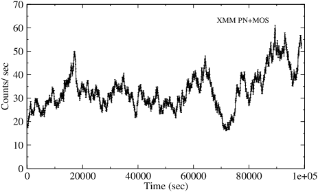
Figure 1: XMM-Newton combined PN and MOS, 0.2–10 keV light curve, binned at 96 s.

2.2 ASCA

We used data taken by ASCA during its long observation of Ark 564, between 2000 June 1 and July 5. The data was reduced as detailed in Papadakis et al. (2002) and we constructed light curves in the 0.7–2 (soft), 2–5 (medium) and 5–10 keV (hard) energy bands for all four detectors, SIS0, SIS1, GIS2 and GIS3. As these data contain regular gaps, due to the Earth occultation of the satellite, we binned the data in orbit-long bins ($\sim 5400$ s) to obtain an evenly sampled light curve, containing 551 points. To check the stability of the detector through this month-long observation, we compared the ratios between the light curves from different detectors. While SIS0, GIS2 and GIS3 showed consistent light curves, we observed discrepancies between these and SIS1 in all energy bands. The ratio between the SIS1 light curve and the light curves from all other detectors shows a linearly decreasing trend, of amplitude $\sim 10$% as measured from the start to the end of the observation. We therefore combined only SIS0, GIS2 and GIS3 data, in each energy band, to produce the final light curves.

The combined, binned and background-subtracted $0.7--10$ keV light curve is shown in Fig. 2. The average count rates for the soft, medium and hard light curves are 2.7, 0.82 and 0.24 counts/s respectively and the average exposure fraction is 23%. The PSD and other variability properties of this data set have been studied by e.g. Papadakis et al. (2002); Edelson et al. (2002).

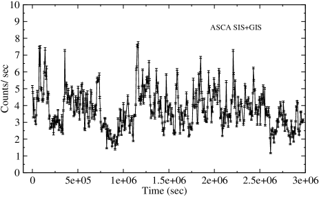
Figure 2: ASCA light curve of Ark 564 in the 0.7–10 keV band, combined data from SIS0, GIS2 and GIS3. The light curve has been binned at 5408 s, which is approximately the orbital period of the satellite.

3 Broad band coherence and lags

Fluxes in different energy bands may vary in a similar way and can do it simultaneously, or with a delay. This relative behaviour can be studied by cross correlating two light curves, observed simultaneously in different energy bands. The cross correlation measures the the degree of linear correlation between the energy bands: if this function presents a significant peak (reaching a value of 1) then the light curves are well correlated and average delay between fluctuations in both light curves is given by the position of this peak on the lag axis. The degree of correlation and the length of the lag might be different for different variability time-scales, therefore it is more convenient to calculate the cross spectrum, which calculates the coherence and time lag for each separate time-scale. This technique uses the Fourier transform of the light curves to separate the different Fourier components at the individual frequencies, and measures the relative phases between the Fourier components of the different light curves. If the relative phases at a given Fourier frequency remain constant between different time segments of the light curves, then the light curves are coherent at this frequency, producing a coherence value of 1. On the other hand, if the phases vary randomly between time segments, the coherence will tend to 0. If the light curves are coherent, their relative phase, i.e. phase lag, represents the delay between similar fluctuations in both energy bands, which can be directly converted into a time lag see section 3 of (see section 3 of Nowak et al., 1999, for an in depth discussion on the meaning of coherence and time lag functions) .

Time lags and coherence between two simultaneous time series $s(t),h(t)$ can be estimated using the cross spectrum $C(f)=S^{*}(f)H(f)$, where $S(f)$ and $H(f)$ are the Fourier transforms of the respective light curves. The coherence $\gamma^{2}$ for discretely sampled time series is calculated as follows:

$$\gamma^{2}(f_{i})=\frac{\langle{\rm Re}_{C}(f_{i})\rangle^{2}+\langle{\rm Im}_{C}(f_{i})\rangle^{2}}{\langle|{\rm S}(f_{i})|^{2}\rangle\langle|{\rm H}(f_{i})|^{2}\rangle},$$ (1)

where ${\rm Re}_{C}(f_{i})$ and ${\rm Im}_{C}(f_{i})$ are the real and imaginary parts of the cross spectrum $C(f)$ and angle brackets represent averaging over independent measurements, either at consecutive frequencies in a frequency bin or equal frequencies from different light curve segments.

The argument of the cross spectrum defines the phase lags: $\phi(f_{i})=\arg{\langle C(f_{i})\rangle}$, and from here the time lags, $\tau(f_{i})$, are calculated as:

$$\tau(f_{i})=\frac{\phi(f_{i})}{2\pi f_{i}}=\frac{1}{2\pi f_{i}}\arctan\left\{\frac{\langle{\rm Im}_{C}(f_{i})\rangle}{\langle{\rm Re}_{C}(f_{i})\rangle}\right\}$$ (2)

The cross spectrum produces estimates of the coherence and time lags as a function of Fourier frequency, or equivalently, of time-scale. Vaughan & Nowak (1997) and Nowak et al. (1999) discuss the interpretation of these measurements in detail and provide error estimates for data with observational noise. We used the methods described therein to estimate the error bars on the time lags.

3.1 Coherence

We used ASCA data to compute lags and coherence in the $10^{-6}-10^{-4}$ Hz frequency range and XMM-Newton data for the $10^{-4}-10^{-2}$ Hz frequency range. Although the data sets were taken 5 years apart, they can be combined as AGN are not expected to change ‘state’ on time-scales of less than $\sim$ 1000 years, assuming linear scaling of the time-scales seen in BHXRBs by the respective black hole masses. This assumption is supported by the fact that the PSD does not change between the observations, at least in the frequency region where the observations overlap (McHardy et al. in prep.) and, as will be shown, the cross spectrum properties also show continuity from one data set to the other.

As a first step we used the $0.7-2.0$ keV and $2.0-10.0$ keV ASCA bands to obtain the highest possible signal-to-noise in the light curves. As the lags and coherence are often energy-dependent, we used XMM-Newton light curves with the same average energies as the ASCA bands (see Section 2.1).

We calculated the cross spectrum for each pair of light curves and binned the coherence and phase lag estimates in logarithmically spaced frequency bins, including a minimum of 10 points per bin. The resulting coherence function is shown by the markers in Fig. 3, where diamonds denote ASCA data points and triangles denote XMM-Newton points. The coherence measurements in this plot have been corrected for Poisson noise effects in the high signal-to-noise limit given by Vaughan & Nowak (1997). The solid and dotted lines represent the scatter expected for each data set, estimated under the assumptions that will be explained in Sec. 3.3. The measured coherence is high ($\sim 0.9$) for the entire frequency range up to $\sim 10^{-3}$Hz. At higher frequencies, the coherence drops drastically (the highest-frequency point is negative, not shown in the plot) but the expected scatter increases significantly, making coherence measurements in this range unreliable.

Figure 3: Coherence between 0.7–2 and 2–10 keV ASCA energy bands and matching XMM-Newton bands, as a function of Fourier frequency. ASCA and XMM-Newton lag estimates are plotted in diamonds and triangles, respectively. The solid line represents the median of the distribution of coherence values from simulated data, as described in Sec. 3.3, the dotted lines represent the top and bottom 95% extremes of this distribution. The simulated light curves have intrinsic coherence of unity. The measured coherence follows the behaviour of the median of the distribution of simulated data, indicating that the drops at the highest frequencies for each data set are (partly) due to noise limitations.

3.2 Time lags

Figure 4 shows the lag spectrum over the frequency range where the measured coherence is high, i.e. below $\sim 2\times 10^{-3}$ Hz, as lags measured in cases of low coherence are not meaningful. Positive lag values indicate that the soft band leads the hard. Significant lags are detected between $\sim 10^{-5}-10^{-3}$ Hz. The XMM-Newton and ASCA lag spectra match well at the frequencies where they overlap, around $10^{-4}$ Hz. The lag spectrum appears to be frequency-dependent, where larger time lags are associated with longer time-scale fluctuations, similar to what has been observed in other AGN and BHXRBs (see Sec. 5.1). The lags spectrum in the frequency range between $2\times 10^{-5}$ and $2\times 10^{-4}$ Hz resembles the shape of a power law. However, at lower and higher frequencies, the measured lags decrease noticeably below the extension of a power law fitted to the lag spectrum in this central frequency range.

A single power law fit to the lag spectrum over the whole frequency range shown in Fig. 4, yields a best-fitting model $\tau(f)=0.04f^{-0.9}$, with a $\chi^{2}=62$ for 14 dof (solid line in Fig. 4). This is clearly an unacceptable fit and leaves the best-defined lag measurements well above the fitted curve. Restricting the fitting range to $\sim 10^{-5}-5\times 10^{-4}$ Hz produces a similar power law, $\tau(f)=0.5f^{-0.7}$, with a $\chi^{2}=9.9$ for 5 dof, shown by the dotted line in the same figure. The measured lags above and below this range fall far below the extension of the power law fit, so the lag spectrum resembles a broad hump. A much better fit to the entire frequency range was obtained by using a single-bend power law model. We chose this model to replicate a power law that bends gently from one slope, $\alpha_{L}$, to another, $\alpha_{H}$, around a bend frequency $f_{b}$, given by:

$$\tau(f)=Af^{\alpha_{L}}/(1+(f/f_{b})^{\alpha_{L}-\alpha_{H}}).$$ (3)

The best fitting values for the low frequency and high frequency slopes ($\alpha_{L}$ and $\alpha_{H}$ respectively) are 0 and -4, while the bend is at a frequency of $2\times 10^{-4}$ Hz. This flat time lag spectrum, bending to a very steep high frequency slope model produces a $\chi^{2}=10.9$ for 16 dof.

The significance of the deviations from a simple power law and the goodness of fit of the bending power law model were assessed through the Monte Carlo simulations discussed in the following section.

Figure 4: Lag spectrum of Ark 564 calculated using ASCA data (diamonds) and XMM-Newton data (triangles) between the 0.7–2 and 2–10 keV ASCA energy bands, plotted as a function of Fourier frequency. The best-fitting power law model for the entire frequency range plotted here ($\tau(f)=0.04f^{-0.9}$) is shown by the solid line. The dotted line represents the best-fitting power law fit to the $10^{-5}-5\times 10^{-4}$ Hz frequency range ($\tau(f)=0.5f^{-0.7}$) and the dashed line represents the best fitting bending power law model, with bend frequency of $2\times 10^{-4}$ Hz and low and high frequency slopes of 0 and -4 respectively. The error bars were calculated following the procedure described by Nowak et al. (1999).

3.3 Estimation of the significance

A power law lag spectrum could be distorted by sampling and observational noise effects. We used Monte Carlo simulations to test the possibilities that the measured lag spectrum deviates from a power law only by these effects and that the drops observed in the coherence function are caused by observational limitations on intrinsically coherent light curves.

We constructed 2000 light curve pairs to simulate simultaneous hard and soft light curves, using the method of Timmer & König (1995). We used a double-bending power law model for the underlying PSD, with the parameters found by McHardy et al. (in prep.):

$$P(f)=Af^{-\alpha_{L}}\left[1+\left(\frac{f}{f_{bL}}\right)^{\alpha_{M}-\alpha_{L}}\right]^{-1}\left[1+\left(\frac{f}{f_{bH}}\right)^{\alpha_{H}-\alpha_{M}}\right]^{-1}$$ (4)

where $A=3\times 10^{4},\alpha_{L}=0,\alpha_{M}=1.2,\alpha_{H}=4.5,f_{bL}=8.7\times 10^{-7}$ Hz and $f_{bH}=2\times 10^{-3}$ Hz. By construction, the light curve pairs have a coherence of unity at all frequencies. Time-scale dependent lags were introduce by shifting the phase component of the Fourier transform of the ‘hard’ simulated light curves, by $2\pi f\tau(f)$. Appropriate Poisson noise was added to the resulting simulated light curves.

ASCA data simulations were generated in 100 s bins and sampled in exactly the same way as the real 100 s binned light curve. They were subsequently re-binned in 5400 s evenly spaced bins, just as was done for the real data. Unlike ASCA data, the real XMM-Newton light curves are practically continuously sampled. Therefore, XMM-Newton simulated light curves were simply generated in 24 s bins and then re-binned in 96 s bins.

The cross spectrum for each pair of simulated light curves was computed using the same binning used for the real data. The median of the distributions of coherence and lag values of the simulations, for each Fourier frequency, are plotted in solid lines in Figs. 3 and 5. The dotted lines in the same figures mark the spread of the distribution of simulated values so that 5% of the points lie above the top line and 5% lie below the bottom line.

The measured coherence in Fig. 3 follows the trend of the median of the distribution of simulations, for both data sets. The small coherence drop on the highest ASCA frequency bins is probably partly due to inaccurate Poisson noise corrections, as suggested by the simulations (the formula for this correction derived by Vaughan & Nowak (1997) is not strictly applicable when the variability signal-to-noise is low). Above this frequency, the coherence drops slightly below the distribution of simulated data, indicating a real but small ($<$10%) loss of coherence. Finally, our results suggest that the strong drop above $10^{-3}$ Hz can be easily explained by Poisson noise effects, and hence is most probably not intrinsic.

As for the phase shift in the Fourier components of the two light curves, initially we used $\tau(f)=0.04f^{-0.9}$, i.e. the best fit to the lag spectrum over the entire frequency range, as the underlying lag spectrum. As seen in Fig. 4 this assumed lag spectrum falls well below the best-defined lag measurements in the middle of the frequency range probed. Not surprisingly, the four central data points remain above the top 95% of the distribution of simulated lags, while two high-frequency points still fall below it, implying that the underlying lag spectrum is inconsistent with the simple power law fitted to the data. We repeated the test using $\tau(f)=0.5f^{-0.7}$ as the underlying lag spectrum, i.e. the fit to the $\sim 10^{-5}-5\times 10^{-4}$ Hz frequency range. The resulting lag spectra distribution is plotted in Fig. 5. The drop in the lags at low and high frequencies is significant as the lags at the extreme frequencies fall far below the 95% lower limit of the distribution of simulated data. We note, also, that the artificial high-frequency break in the lag spectrum, produced by sampling effects and noticed by Crary et al. (1998) cannot explain the break we observe. The artificial break should appear around $0.5\times f_{\rm N}$ where $f_{\rm N}$ is the Nyquist frequency while, for the XMM-Newton data we used, $0.5\times f_{\rm N}\sim 2.6\times 10^{-3}$ Hz, and the break we observe in Ark 564 is at an order of magnitude lower frequency, at $\sim 2\times 10^{-4}$ Hz.

At the low frequency end, the median of the distribution of simulated lag spectra does not reproduce the decreasing trend seen in the data and many data points fall below the 95% lower limit. The small scatter expected in the lag measurements is partly due to the large lags intrinsic to the underlying model we assumed. We repeated the same test, this time using the bending power law as the underlying lag spectrum. The small lags at low frequencies, that this model produces, increases the low frequency scatter significantly. Thereore, a single bend at high frequencies can account for both bends, including the negative lag values of the data at the lowest frequencies. Therefore, a single-bend model, with constant time lags below $\sim 10^{-4}$ Hz is consistent with the data. The median and 95% extremes of the distribution of lag values for the bending power law model are shown in the bottom panel of Fig. 5.

For completeness, we calculated lag spectra using data from the long monitoring campaign of Ark 564 performed with RXTE, described by Pounds et al. (e.g. 2001). The lag spectra obtained from these RXTE data are inconclusive however, as the low variability power below $\sim 10^{-6}$ Hz produces a very weak signal in this frequency range, making lag measurements too uncertain.

We conclude that the changes in slope of the lag spectrum at $\sim 2\times 10^{-5}$ and $\sim 2\times 10^{-4}$ Hz are significant, so the spectrum is not consistent with a single power law model. The spectrum is consistent with a bending power law but we cannot assess accurately the behaviour of the lags below the bend frequency. A model of constant lag up to $10^{-4}$ Hz bending to a $f^{-4}$ dependence at high frequencies can reproduce the data well.

Figure 5: Top: Distribution of simulated lag spectra, using $\tau(f)=0.5f^{-0.7}$ as the underlying lag model, as described in Sec. 3.3. The solid line represents the median and the dotted lines the 95% extremes of the distribution of simulated data. Lags of Ark 564 calculated between 0.7–2 and 2–10 keV ASCA energy bands and matching XMM-Newton bands are plotted in diamonds (ASCA data) and triangles (XMM-Newton data). Filled symbols denote negative lags of the amplitude shown. Below $2\times 10^{-5}$ Hz and above $\sim 3\times 10^{-4}$ Hz, the measured lags fall below the the 5% lowest simulated lag values, indicating that there is a real break in the lag spectrum. Bottom: Same as above but using a bending power law model as the underlying lag spectrum.

4 Energy dependence of the lags

The magnitude of the time lags between energy bands tends to increase with energy separation, in both AGN and BHXRB (e.g. Papadakis, Nandra & Kazanas, 2001; Nowak et al., 1999). In Ark 564, this effect is clearly observable over the frequency range where significant lags can be measured. Figure 6 shows the lags between soft and medium and soft and hard ASCA bands, together with the corresponding XMM-Newton bands. An increase of the energy separation in the bands used to make the cross-spectrum, from a factor 3 to a factor of 6 difference in average energies, produces an increase in the lags by a factor of $\sim 2$, while preserving the shape of the lag spectra, within the uncertainties.

To investigate the energy dependence in more detail, we used the broader energy bandpass of XMM-Newton to construct light curves in 5 different bands, 0.2–0.5, 0.5–1, 1–2, 2–5 and 5–10 keV. The time lags between the 0.2–0.5 keV soft light curve and all the harder light curves are shown in Fig. 7. Here the lags are plotted as a function of the average-energy ratio between each hard band and the 0.2–0.5 band ($E_{H}/E_{S}$), for the three lowest Fourier frequency bins, which had the smallest error bars. In all cases, the lags increase linearly with the logarithm of the energy. The best-fitting relations, plotted in solid lines in Fig. 7, have functional forms: $\tau(E)=1233\log E_{H}/E_{S}-196$ for $7.4\times 10^{-5}$ Hz, $\tau(E)=735\log E_{H}/E_{S}-125$ for $2.0\times 10^{-4}$ Hz and $\tau(E)=199\log E_{H}/E_{S}-38$ for $3.2\times 10^{-4}$ Hz. The errors in the lag values take into account the red-noise nature of the light curves and probably overestimates the relative error between different energy bands. Therefore, the $\chi^{2}$ values for the fits are not significant. A perfect log-linear relation between lag amplitude and energy ratio should cross (1,0) in this plot, as the lags should tend to 0 when calculated between identical energy bands. Therefore, the log-linear relation might not hold down to small energy differences. This possible change in the energy dependence is not significant however, given that if we force the intercepts to equal 0, the fits are still acceptable.

A similar linear dependence of the lags on the logarithm of the energy ratio has been observed for the BHXRB Cyg X-1 (Cui et al., 1997; Crary et al., 1998; Nowak et al., 1999), suggesting that a similar mechanism operates in both sources to produce the time lags.

Figure 6: Time lags between 0.7–2 keV and 2–5 keV (filled diamonds) and 5–10 keV (open diamonds) ASCA light curves. Lags between the corresponding EPIC bands are plotted in filled and open triangles. The lag spectra retain their shape but the amplitude of the lags increase by a factor of $\sim 2$ for a factor of 3 increase in the energy separation of the bands. For clarity, open symbols have been shifted to slightly higher frequencies, their true frequencies being identical to the ones shown by the filled symbols.

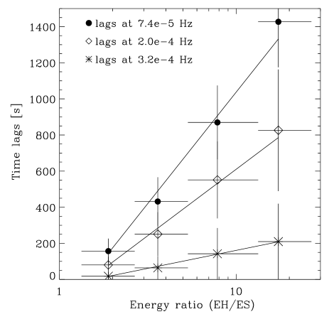
Figure 7: Time lags estimated using the XMM-Newton light curves, between the 0.2–0.5 keV band and the 0.5–1, 1–2, 2–5 and 5–10 keV hard bands, at three temporal frequencies, $7.4\times 10^{-5}$ , $2\times 10^{-4}$ and $3.2\times 10^{-4}$ Hz. The markers are set at the average-energy ratios of the photons in each band, the horizontal lines mark the width of each energy band ratio and are not error bars. The error bars on the lag values were calculated with the prescription of Nowak et al. (1999), notice that this might be an overestimate of the relative error between different energy bands of simultaneous light curves. The lags increase linearly with the logarithm of the energy separation.

5 Discussion

The soft (0.7-2 keV) and hard (2-10 keV) X-ray light curves measured for Ark 564 show highly coherent variability, at least over time-scales of $10^{-6}-10^{-3}$ Hz. These energy bands are dominated by two distinct energy-spectral components, a soft excess dominating up to $\sim 2$ keV and a hard power law dominating at higher frequencies (Turner et al., 2001). These authors have shown, by time-resolved spectral fittings, that these components vary in a similar fashion, albeit with different amplitudes, down to time-scales of at least a day. Given that both spectral components vary, our results of high coherence confirm that the soft excess and the power law variability are well correlated and show that the correlation holds down to time-scales of 1000 s.

5.1 Comparison with other AGN lag spectra

Significant time lags between X-ray energy bands have been measured for a few AGN, NGC 7469 (Papadakis, Nandra & Kazanas, 2001), MCG–6-30-15 (Vaughan et al., 2003), NGC 4051 (McHardy et al., 2004) and NGC 3783 (Markowitz, 2005). In all cases, the lags appear to increase with variability time-scale and, where it has been possible to measure, also with energy separation of the bands. Previous lag spectra were normally fitted with single power law models and, in many cases, only the amplitude of the lags could be left as a free parameter, due to the quality of the data. Consequently, even if there were intrinsic slope changes in the lag spectra of any other AGN, they would not have been detected.

To allow a direct comparison of the amplitude of the lags in different objects, we calculated lag spectra for NGC4051, MCG–6-30-15 and NGC3783 using archival XMM-Newton data in the same PN energy bands as used for Ark 564, i.e. 0.9–2 and 2-4.5 keV. We used these energy bands to plot our Ark 564 XMM-Newton lag spectra together with the ASCA data, matching the average energies of the bands. These AGN lag spectra are shown in the top panel of Fig. 8. The plotted lags are smaller than those published for these objects by other authors because we used closer energy bands and the lags tend to increase with the separation of the energy bands. We plotted fractional lags, given by time-lag/time-scale (equal to $\phi(f)/2\pi$), versus frequency in terms of the PSD break frequency for each object. The PSD break frequency estimates that we used are listed in Table 1 and were taken from literature (references are listed in the same Table). Notice that a constant time lag translates into increasing phase or fractional lags.

The lags in Ark 564, plotted in filled circles in Fig. 8, reach noticeably larger values than all the other objects. Compared to NGC4051 (open diamonds), the shapes and amplitudes are similar in the region where they overlap. At higher relative frequencies, MCG–6-30-15 (filled triangles) and NGC3783 (stars), show much smaller lags. These two objects do show noticeable lags for larger separation of the energy bands, but for the same bands used for Ark 564 their lags are too small to be detected clearly and their spectra are consistent with 0 within the errors. It is possible that in all the objects plotted, the size of the lags drops towards the break frequency in the PSD. If this is the case, the large lags detected in Ark 564 effectively probe a different part of the lag spectrum and we would need lag measurements at lower frequencies in the other AGN to make a significant comparison.

5.2 Comparison with BHXRBs

Figure 8 also shows a comparison of the Ark 564 lag spectrum with the lag spectra of Cyg X-1 in the low/hard and intermediate states. In the low/hard state, plotted in diamonds, Cyg X-1 shows significant fractional lags over more than two decades in frequency. These data correspond to an RXTE long-look observation taken on 1996 Dec 16–19 (total useful exposure time $\sim 89$ ks) and we used $2^{-8}$ s resolution light curves in soft (2–4 keV) and hard (8–13 keV) energy bands. We measured a PSD break frequency at 6 Hz and used this value to scale the lag spectrum shown in Fig. 8. A step-like structure is clearly visible in the low/hard state lag spectrum, which, as noted by Nowak (2000), may be explained if each step corresponds to the lag value of individual broad Lorentzian components in the PSD. A lag spectrum of Cyg X-1 in a transition state is plotted in crosses in the bottom panel of Fig. 8. For this plot we used RXTE data taken on 2000 Nov 3 (ObsID 50119-01-03-01) in the 2–5.7 and 9.4–15 keV energy bands, measuring the PSD break at a frequency of 10 Hz. In this case, the lag spectrum is more clearly ‘peaked’ than in the low/hard state, and the lags are significantly larger (e.g. as noted by Pottschimdt et al. 2000). Lag spectra of a similar peaked shape were found by Miyamoto et al. (1993) in the BHXRB GX 339-4 in the very high state and in the X-ray nova GS1124-68 in the ‘very high flare state’ defined in the same paper.

Although the peaked shape of the Ark 564 lag spectrum resembles slightly one of the steps seen in Cyg X-1 low/hard state, the drops in the case of Ark 564 are much more pronounced and the fractional lag spectrum peak is correspondingly narrower. As Pottschimdt et al. (2000) have shown, the lags in the high/soft and low/hard states of Cyg X-1 are very similar in magnitude and broad time-scale dependence, so the Ark 564 lag spectrum does not correspond to that of a high/soft state either. The strong drops in the lag spectrum of Ark 564, together with the larger amplitude of the lags, show that the data resemble the lag spectrum of Cyg X-1 in the intermediate state (or equivalently, the very high state in BHXRB transients, where similar properties are seen at higher luminosities). Therefore, the spectral-timing data supports the earlier suggestion by Papadakis et al. (2002) that Ark 564 is similar to a BHXRB in the very high state. Although the peak frequencies of the Ark 564 and Cyg X-1 lag spectra are different when scaling by the PSD break frequencies, this difference may reflect the fact that the break-frequencies defined for Cyg X-1 are based on Lorentzian fits to the data, and not the highest-frequency cut-off observed in the PSD, which is probably not detectable due to the low signal to noise at high frequencies in the PSD.

Figure 8: Top panel: Fractional lag (time lag/time-scale) spectrum for Ark 564, in filled circles, compared to lag spectra in the same energy bands of NGC4051 (open diamonds), MCG–6-30-15 (filled triangles) and NGC3783 (stars). The fractional lags are plotted as a function frequency normalised to the PSD high frequency break for each object, as explained in Sec. 5.1. A linear scale was used for the y-axis to allow negative lag points to be plotted. Bottom panel: same as above but comparing with the BHXRB Cyg X-1 in the hard state (diamonds) and one intermediate state (crosses), the PSD break frequencies used were 6 Hz and 10 Hz, respectively.

Object	PSD break	reference
	frequency [Hz]
NGC 3783	$4\times 10^{-6}$	Markowitz et al. 2003
NGC 4051	$8\times 10^{-4}$	McHardy et al. 2004
MCG–6-30-15	$6\times 10^{-5}$	McHardy et al. 2005
Ark 564	$2\times 10^{-3}$	McHardy et al. in prep.

Table 1: PSD break frequencies used for Fig. 8

5.3 Interpretation in terms of variability models

The lag spectrum of Ark 564 shows a constant absolute time-lag over more than a decade range in Fourier frequency, which cuts off at high frequencies, equivalent to a peaked shape in the fractional time-lag spectrum. This shape suggests that only a single variability component, with a single time-lag dominates the variability up until the lag cut-off frequency. It is interesting that the lag cut-off does not correspond to the high-frequency turnover in the PSD, but occurs a decade lower in frequency. This result in turn suggests that a second high-frequency component, with a much smaller (or zero) lag dominates above the lag turnover, and produces the variability observed between $2\times 10^{-4}$ Hz and $2\times 10^{-3}$ Hz. We now consider how this model for the lags can be physically realised.

The X-ray energy spectrum of Ark 564 is composed of a soft excess which dominates below 2 keV and a power law, which dominates at higher energies (Turner et al., 2001). Time lags between soft and hard X-rays could be produced if the soft excess variability leads that of the power law. The energy dependence of the lags, however, indicates that the soft excess cannot lead the power law component as a whole. As shown in Fig. 7, the length of the lags increases with energy separation, so that even energy bands that are fully dominated by the power law component do show different lags. Therefore, the lags must arise at least partly within the power law spectral component.

Several schemes have been proposed to explain the origin of X-ray time lags observed in BHXRBs and AGN. Notably, lags through Comptonisation of seed photons into X-rays of different energies through different numbers of scatterings can produce the observed logarithmic dependence of the lags on energy ratio (see for example discussion in Nowak et al., 1999, section 5.3). In the case of Ark 564 the soft excess photons could serve as input seed photons for a Comptonising corona that would then re-emit them as a power law component, explaining the lag between both components and the increasing lag with energy separation within the power law itself. This simple scheme is challenged by timing considerations, however, given that the larger number of scatterings that the high energy photons must go through reduces their high frequency variability, compared to that of lower energy photons, contrary to what is observed (as noted by e.g. Vaughan et al., 2003). This scenario is also challenged by the frequency dependence of the lags since lags arising simply through Comptonisation would have the same value for all variability time-scales. Therefore, the time lags between the various energy bands most probably arise, at least partly, from the nature of the physical process or by the geometry of the source which is responsible for the hard band power law component. A Comptonisation origin of the lags might still be possible if the Comptonising medium has a radially-dependent electron density, as proposed by Kazanas et al. (1997). Since the turnover in the Ark 564 lag spectrum suggests two separate variability processes with different lags, these might be produced in separate emission regions with different Comptonising structures.

Another possibility is that the lags are produced by accretion rate fluctuations travelling inward through the accretion flow. In this case, the variability fluctuations can be produced quite far out in the accretion flow, so low-frequency variations can still be observed even if most of the X-ray emission originates in the centre of the accretion flow, close to the black hole (Lyubarskii, 1997). If the locally emitted spectrum of the accretion flow hardens towards the centre then the fluctuations are seen first in lower energy bands and later in higher energy bands, which produces the observed hard lags. This scenario was proposed by Kotov et al. (2001) and further discussed by several authors (e.g Vaughan et al., 2003; McHardy et al., 2005; Arévalo & Uttley, 2006) and appears to be consistent with the observed spectral-timing properties of the X-ray light curves, as well as their non-linear nature (Uttley, McHardy & Vaughan, 2005). In particular, the propagating fluctuation model can simultaneously reproduce the high observed coherence, as well as reproducing the lag amplitude and general lag spectral shape and energy dependence of the PSD which is observed in BHXRBs (Arévalo & Uttley, 2006). The required hardening of the energy spectrum towards the centre could be realised by having the soft excess spectral component emitted by an extended region and the power law component produced only close to the centre. A more detailed analysis of the energy spectrum in different variability time-scales would be needed to test this possibility.

In the propagating fluctuation model, a single variability component can dominate the lag spectrum over a broad frequency range if it is produced in a single annulus in the accretion flow, so that the propagation time-scale through the emitting region (and hence the lag) is the same for all variability time-scales. Thus the lag-spectrum of Ark 564 might be produced if the fluctuations arise in two regions in the accretion flow, one, producing variations below $10^{-4}$ Hz at large radii, with detectable lags, and one producing higher-frequency variations at small radii with a negligible lag. If the fluctuation time-scales correspond to the viscous time-scale in a geometrically thick accretion flow, the radii of origin for the low and high-frequency variability components are respectively, of tens of gravitational radii and a few gravitational radii, for the expected black hole mass (Botte et al., 2004) of a few $10^{6}$ M_⊙.

6 Conclusions

We used new XMM-Newton data and combined it with a long ASCA observation to calculate the lags and coherence of Ark 564 over the broadest range of time-scales obtained so far for any AGN. The length of the ASCA observation and the good time resolution of the XMM-Newton data, allowed us to produce an accurate estimate of the coherence and the time lags between different X-ray energy bands.

The coherence was close to unity from $10^{-6}$ down to $\sim 10^{-4}$ Hz. Above this frequency, the coherence drops slightly below the expected scatter inferred from simulations, to a value of $\sim 0.9$. The observed coherence drops by $\sim 10\%$ in the ASCA data, at $\sim 10^{-4}$ Hz and by $30\%$ above $\sim 10^{-3}$ Hz in the XMM-Newton data, i.e. at the shortest time-scales of each data set, are at least partly due to observational biases.

We found significant time lags between different pairs of energy bands, with harder bands lagging softer ones. The magnitude of these hard lags increases with the energy separation of the bands, over the entire frequency range tested. XMM-Newton data was used to show that the amplitude of the lags increases linearly with the logarithm of the energy ratio between the soft and hard bands used, and that the increase is stronger at lower temporal frequencies. The same dependence has been observed before in BHXRBs (e.g Nowak et al., 1999), implying that a similar mechanism operates in both types of source to produce X-ray time lags.

The lag spectrum follows an approximate power law behaviour in the frequency range $10^{-5}-5\times 10^{-4}$ Hz, with a best-fitting slope of $\tau(f)=0.5f^{-0.7}$. Above and below this range, the time lags drop to much lower values. We show that both drops are significant, implying that the lag spectrum is inconsistent with a single power law model, and there is, at least, one change in slope. This broken lag spectrum resembles the lag spectra seen in BHXRBs in the very high or transition state (see e.g. Pottschimdt et al., 2000), and is significantly different to the single power-law lag spectra normally observed in other BHXRB states. Compared with other AGN lag spectra, calculated between the same energy bands, the lags in Ark 564 are larger than all other measurements. The shape and large amplitude of the lags spectrum match well the description of BHXRBs VHS lag spectra as having strongly enhanced lag values over a limited frequency range.

The band-limited lags observed in Ark 564 can be interpreted in terms of a few variability components, perhaps arising from localised annuli in the accretion flow, with a single time lag associated to each of them. If one of these components happens to dominate the variability power over a broad range of time-scales, then its associated lag value would extend throughout the same range. In the case of Ark 564, we note that the two breaks seen in the PSD (Pounds et al. 2001; Papadakis et al. 2002, McHardy et al. in prep.) could correspond to mainly two broad variability components contributing with a large fraction of the total variability power. The lags (of $\sim 600$ s for the ASCA energy bands), seen up to $\sim 10^{-4}$ Hz would correspond to the PSD component peaking at $10^{-6}$ Hz (low frequency PSD break) and a much smaller lag value would be associated with the component peaking at $10^{-3}$ Hz (at the high frequency PSD break). Therefore, the change in slope seen in the lag spectrum can represent the drop from one lag value to the other, or equivalently, the cross-over frequency of the two main variability components.

References

- Arévalo & Uttley (2006) Arévalo P., Uttley P. 2006, MNRAS, 367, 801
- Boller, Brandt, & Fink (1996) Boller T., Brandt W. N., Fink H., 1996, A&A, 305, 53
- Botte et al. (2004) Botte V., Ciroi S., Rafanelli P., Di Mille F., 2004, AJ, 127, 3168
- Crary et al. (1998) Crary D. J., FingerS M. H., Kouveliotou C., van der Hooft F., van der Klis M., Lewin W. H. G., van Paradijs J., 1998, ApJ, 493, 71
- Cui et al. (1997) Cui W., Zhang S. N., Focke W., Swank J. H., 1997, ApJ, 484, 383
- Done & Gierlinski (2005) Done C., Gierlinski M., 2005, MNRAS, 364, 208
- Edelson et al. (2002) Edelson R., Turner T.J., Pounds K., Vaughan S., Markowitz A., Marshall H., Dobbie P., Warwick R., 2002, ApJ, 568, 610
- Kazanas et al. (1997) Kazanas D., Hua X., Titarchuk L., 1997, ApJ, 480, 735
- Kotov et al. (2001) Kotov O., Churazov E., Gilfanov M., 2001, MNRAS, 327, 799
- Lyubarskii (1997) Lyubarskii Y. E., 1997, MNRAS, 292, 679
- Markowitz et al. (2003) Markowitz A., et al. 2003, ApJ, 593, 96
- Markowitz (2005) Markowitz A., 2005 ApJ, 635, 180
- Markowitz & Uttley (2005) Markowitz A., Uttley P., 2005, ApJ, 625, 39
- McClintock & Remillard (2005) McClintock J. E., Remillard R. A., 2005, in Lewin W. H. G., van der Klis M., eds, Compact Stellar X-ray Sources. Cambridge Univ. Press, Cambridge
- McHardy et al. (2004) McHardy I. M., Papadakis I. E., Uttley P., Page M. J., Mason K. O., 2004, MNRAS, 348, 783
- McHardy et al. (2005) McHardy I. M., Gunn K.F., Uttley P., Goad M.R., 2005, MNRAS, 359, 1469
- Miyamoto et al. (1993) Miyamoto S., Iga S., Kitamoto S., Kamado, Y., 1993, ApJ, 403, 39
- Nowak et al. (1999) Nowak M., Vaughan B., Wilms J., Dove J., Begelman M., 1999, ApJ, 510, 874
- Nowak (2000) Nowak, M. A., 2000, MNRAS, 318, 361
- Papadakis, Nandra & Kazanas (2001) Papadakis I. E., Nandra K., Kazanas D., 2001, ApJ, 554,133
- Papadakis et al. (2002) Papadakis I. E., Brinkmann W., Negoro H., Gliozzi M., 2002, A&A, 382, 1
- Merloni, Heinz & di Matteo (2003) Merloni A., Heinz S., di Matteo T., 2003, MNRAS, 345, 1057
- Pottschimdt et al. (2000) Pottschmidt K., Wilms J., Nowak M. A., Heindl W. A., Smith D. M., Staubert R., 2000, A&A, 357, L17
- Pounds et al. (2001) Pounds K., Edelson R., Markowitz A., Vaughan S., 2001 ApJ, 550, 15
- Romano et al. (2004) Romano P., Mathur S., Turner T. J., Kraemer S. B., Crenshaw D. M., Peterson B. M., Pogge R. W., Brandt W. N., George I. M., Horne K., 2004 ApJ,602, 635
- Shemmer et al. (2001) Shemmer O., et al., 2001, ApJ, 561, 162
- Timmer & König (1995) Timmer J., König M., 1995, A&A, 300, 707
- Turner et al. (2001) Turner T. J., Romano P., George I. M., Edelson R., Collier S. J., Mathur S., Peterson B. M., 2001, ApJ, 561, 131
- Uttley & McHardy (2005) Uttley P., McHardy I. M., 2005, MNRAS, 363, 586
- Uttley, McHardy & Vaughan (2005) Uttley P., McHardy I. M., Vaughan S., 2005, MNRAS, 359, 345
- Vaughan & Nowak (1997) Vaughan B., Nowak M., 1997, ApJ, 474, L43
- Vaughan et al. (2003) Vaughan S., Fabian A.C., Nandra K., 2003, MNRAS, 339, 1237