The DEEP2 Galaxy Redshift Survey: Evolution of the Color–Density Relation at $0.4<z<1.35$

Abstract

Using a sample of 19,464 galaxies drawn from the DEEP2 Galaxy Redshift Survey, we study the relationship between galaxy color and environment at $0.4<z<1.35$. We find that the fraction of galaxies on the red sequence depends strongly on local environment out to $z>1$, being larger in regions of greater galaxy density. At all epochs probed, we also find a small population of red, morphologically early–type galaxies residing in regions of low measured overdensity. The observed correlations between the red fraction and local overdensity are highly significant, with the trend at $z>1$ detected at a greater than $5\sigma$ level. Over the entire redshift regime studied, we find that the color–density relation evolves continuously, with red galaxies more strongly favoring overdense regions at low $z$ relative to their red–sequence counterparts at high redshift. At $z\gtrsim 1.3$, the red fraction only weakly correlates with overdensity, implying that any color dependence to the clustering of $\sim L^{*}$ galaxies at that epoch must be small. Our findings add weight to existing evidence that the build–up of galaxies on the red sequence has occurred preferentially in overdense environments (i.e., galaxy groups) at $z\lesssim 1.5$. Furthermore, we identify the epoch $(z\sim 2)$ at which typical $\sim L^{*}$ galaxies began quenching and moved onto the red sequence in significant number. The strength of the observed evolutionary trends at $0<z<1.35$ suggests that the correlations observed locally, such as the morphology–density and color–density relations, are the result of environment–driven mechanisms (i.e., “nurture”) and do not appear to have been imprinted (by “nature”) upon the galaxy population during their epoch of formation.

1. Introduction

The galaxy population both locally and out to $z\sim 1$ is found to be effectively described as a combination of two distinct galaxy types: red, early–type galaxies lacking much star formation and blue, late–type galaxies with active star formation (e.g., Strateva et al., 2001; Baldry et al., 2004; Bell et al., 2004; Menanteau et al., 2006). The spatial distribution of this bimodal galaxy population is frequently phrased today in terms of the so–called morphology–density or color–density relation. As first quantified by Oemler (1974), Davis & Geller (1976), and Dressler (1980), the morphology–density relation holds that star–forming, disk–dominated galaxies tend to reside in regions of lower galaxy density relative to those of red, elliptical galaxies.

Many physical mechanisms that could be responsible for this correlation between galaxy morphology, star–formation history, and environment have been proposed (see Cooper et al., 2006, for a review of probable mechanisms). Are the morphology-density and color–density relations a result of environment–driven evolution, or were these trends imprinted upon the galaxy population during their epoch of formation? Only through comprehensive studies of galaxy properties and environments, both locally and at high redshift, will we be able to understand the role of local density in determining the star–formation histories and morphologies of galaxies.

While the close relationship between galaxy type and density was primarily uncovered via the study of nearby clusters, recent work using the 2–degree Field Galaxy Redshift Survey (2dFGRS, Colless et al., 2001, 2003) and the Sloan Digital Sky Survey (SDSS, York et al., 2000) has established that the connections between local environment and galaxy properties such as morphology, color, and luminosity extend over the full range of densities, from rich clusters to voids (e.g., Kauffmann et al., 2004; Balogh et al., 2004a; Blanton et al., 2005; Croton et al., 2005; Rojas et al., 2005). Furthermore, high–resolution imaging and spectroscopic data in increasingly more distant clusters $({\rm to}\ z\sim 1)$ have shown that the trends observed locally persist to higher $z$, at least in the highest density environments (e.g., Balogh et al., 1997; Treu et al., 2003; Poggianti et al., 2006).

Using a large sample of galaxies drawn from the DEEP2 Galaxy Redshift Survey, Cooper et al. (2006) extended the understanding of the color–density relation at $z\sim 1$ across the full range of environments, from voids to rich groups, showing that the correlation between galaxy color and mean overdensity found locally is in place, at least in a global sense, when the universe was half its present age. While the role of environment appears to have been very critical at $z\sim 1$ and perhaps at earlier times, quantitative measures of the evolution of environmental influences on the galaxy population or of correlations such as the morphology–density and color–density relation are limited.

Comparisons of local results with studies of high–redshift clusters have pointed towards significant evolution in the relationship between galaxy properties and local environment from $z\sim 1$ to $z\sim 0$ (e.g., Dressler et al., 1997; Couch et al., 1998; Smith et al., 2005). While these results indicate an environment–driven evolution in the galaxy population (i.e., pointing towards nurture versus nature as the origin of the galaxy bimodality), such work has been limited to the vicinity of rich clusters, and thus we know little about evolution in the relationship between galaxy type and density across the full scope of galaxy environments. Furthermore, clusters include only a relatively small fraction of the total galaxy population at any epoch by number (and an even smaller fraction by volume). Thus, the evolution of the color–density relation among the vast majority of the galaxy population remains unprobed.

In large clusters, the physical mechanisms at work (e.g., galaxy harassment, ram–pressure stripping, and global tidal interactions) go beyond those acting in group–sized systems and the field. Results from the first comprehensive study of galaxy environment over a broad range of densities at high $z$ indicate that such cluster–specific physical mechanisms cannot explain the global color–density relation as found at $z\sim 1$ (Cooper et al., 2006). Accordingly, in looking for evolution in the relationship between the bimodal nature of galaxy properties and the local galaxy environment, we must turn our attention to the entire dynamic range of galaxy overdensities at high redshift.

In this vein, recent work employing a sample of low– and high–redshift field galaxies from the VIMOS VLT Deep Survey (VVDS, Le Fèvre et al., 2005b) has found a strong evolutionary trend in the color–density relation for galaxies spanning the redshift range $0.25<z<1.5$, with the color–magnitude diagrams for galaxies at $0.9<z<1.5$ showing no significant dependence on environment (Cucciati et al., 2006). Also working at high redshift, a study of the blue fraction (that is, the fraction of galaxies that have blue color) in galaxy groups and in the field population by Gerke et al. (2006) finds instead that the field blue fraction significantly differs from that of the group population out to $z\sim 1.3$.

In this paper, we use the large sample of high–$z$ galaxies obtained by the DEEP2 survey to conduct a detailed study of the color–density relation at $0.4<z<1.35$. In §2, we discuss the data sample employed along with our measurements of galaxy environments and colors. Our main results regarding the relationship between color and environment are presented in §3. Finally, in §4 and §5, we discuss our findings alongside other recent results and summarize our conclusions. Throughout this paper, we assume a flat $\Lambda$CDM cosmology with $\Omega_{m}=0.3$, $\Omega_{\Lambda}=0.7$, $w=-1$, and $h=1$.

2. The Data Sample

2.1. The DEEP2 Galaxy Redshift Survey

The DEEP2 Galaxy Redshift Survey is a nearly completed $(>95\%)$ project designed to study the galaxy population and large–scale structure at $z\sim 1$ (Davis et al., 2003; Faber et al., 2006). To date, the survey has targeted $\sim\!50,000$ galaxies in the redshift range $0.2<z<1.4$, down to a limiting magnitude of $R_{\rm AB}=24.1$. Currently, the survey covers $\sim\!3$ square degrees of sky over four widely separated fields.

In this paper, we utilize a sample of 32,002 galaxies with accurate redshifts (quality ${\rm Q}=3$ or ${\rm Q}=4$ as defined by Faber et al., 2006) in the range $0.4<z<1.35$ and drawn from all four of the DEEP2 survey fields. While at $z>0.75$ the sample includes galaxies from each of the four survey fields, spanning a total of $>\!10$ pointings (Faber et al., 2006), at $0.4<z<0.75$ our sample selection is limited to galaxies in the Extended Groth Strip (EGS), where no color cut to pre–select for $z>0.7$ galaxies was used (Davis et al., 2006).

2.2. Measurements of Rest–frame Colors, Luminosities, and Environments

Rest–frame $(U-B)$ colors and absolute $B$–band magnitudes, $M_{B}$, are calculated from CFHT $B,R,I$ photometry (Coil et al., 2004b) using the K–correction procedure described in Willmer et al. (2006). All magnitudes discussed within this paper are given in AB magnitudes (Oke & Gunn, 1983). For zero–point conversions between AB and Vega magnitudes, refer to Table 1 of Willmer et al. (2006).

For each galaxy in the data set, we compute the projected $3^{\rm rd}$–nearest–neighbor surface density $(\Sigma_{3})$ about the galaxy, where the surface density depends on the projected distance to the $3^{\rm rd}$–nearest–neighbor, $D_{p,3}$, as $\Sigma_{3}=3/(\pi D_{p,3}^{2})$. In computing $\Sigma_{3}$, a velocity window of $\pm 1000\ {\rm km}/{\rm s}$ is utilized to exclude foreground and background galaxies. In the tests of Cooper et al. (2005), this environment estimator proved to be the most robust indicator of local galaxy density for the DEEP2 survey. To correct for the redshift dependence of the sampling rate of the DEEP2 survey, each surface density value is divided by the median $\Sigma_{3}$ of galaxies at that redshift within a window of $\Delta z=0.04$.; correcting the measured surface densities in this manner converts the $\Sigma_{3}$ values into measures of overdensity relative to the median density (given by the notation $1+\delta_{3}$ here) and effectively accounts for redshift variations in the selection rate (Cooper et al., 2005).

Finally, to minimize the effects of edges and holes in the survey geometry, we exclude all galaxies within $1\ h^{-1}$ comoving Mpc of a survey boundary, reducing our sample from 32,002 to 19,464 galaxies. The redshift distribution of this subset is plotted in Figure 1. For complete details regarding the computation of the local environment measures, we direct the reader to Cooper et al. (2006).

Within the DEEP2 sample, the bimodality of galaxy colors in rest–frame $U-B$ color is clearly visible; out to $z\sim 1.4$, the galaxy color–magnitude diagram exhibits a clear division into a relatively tight red sequence and a more diffuse “blue cloud” of galaxies (Willmer et al., 2006). For this study, we compute the fraction of galaxies on the red sequence using the following color division, as defined by Willmer et al. (2006) and illustrated as the dotted lines in Figure 2 and the dashed lines in the lower panels of Figure 3:

$$U-B=-0.032(M_{B}-21.62)+0.454-0.25+0.831.$$ (1)

The red fraction $(f_{\rm R})$ within a given redshift and environment range is given by the number of galaxies redward of this relation in $U-B$ color divided by the total number of galaxies within the same bin of redshift and environment.

As discussed by Willmer et al. (2006), this division between the red sequence and blue cloud is derived from the work of van Dokkum et al. (2000), in which the color–magnitude relation for early–type (i.e., solely morphologically–selected) galaxies is measured. The results of this work and similar studies of clusters at $z<1$ show that ellipticals form a red sequence in color–magnitude space with little scatter (e.g., Ellis et al., 1997; Stanford et al., 1998). Thus, dividing the sample according to the color–cut presented in Equation 1 effectively selects the red, early–type portion of the bimodal galaxy distribution. Details regarding the possible evolution of this color division with redshift are highlighted by Willmer et al. (2006) and examined in §3.1.1 of this work.

Figure 1.— The observed redshift distribution for the 19,464 galaxies in the four surveyed regions which are more than $1\ h^{-1}$ comoving Mpc away from a survey edge and within $0.4<z<1.35$. Galaxies at $z>0.75$ are selected from all four DEEP2 fields, while at $0.4<z<0.75$ galaxies are drawn from the Extended Groth Strip only; in that field, no color–cut is used to pre–select high–redshift ($z>0.7$) sources. In the figure, a dashed line is employed to illustrate this transition in the sample at $z=0.75$. The redshift histogram is plotted using a bin size of $\Delta z=0.025$.

2.3. Sample Selection

Because the DEEP2 survey extends over a broad redshift range, selecting galaxies according to a fixed apparent magnitude limit introduces differences in selection with redshift that depend in a nonnegligible way on galaxy color and luminosity. To study how these selection effects potentially influence our results, we identify several subsamples within the full catalog (Sample A) of 19,464 DEEP2 galaxies spread across the redshift range $0.4<z<1.35$ (cf. Fig. 1). The simplest selection method is to produce a volume–limited subsample according to a strict cut in absolute magnitude. We create such a sample (Sample B) by restricting to $0.4<z<1.1$ and requiring $M_{B}\leq-21$, the absolute magnitude to which DEEP2 is complete along both the red sequence and the blue cloud at $z=1.1$ (cf. top of Figure 2).

Producing a volume–limited sample with a fixed absolute–magnitude limit at all colors severely restricts either the redshift range probed or the number of galaxies selected at each redshift. Here, we adopt a limiting redshift of $z=1.1$ in order to maintain enough galaxies (2,784 in Sample B) with which to accurately compute the red fraction over the full range of overdensities. Given the large redshift range probed in our analysis, however, the number of galaxies with $M_{B}\leq-21$ at low redshift $(0.4<z<0.75)$ is fairly small, and as such results at low $z$ using Sample B are quite noisy.

As discussed by Gerke et al. (2006), in studying the evolution of galaxy properties it is also possible to produce volume–limited catalogs with a color–dependent, absolute–magnitude cut by defining a region of rest-frame color–magnitude space that is uniformly sampled by the survey at all redshifts of interest. For the DEEP2 survey, such a selection cut is illustrated in the bottom of Figure 2 of this paper and Figure 2 of Gerke et al. (2006) and given by

$$M_{\rm{cut}}(z,U-B)=\begin{array}[]{l l}Q(z-z_{\rm lim})+\\ {\rm min}\left\{[a(U-B)+b],\ [c(U-B)+d]\right\},\end{array}$$ (2)

where $z_{\rm{lim}}$ is the limiting redshift beyond which the selected sample becomes incomplete, $a$, $b$, $c$ and $d$ are constants that are determined by the limit of the color–magnitude distribution of the sample with redshift $z<z_{\rm{lim}}$, and $Q$ is a constant that allows for linear redshift evolution of the typical galaxy absolute magnitude $M_{B}^{*}$. For the parameter $Q$, we adopt the Faber et al. (2005) value of $Q=-1.37$, determined from a study of the $B$–band galaxy luminosity function in the COMBO–17 (Wolf et al., 2001), DEEP1 (Vogt et al., 2005), and DEEP2 surveys.

Figure 2.— (Top) The rest–frame color–magnitude diagram for galaxies in the redshift range $1.075<z<1.125$, selected from the full galaxy catalog (Sample A). The dotted vertical line defines the color–independent completeness limit of the DEEP2 survey at this redshift — the absolute–magnitude limit used for Samples B & D. To this limit, the samples are complete for galaxies of all color at $z<1.1$ (Bottom) The rest–frame color–magnitude diagram for galaxies in the redshift range $1.275<z<1.325$, drawn from the full galaxy catalog (Sample A). The dotted line defines the completeness limit of the DEEP2 survey as a function of rest–frame color at redshift $z=1.3$, as given by Equation 2. Due to the $R$–band magnitude limit of the survey, the fraction of red galaxies in the overall DEEP2 sample decreases significantly at high redshift, but by staying within this limit we can construct samples that are free of this effect. The dashed horizontal line shown in both plots illustrates the division between the red sequence and the blue cloud used throughout this paper, following the relation of Willmer et al. (2006) (cf. Equation 1).

By including this linear $M_{B}^{*}$ evolution in our selection cut, we are selecting a similar population of galaxies with respect to $M_{B}^{*}$ at all redshifts. Adopting this approach with a limiting redshift of $z_{\rm lim}=1.3$, we define a sample of 11,192 galaxies (Sample C) over the redshift range $0.4<z<1.3$ that is volume–limited relative to $M_{B}^{*}$ and selected according to this color–dependent cut in $M_{B}$. The values of the constants $a$, $b$, $c$, and $d$ which define the color–dependent selection are $-2.06$, $-18.9$, $-2.63$, and $-18.5$, respectively. For complete details of the selection method, we refer the reader to Gerke et al. (2006).

As a final sample, we again select galaxies assuming linear evolution in $M_{B}^{*}$, as for sample C. However, in determining the limiting absolute magnitude as a function of redshift, we do not apply a color–dependent selection as utilized for Sample C. Instead, we restrict galaxies of all color to the selection limit,

$$\begin{array}[]{c}M_{B}(z)\leq M_{\rm lim}-Q(z_{\rm lim}-z)\\ {\rm or}\\ M_{B}(z)-M_{*}(z)\leq M_{\rm lim}-M_{*}(z_{\rm lim}),\end{array}$$ (3)

where the limiting redshift is chosen to be $z_{\rm lim}=1.1$ and $M_{\rm lim}=-21$ defines the absolute magnitude at $z=1.1$ to which DEEP2 is complete along both the red sequence and the blue cloud (cf. the top panel of Fig. 2). Due to the more severe, color–independent cut in absolute magnitude, Sample D totals only 2,150 galaxies, spanning the redshift range $0.4<z<1.1$. In contrast, while Sample B is similarly selected based just on absolute magnitude (that is, independent of galaxy color), the magnitude cut in Sample D evolves with redshift, staying fixed relative to $M_{B}^{*}$. Thus, Sample B selects galaxies down to the same absolute magnitude at all redshifts, and Sample D samples galaxies to the same depth in the luminosity function at each $z$. A brief summary of the four galaxy samples utilized in this paper is provided in Table 1.

Table 1 Descriptions of Galaxy Samples

Sample	$N_{\rm galaxies}$	$z$ range	Brief Description
Sample A	19,464	$0.4<z<1.35$	all galaxies after boundary cut
Sample B	2,784	$0.4<z<1.1$	color–independent, volume–limited $(M_{B}<-21)$ cut
Sample C	11,192	$0.4<z<1.3$	color–dependent limit, with limit held constant relative to $M_{B}^{*}(z)$
Sample D	2,150	$0.4<z<1.1$	color–independent limit, with limit held constant relative to $M_{B}^{*}(z)$ and set as $M_{B}=-21$ at $z=1.1$

Note. — We list each galaxy sample employed in the analysis, detailing the selection cut used to define the sample as well as the number of galaxies $(N_{\rm galaxies})$ included and the redshift range covered by each sample.

2.4. Mock DEEP2 Survey Catalogs

In order to test for possible systematic effects we employ a set of 12 mock galaxy catalogs based on those of Yan et al. (2004). These catalogs are derived from $N$–body simulations by populating dark matter halos with galaxies according to a halo occupation distribution (HOD) function (Peacock & Smith, 2000; Seljak, 2000), which describes the probability distribution of the number of galaxies in a halo as a function of the host halo mass. The luminosities of galaxies are then assigned according to the conditional luminosity function (CLF) formalism introduced by Yang et al. (2003), which allows the galaxy luminosity function to be mass–dependent as well. Parameters for the HOD and the CLF are chosen to match the 2dFGRS luminosity function (Madgwick et al., 2002) and two–point correlation function (Madwgick et al., 2003). By assuming that the manner in which dark matter halos are populated with galaxies does not evolve from $z\sim 1$ to $z\sim 0$ (Yan et al., 2003) save via an overall evolution in $M_{B}^{*}$ (corresponding to $Q=-1$ here), mock catalogs can then be built using dark–matter–only simulation outputs at varying redshifts. The resulting simulated galaxy catalogs from Yan et al. (2004) are in excellent agreement with the lower redshift $(0.7<z<0.9)$ DEEP2 correlation function (Coil et al., 2004b) and the COMBO–17 luminosity function (Wolf et al., 2003).

It is critical for this paper that we characterize any systematic effects which alter the relationship between galaxy color and observed overdensity as a function of redshift. Therefore, we employ a modified version of the Yan et al. (2004) mock catalogs which incorporate galaxy colors; these catalogs are described in detail by Gerke et al. (2006).

To construct these new catalogs, we first measure the local overdensity of each object in the Yan et al. (2004) mock catalogs using the full, volume–limited catalog. Each galaxy is assigned a rest–frame $U-B$ color drawn from the set of real DEEP2 galaxies at $0.8<z<1.0$ located in a corresponding bin of local galaxy overdensity and absolute $B$–band magnitude, employing the environment measurements of Cooper et al. (2006). This produces mock catalogs which reproduce the observed relationships between galaxy color, luminosity, and environment in the DEEP2 data at $0.8<z<1.0$, but do not allow those relationships to evolve with redshift unless the “true” distribution of galaxy overdensities evolves. After galaxy colors are assigned, apparent $R$ magnitudes are determined using the K–correction methods applied for DEEP2 (Willmer et al., 2006), so that red galaxies will be lost at the same luminosity at a given redshift as in the data. We then apply the standard DEEP2 target–selection and slitmask–making procedures (Davis et al., 2003; Faber et al., 2006) to these mock catalogs, so that we may directly determine the effects of DEEP2 target–selection algorithms on observed trends.

These mock catalogs should not be a perfect representation of reality, as uncertainties in the observed environments will cause some objects to be assigned the color of a galaxy that is actually in a higher– or lower–density environment than was measured; however, this effect is small (i.e., environment measurement errors at $z=0.8-1$ are significantly smaller than the bin sizes). Nevertheless, they provide a robust test of whether we may falsely observe an evolution in the relationship between galaxy color and environment when in fact none exists. They also allow us to directly explore what effects the increased errors in environment measurements at higher redshifts (where samples grow dilute) may have on our results. We discuss these tests in §3.2.

3. Results

3.1. The Color–Density Relation at $0.4<z<1.35$

Figure 3 shows the relationship between the red fraction $(f_{\rm R})$ and local galaxy overdensity for the full data set (Sample A) in four distinct redshift bins spanning $0.4<z<1.35$. We find that the red fraction exhibits a strong dependence on local environment in each redshift bin, such that $f_{\rm R}$ is higher in regions of greater overdensity. Fitting a linear relation to the trends in Figure 3, we find that the slope of this color–environment correlation evolves with $z$, with the relative fraction of red galaxies in dense environments decreasing with lookback time (cf. Table 2). Over the full redshift range probed by the DEEP2 sample, the measured slope decreases from ${\rm d}f_{\rm R}/{\rm d}\log_{10}(1+\delta_{3})=0.111$ for $0.4<z<0.75$ to ${\rm d}f_{\rm R}/{\rm d}\log_{10}(1+\delta_{3})=0.046$ for $1.0<z<1.35$, with the difference being significant at a greater than $3$–$\sigma$ level.

The vertical error bars in Figure 3 indicate the Poissonian uncertainty in each point. Error estimates based on bootstrap and jackknife resampling amongst the 10 DEEP2 pointings used yielded comparable uncertainties (within 10–20%), suggesting that sample (or “cosmic”) variance is not the dominant source of uncertainty; while cosmic variance will influence the distribution of environments in a given redshift bin, it should not strongly affect the relationship between galaxy color and density in a given environment bin. Refer to §4.1 for further investigation of the role of cosmic variance in this analysis.

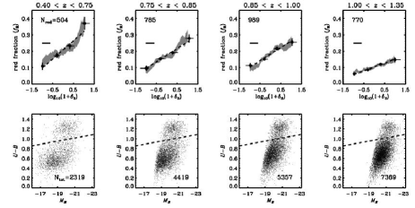
Figure 3.— Top Row: Using the full galaxy sample (Sample A), we plot the red fraction as a function of overdensity, $\log_{10}(1+\delta_{3})$, in four distinct redshift ranges (redshift limits indicated at the top of each column). The circular points give the red fraction as function of the median overdensity, computed in four distinct bins of $\log_{10}(1+\delta_{3})$. The horizontal error bars run from the twenty–fifth percentile to the seventy–fifth percentile of the overdensity distribution in each bin. The vertical error bars give the 1–$\sigma$ uncertainty on the red fraction within each overdensity bin, given by Poisson statistics. The grey shaded region in each panel shows the 1–$\sigma$ range of the red fraction as a function of median overdensity in a sliding bin with width given by the horizontal line segment in the upper left of each plot $(\Delta\log_{10}{(1+\delta_{3})}=0.2)$. The number in the upper left corner denotes the total number of red galaxies in the particular redshift interval. The dashed line in each panel shows a linear–regression fit to the four data points, with coefficients given in Table 2. Bottom Row: We plot the rest–frame color–magnitude relation for all objects in each redshift bin. The division between the red sequence and the blue cloud is given by the dashed line, following the relation of Willmer et al. (2006) (cf. Equation 1). The total number of galaxies (both blue and red) in each $z$ bin is enumerated in the bottom right corner and given in Table 2.

All of the samples described in §2.3 yield similar results for the evolution of the color–density relation (cf. Fig. 4 and Table 2). While overall $f_{\rm R}$ values by overdensity differ when either a color–dependent or a color–independent $M_{B}$ limit is applied to the full sample, in every case the color-environment relation weakens, but still is present, at higher $z$. Due to their small sample sizes, the effect is not statistically sigificant for Samples B and D, however.

Table 2 Linear Fits to the $f_{\rm R}$-overdensity Relation

	$N_{\rm red}$	$N_{\rm tot}$	$a_{0}$ (slope)	$a_{1}$ ($y$–intercept)	$\sigma_{\rm slope}$	$\sigma_{y{\rm-int}}$
Sample A
$0.4<z<0.75$	504	2319	0.111	0.208	0.018	0.010
$0.75<z<0.85$	785	4419	0.081	0.175	0.012	0.007
$0.85<z<1.0$	989	5357	0.080	0.182	0.012	0.006
$1.0<z<1.35$	770	7369	0.047	0.104	0.007	0.004
Sample B
$0.4<z<0.75$	48	76	0.240	0.546	0.230	0.140
$0.75<z<0.85$	125	297	0.127	0.395	0.076	0.044
$0.85<z<1.1$	464	1081	0.120	0.413	0.047	0.024
Sample C
$0.4<z<0.75$	116	813	0.103	0.131	0.019	0.013
$0.75<z<0.85$	207	2143	0.066	0.093	0.012	0.007
$0.85<z<1.0$	282	2868	0.056	0.097	0.011	0.006
$1.0<z<1.3$	372	5368	0.035	0.068	0.007	0.004
Sample D
$0.4<z<0.75$	76	148	0.194	0.446	0.098	0.069
$0.75<z<0.85$	102	237	0.150	0.405	0.086	0.049
$0.85<z<1.1$	347	844	0.090	0.403	0.056	0.026

Note. — We list the coefficients and 1–$\sigma$ uncertainties for the parameters of the linear-regression fits to the red fraction versus median overdensity relation given by $f_{\rm R}=a_{0}\cdot\log_{10}(1+\delta_{3})+a_{1}$ (cf. Fig. 3 and Fig. 4) in each $z$ bin employed for all four galaxy samples used. We also give the number of red–sequence members $(N_{\rm red})$ along with the total number of galaxies $(N_{\rm tot})$ in each redshift bin for that sample. For details regarding the various galaxy samples, refer to §2.3 and Table 1.

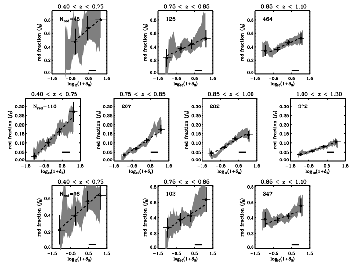
Figure 4.— We plot the red fraction as a function of overdensity, $\log_{10}(1+\delta_{3})$, in distinct redshift ranges for the remaining three galaxy samples identified in §2.3 and summarized in Table 1 — Samples B (Top Row), C (Middle Row), and D (Bottom Row). The circular points give the red fraction as function of the median overdensity, computed in distinct bins of $\log_{10}(1+\delta_{3})$. The horizontal error bars run from the twenty–fifth percentile to the seventy–fifth percentile of the overdensity distribution in each bin. The vertical error bars give the 1–$\sigma$ uncertainty on the red fraction within each overdensity bin, given by Poisson statistics. The grey shaded region in each panel shows the 1–$\sigma$ range of the red fraction as a function of median overdensity in a sliding bin with width given by the horizontal line segment in the lower right of each plot $(\Delta\log_{10}{(1+\delta_{3})}=0.2)$. The number in the upper left corner denotes the total number of red galaxies in the particular redshift interval. The dashed line in each panel shows a linear–regression fit to the data points, with coefficients of the fit given in Table 2. For the each sample, the baseline value of $f_{\rm R}$ varies significantly as the different sample selection criteria include different portions of color–magnitude space.

To further illustrate the evolution in the color–density relation with $z$, we present color–magnitude diagrams in Figure 5 divided by local environment and redshift. In this figure, the relationship between red fraction $(f_{\rm R})$ and galaxy overdensity is made directly discernable to the eye; in high–density regions, there is an increased proportion of sources on the red sequence relative to that observed in low–density environments.

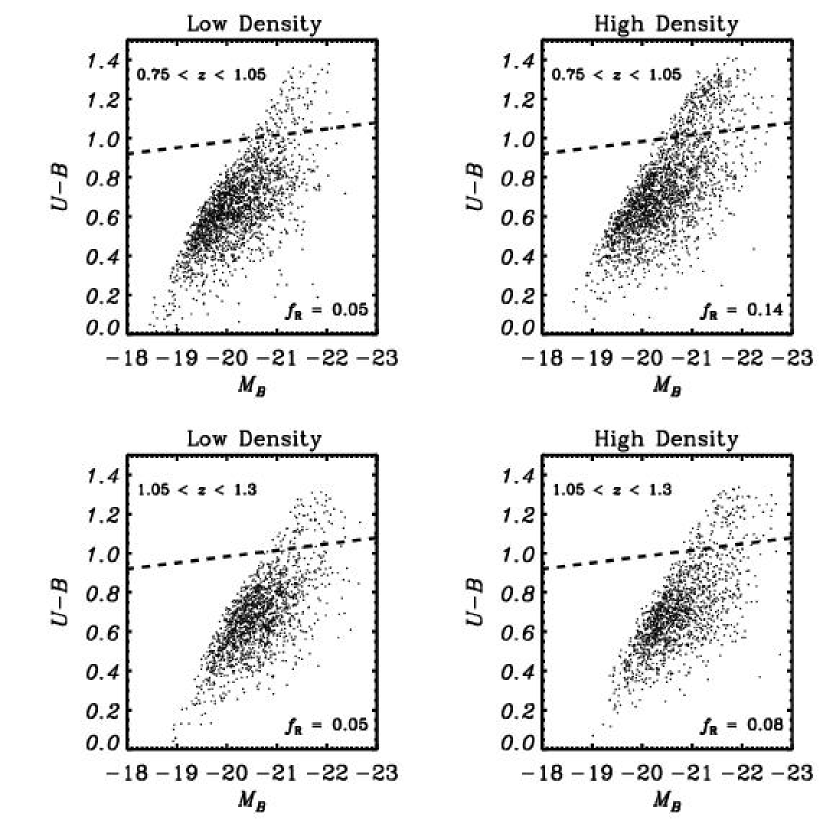
Figure 5.— We plot the color–magnitude relation for DEEP2 galaxies in low–density and high–density environments at low and high redshift. Here we use “low” and “high” density to refer to the extreme thirds of the overall overdensity distribution within Sample C. The dashed line in each plot denotes the division between the red sequence and blue cloud as given in Equation 1. At the bottom right corner of each plot, the red fraction $(f_{\rm R})$ for that color–magnitude diagram is given. For each row, the two panels contain equal numbers of objects. The greater prevalence of red objects in high–density regions, particularly at lower redshifts, is readily apparent to the eye.

While the results shown in Figure 3 show a clear signature of evolution in the color–density relation over the redshift range $0.4<z<1.35$, relatively large redshift bins are used, thereby coarsely sampling the redshift domain. To study the evolution of the $f_{\rm R}$–overdensity relationship with $z$ in more detail, we divide Sample C into thirds according to overdensity and compute the red fraction as a function of redshift in a sliding bin of width $\Delta z=0.1$ for the galaxies in the high–density $(\log_{10}{(1+\delta_{3})}\gtrsim 0.25)$ and low–density $(\log_{10}{(1+\delta_{3})}\lesssim-0.2)$ extremes of the overdensity distribution, with results shown in Figure 6. Here, the high–density and low–density thirds are defined with respect to the overdensity distribution in each $z$ bin; however, dividing the galaxy sample into high– and low–density regimes according to the overdensity distribution in the entire redshift range $(0.75<z<1.3)$ probed yields consistent results. As detailed in §2.3, sample C is defined so as to be complete with respect to $M_{B}^{*}$ across the full redshift range, $0.4<z<1.3$, establishing a sample uniformly selected at all redshifts studied.

As illustrated in Fig. 6, the color–density relation shows a continuous evolution with redshift from $z\sim 0.75$ to $z\sim 1.3$, such that at redshifts approaching $z\sim 1.3$ the red fraction in low– and high–density regions are statistically consistent with each other. Extrapolating linear regression fits to the $f_{\rm R}(z)$ relations in high–density and low–density environments, we find convergence at a redshift of $z=1.32$. We investigate this convergenece in more detail in the following subsections (§3.1.2 and §3.1.3).

In our analyses, we have attempted to carefully account for selection effects due to the design parameters of the DEEP2 survey. For all galaxy samples but Sample A, selection effects related to the survey’s magnitude limit and $R$–band selection, which bias the sample against faint and/or red galaxies at higher redshifts, shoud be minimal. The agreement amongst the highly disparate samples indicates that the results presented above are robust to such effects.

These results are similar to the findings of Gerke et al. (2006), which investigates the evolution of the blue fraction among group and field galaxies at $0.7<z<1.3$ in DEEP2. That work employed a very different technique for measuring galaxy environment and studied a somewhat different set of galaxy subsamples. The measurements of the evolution in the blue fraction presented by Gerke et al. (2006), however, are significantly noisier than those presented in this study and could be susceptible to biases if the group–finding algorithm used performs differently at different $z$. We note that while that work uses a different methodology for dividing galaxies into environment bins (identifying members of galaxy groups rather than with a continuous measure of local galaxy density), both the Gerke et al. (2006) results and those presented here are derived from subsamples of the DEEP2 survey; hence any systematics affecting one may also affect the other.

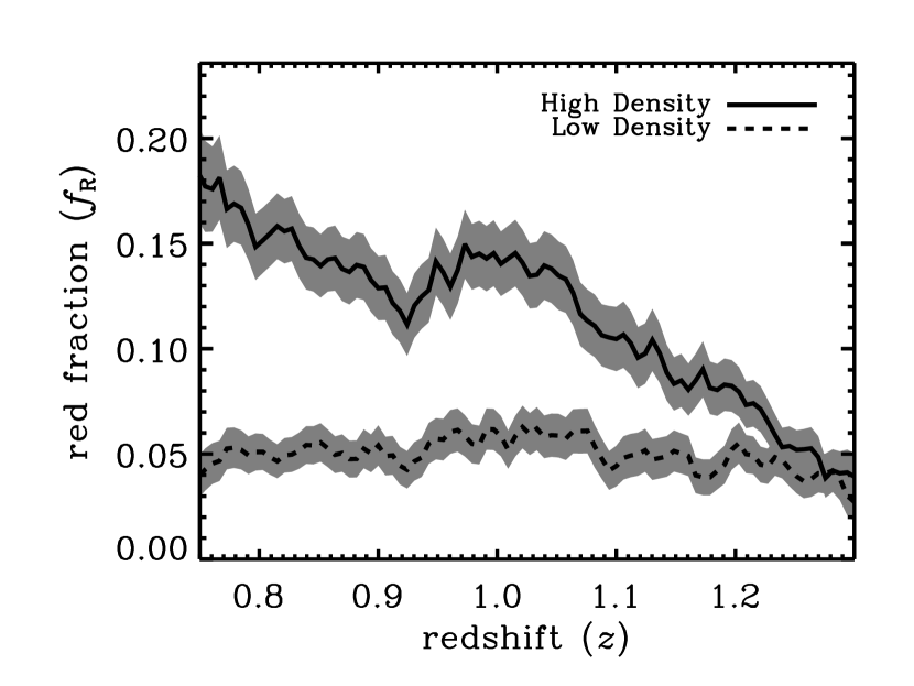
Figure 6.— For galaxies in Sample C within high–density (solid line) and low–density (dashed line) environments, we plot the red fraction $(f_{\rm R})$ as a function of redshift for galaxies in sliding bins of $\Delta z=0.1$. The high– and low–density samples are selected according to the extreme thirds of the local overdensity $(1+\delta_{3})$ distribution in the given $z$ bin. The grey shaded regions give the 1–$\sigma$ range of the red fractions in each density regime. The color–density relation evolves significantly over the redshift range $0.75<z<1.3$, with the red fraction in high–density environments dropping continuously as $z$ increases, while in low–density regions it remains relatively constant at all redshifts probed. At $z\sim 1.3$, the red fraction shows no dependence on environment within the measurement errors.

3.1.1 Effect of Possible Evolution in the Color of the Bimodality

While the position of the bimodality in $U-B$ versus $M_{B}$ color–magnitude space shows no significant dependence on redshift within the DEEP2 data, when studying the red fraction as a function of redshift, we must consider the possibility that there is evolution in the color of the red–sequence population and thus in the position of the color bimodality. If the location of the color bimodality evolves with reshift, then the measured evolution in the red fraction in high–density environments could simply result from galaxies moving (e.g., via passive evolution) across our non–evolving color division (cf. Equation 1). However, any affect related to possible evolution in the location of the $U-B$ bimodality would be minimized by the differential nature of our measurements. That is, the location of the color bimodality does not appear to depend on environment, and thus any evolution in the red fraction for the galaxy sample in high–density regions should be mirrored in the $f_{\rm R}(z)$ for the sample of galaxies in intermediate– and low–density environments.

Furthermore, given that passive evolution will cause galaxies to move redward as they evolve and that the $U-B$ color division in Equation 1 is defined by a galaxy sample at $z\sim 0.8$ (Willmer et al., 2006; van Dokkum & Franx, 2001), a non–evolving color division will not increase the measured evolution in the color–density relation due to an interloper population of blue galaxies on the red sequence at $z>1$. Instead, a non–evolving cut would create a more stringent selection criterion at higher redshifts, limiting the number of galaxies residing in the trough between the red sequence and blue cloud (also called the “green valley”) that are counted as members of the red sequence, thereby actually producing weaker evolution in the color–density relation.

In the spirit of thoroughness, however, we test the effect of using an evolving color division on our results. Allowing for passive evolution in the location of the color bimodality of $\sim 0.15$ magnitudes (in $U-B$) per unit $z$ (e.g., van Dokkum & Franx, 2001; Blanton, 2006), such that the division between red and blue galaxies moves blueward with lookback time, we find no significant change in our results. That is, employing a redshift–dependent division between the blue cloud and red sequence, the relative red fraction in high– and low–density environments still shows strong evolution, consistent with no color–density relation at $z\sim 1.35$.

3.1.2 Effect of Redshift Incompleteness

In analyzing the evolution of the red fraction $(f_{\rm R})$ as a function of redshift, we must consider the possible impact of redshift–dependent selection effects in the DEEP2 survey. In particular, due to the finite amount of slit–length real estate available on DEIMOS slitmasks and the finite amount of observing time dedicated to the project, the DEEP2 survey only spectroscopically observes $\sim\!60\%$ of the galaxies that meet the survey’s target–selection criteria. Furthermore, about $30\%$ of those galaxies targeted for spectroscopy fail to yield a high–quality (quality $Q=3,4$) redshift.

Initial follow–up observations of sources for which DEEP2 fails to measure a redshift indicate that roughly half of all failures (i.e., $\sim\!15\%$ of DEEP2 targets) are at redshifts beyond the range probed by DEEP2 (i.e., $z\gtrsim 1.4$; C. Steidel, private communication). Additionally, redshift failures may result from poor observing conditions, data reductions errors, or instrumental effects. Clearly important for this work is the fact that the DEEP2 redshift failure rate is correlated with observed galaxy color and magnitude, thus possibly introducing bogus trends in the measured $f_{\rm R}(z)$ relation.

To understand the degree to which our results are impacted by redshift incompleteness, we employ the weighting scheme presented by Willmer et al. (2006). The derived weights account for variations in both redshift incompleteness and targeting rate as a function of apparent $R$ magnitude and apparent $R-I$ and $B-R$ colors, assuming that the redshift distribution for red $(R-I>1.03)$ failures is identical to that of the observed (quality $Q=3,4$) red galaxy sample and that the blue $(R-I<1.03)$ failures sit beyond the redshift range of the survey (defined as the “optimal” model in Willmer et al., 2006). If we use these weights to compute $f_{\rm R}(z)$ for Sample C (as in Fig. 6), all changes in the measured trends with redshift are well within the measurement uncertainties. Thus, biases related to redshift incompleteness should not introduce spurious results in our analysis. With and without weighting for incompleteness, we find a convergence of the red fraction in high– and low–density environments at $z\gtrsim 1.3$; extrapolating linear regression fits to the $f_{\rm R}(z)$ relations in high–density and low–density environments, we find convergence at a redshift of $z=1.33$ when weighting for incompleteness versus a convergence at $z=1.32$ without weighting.

3.1.3 Tests with Mock Galaxy Catalogs

The mock galaxy catalogs described in §2.4 allow us to further test the degree to which our observations of the color–density relation may be subject to systematic effects within DEEP2 (e.g., due to increased errors in environment measures as the sampling density drops with $z$ or due to the expected changes in the magnitude of peculiar velocities with $z$ compared to the 1000 ${\rm km}/{\rm s}$ window used). These catalogs should exhibit no evolution in the color–density relation when measured with perfect information, by construction. Therefore, when we apply our measurement techniques to subsets of the mock catalogs which emulate the observed samples, any apparent evolution in the color–density relation will generally indicate the presence of observational biases.

There is a notable exception to this. It is possible to select a subsample from the volume–limited mock galaxy catalog (i.e., the catalog before applying DEEP2 target–selection criteria or slitmask–making algorithms) using a color–dependent, absolute–magnitude limit which evolves with $z$, as for our Sample C above; however, for the mock catalogs, $Q=-1$ is the appropriate evolution, as that value was used in their construction, rather than $Q=-1.37$ as used for Sample C. We find that if we use the full volume–limited mock catalog to determine local overdensities in real–space, there is in fact evolution in the color–density relation for such a sample (cf. Figure 7a).

This evolution does not reflect an observational selection effect, however. Instead, it is a result of applying an absolute–magnitude cut which changes with $z$ to mock catalogs which were constructed assuming rest–frame color depends on $M_{B}$ in a way which is independent of $z$ (cf. §2.4). Because $M_{B}^{*}$ was brighter at higher $z$, the galaxies included by DEEP2 tend to be brighter at higher $z$; and as may be seen in Fig. 2 and Fig. 5, brighter galaxies are more likely to be red. The color–dependent, absolute–magnitude limit exaggerates this effect. If instead we apply a color– and redshift–independent absolute–magnitude limit to the volume–limited mock sample, the mock catalogs show considerably weaker color–density evolution, as we would expect (cf. Fig. 7b). For panels (a) and (b) of Figure 7, we determine the “true” local galaxy environment according to the $7^{\rm th}$–nearest–neighbor surface density (converted into an overdensity, $(1+\delta_{7})$) using the real–space galaxy positions and the full volume–limited galaxy population.

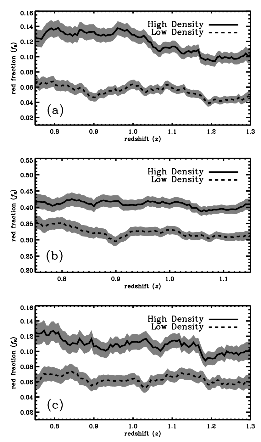
Figure 7.— For the mock galaxy samples, we plot the red fraction $(f_{\rm R})$ as a function of redshift in high–density (solid line) and low–density (dashed line) environments where the high–density and low–density samples are selected as the extreme thirds of the environment distribution for the given galaxy sample. The shaded grey regions in each plot trace the 1–$\sigma$ range of the red fractions in each density regime. Both plots (a) and (b) utilize “true” environment measures defined using the entire volume–limited mock catalog. However, (a) shows $f_{\rm R}(z)$ for a DEEP2–like “observed” sample, while (b) gives the same relation for a sample selected according to a fixed (that is, redshift–independent) $M_{B}<-20$ absolute–magnitude limit. Like (a), panel (c) uses a DEEP2–like “observed” sample. In contrast, though, panel (c) employs environments estimated according to the overdensity $(1+\delta_{3})$ as measured in the “observed” sample (i.e., using redshift–space galaxy positions and the DEEP2–like galaxy sample). The differences between (a) and (c) are consistent with a scenario where noise in environment measures causes the color–density relation at high redshift to be smeared out. However, such observational selection effects cannot alone explain the convergence of $f_{\rm R}$ that we observe at $z\sim 1.3$ in the DEEP2 data (cf. Fig. 6). For more details regarding the specific sample selection criteria and environment measures, refer to the text of §3.1.3.

Although the mock catalogs exhibit a modest evolution in the color–density relation for samples with an absolute–magnitude limit that shifts with $M^{*}$ (like our Sample C), they still may be used to determine the net effects of DEEP2 sample selection on the observed color–density relation. We do this by comparing $f_{\rm R}(z)$ in two different mock catalog samples. For the first, we do not apply DEEP2 target–selection and slitmask–making criteria, but only the color–dependent absolute–magnitude limit given by Equation 2 with $Q=-1$, and we use the best possible measure of environment in the catalogs (based upon the real–space overdensity of galaxies in the full, volume–limited catalog, as employed by Cooper et al., 2005) to divide the sample into environment bins; see Fig. 7a. For the second, we apply the DEEP2 target–selection and slitmask design algorithm to these mock catalogs, and use the overdensity measured from this “observed” sample to partition the sample; results for this sample are shown in Fig. 7c.

We find that in fact the DEEP2–like sample exhibits both a smaller gap between $f_{\rm R}(z)$ for the extreme environment bins and a stronger apparent evolution over $0.75<z<1.3$. This is consistent with a scenario where noise in environment measures causes objects to cross the boundary between the intermediate environment bin and the extremes, thereby artificially increasing the red fraction for the low–density sample while decreasing $f_{\rm R}$ for the high–density sample. This effect should become worse at higher $z$, as the sampling density decreases there, leading to greater environment errors. Therefore, though we observe convergence of between the red fraction in low– and high–density environments at $z=1.32$, in actuality convergence should not occur until a somewhat higher redshift.

However, this test shows that observational selection effects cannot explain the convergence in $f_{\rm R}$ that we observe in high–density and low–density regions at $z\sim 1.3$. Extrapolating linear–regression fits to the $f_{\rm R}(z)$ relations in high–density and low–density environments, we find convergence at $z=2.50$ if we measure environment with the full sample (Fig. 7a), or $z=2.29$ after we apply DEEP2 target selection procedures (Fig. 7c). The mock catalogs provide clear evidence that the null hypothesis of no evolution in the color–magnitude relation over $0.75<z<1.3$ cannot hold.

3.2. Red Galaxies in Low–Density Environments

The relations presented in Figure 3 also show evidence of a trend with $z$ in the normalization of the $f_{\rm R}$–overdensity relation, such that the total fraction of red–sequence galaxies averaged over all densities decreases with $z$. This effect is dominated by two systematic trends in the data: (1) from $z\sim 0$ to $z\sim 1$, the number density of red galaxies in the universe decreases by a factor of $\sim\!2$–3 (e.g., Bell et al., 2004; Faber et al., 2005), and (2) at redshifts beyond $z\sim 1.1$, the red galaxy fraction decreases precipitously in the DEEP2 sample, due to the survey’s $R$–band magnitude limit (Cooper et al., 2006). This latter effect is quite apparent in the final redshift bin in Figure 3, where the normalization of the observed red fraction–overdensity relation drops significantly; the other volume–limited samples studied here should not be affected by this, however (cf. Fig. 4).

In spite of these redshift–dependent effects, we still find that at all redshifts probed in this paper some fraction of red galaxies populate very underdense environments. While uncertainties in the environment measurements will lead to some galaxies at intermediate densities being scattered into the low–density third of the overdensity distribution, upper limits on this effect show that it cannot account for all of the red galaxies found in low–density environments at any redshift, as we now show. We proceed by assuming that the observed $\log_{10}{(1+\delta_{3})}$ distribution of red galaxies matches the shape of the true distribution, an assumption that holds so long as the distribution is approximately linear over scales comparable to measurement errors (as convolving a linear function with a Gaussian leaves it unchanged). In actuality, e.g. if the $\log_{10}{(1+\delta_{3})}$ distribution has some cutoff value at low overdensity, the observed distribution will have more objects below this cutoff than the true distribution; thus the observed distribution provides an upper limit to the true contamination rate.

We calculate this limit from the expectation value of the number of red objects that have true overdensities in the top two–thirds of galaxies but measured overdensities in the lowest one–third, minus the number of objects truly in the bottom one–third but measured in the top two–thirds. We assume that each overdensity measurement may be represented by a Gaussian distribution in $\log_{10}{(1+\delta_{3})}$, with mean given by the measured value and standard deviation increasing linearly from $\sigma=0.49\ {\rm dex}$ at $z=0.8$ to $0.59\ {\rm dex}$ at $z=1.2$, based upon tests with the mock catalogs described in §2.4. We find that the increasing uncertainties in environment measures combined with the weakening in the strength of the color–density relation with lookback time yield a net contamination rate that is roughly constant with redshift $(\sim 35\%)$. Hence, the true red fraction in the extreme low–density third of the sample is at least $3\%$ at all redshifts. Similar studies at lower redshift (e.g., Balogh et al., 2004b; Yee et al., 2005; Croton et al., 2005; Martínez et al., 2006) have shown that the existence of red galaxies in low–density environments persists to $z\sim 0$.

Clearly, a population of red galaxies in low–density environments exists at $0.75<z<1.3$. However, galaxies may appear red either because they are true red–sequence/early–type galaxies or because of the presence of interstellar dust. Based on past studies (e.g., Lotz et al., 2006), we might expect the former population to dominate the red sequence at lower redshift and the latter at higher $z$. Are the red–sequence members in low–density regions at low and high redshift comparable in terms of galaxy morphology? Out of the less than 40 red galaxies in underdense environments identified in DEEP2 for which HST/ACS imaging is available in the EGS (Davis et al., 2006), an initial by–eye inspection indicates that the majority of this population exhibits early–type morphologies, with the remainder being reddened disk galaxies. While the sample imaged with HST/ACS is small, we find no significant trends of morphology with redshift; for example, dusty disk galaxies do not increasingly dominate the red sequence in low–density environments at higher $z$. However, contamination by late–type galaxies preferentially at higher $z$ cannot be excluded as a possible explanation for the observational results presented here; an analysis of galaxy morphologies by Lotz et al. (2006) concludes that late–type galaxies comprise 30% of the red sequence at $z\gtrsim 1$, though they are only a minor contaminant at low redshift (see also Weiner et al., 2005). Such an increase in the contribution of dusty disks to the red sequence at $z>1$ could work to reduce the strength of an existing color–density relation.

Are members of the red sequence in underdense regions the result of passive evolution, in which they consumed their gas supplies independent of environmental effects, or are they fossil groups that result from the merging of several smaller galaxies? Clearly, even in underdense environments galaxy mergers are capable of triggering events that reduce gas reservoirs and at least temporarily halt star formation as well as disrupt galactic disks, yielding merger remnants with surface–brightness profiles and density distributions similar to those of early–type galaxies (Toomre & Toomre, 1972; Navarro et al., 1987; Barnes & Hernquist, 1992; Hopkins et al., 2005). Similarly, passive evolution when teamed with processes attributed to secular evolution such as bar instabilities could also explain the existence of red, morphologically early–type galaxies in low–density environments (Zhang, 1996). In future work, we hope to explore the morphologies of red galaxies in low–density regions within the EGS in more detail, with a goal of differentiating between these two scenarios; galactic bulges formed by bar instabilities tend to differ from those built via mergers in that the former exhibit more disk–like properties such as flatter profiles and residual bars or spiral structure (Kormendy & Fisher, 2005).

4. Discussion

4.1. Comparison with Related Studies

From our study of 19,464 galaxies in the DEEP2 Galaxy Redshift Survey, we conclude that the color–density relation observed in the local universe is also seen at $z>1$, with the fraction of red galaxies increasing with local galaxy overdensity at essentially all epochs studied $(0.4<z<1.35)$ and over all environments probed (from voids to large groups). At all redshifts, however, there still exists a population of red galaxies in underdense environments. In addition, we find that the color–density relation evolves with redshift, growing weaker with lookback time such that at $z\gtrsim 1.3$ the relationship may be nonexistent within the range of environments probed by the DEEP2 survey (i.e., not including massive clusters). When viewed in conjunction with the results from studies of the galaxy luminosity function at $0<z<1$ (Bell et al., 2004; Faber et al., 2005), our findings provide direct evidence that the red sequence is built up preferentially in overdense environments (i.e., galaxy groups, as DEEP2 does not sample rich clusters), thereby producing the observed increase in the slope of the red fraction versus overdensity relation at later time.

These results are in agreement with the general picture painted by studies of the morphology–density relation in galaxy clusters at $0<z<1$. For example, building upon the work of Dressler et al. (1997), Smith et al. (2005) and Postman et al. (2005) find that the fraction of early–type galaxies increases steadily with density in cluster environments out to $z\sim 1$, with the strength of the correlation weaker at $z\sim 1$ than in local samples. Corresponding work by van Dokkum et al. (2000) also finds significant evolution in the morphology–density relation within massive clusters at $z<1$, with the early–type fraction observed to steadily decline with increasing redshift.

Using data from the Canada–France–Hawaii Telescope Legacy Survey (CFHTLS), Nuijten et al. (2005) similarly find that over the redshift range $0<z<1$ both the red fraction and early–type fraction increase in high–density regions with decreasing redshift. While the fraction of galaxies with early–type morphologies in the Nuijten et al. (2005) sample is constant with $z$ in low–density environments, they find that the red fraction $(u-g>1)$ steadily increases in the “field” from $z\sim 0.8$ to $z\sim 0$, in constrast to our results which show no evolution in the red fraction in regions of low galaxy density at $0.75<z<1.3$. The differences between our results and those of Nuijten et al. (2005) could result from the use of photometric redshifts to determine environments in that work; as shown by Cooper et al. (2005), photometric redshifts cannot cleanly discriminate the environments of galaxies, as even the smallest photometric–redshift errors achieved are much larger than galaxy correlation lengths ($<5h^{-1}$ comoving Mpc versus $>15h^{-1}$ comoving Mpc for $\sigma_{z}=0.01$).

Our findings also reproduce the general trend found by Cucciati et al. (2006) based on the VVDS survey; they, too, find that the color–density relation weakens with redshift over the range $0<z<1.5$. However, within their study the fraction of galaxies on the red sequence shows no significant dependence on overdensity at $z>0.9$. In contrast, we find a highly significant relationship between red fraction and environment at $z\sim 1$, even for highly differing subsamples; only at $z\gtrsim 1.3$ are our results consistent with density independence, as seen in Fig. 6. When binning the DEEP2 data in the same redshift ranges as that of Cucciati et al. (2006), the differences between the DEEP2 and VVDS results are readily apparent (see Figure 8 of this work and Figure 6 of Cucciati et al., 2006). Given this apparent contradiction for $z\gtrsim 0.9$ and that the work of Cucciati et al. (2006) employs the most analogous data set to that presented here, a more detailed examination is required.

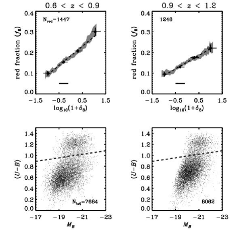
Figure 8.— As in Figure 3, except we plot the red fraction as a function of overdensity and the rest–frame color–magnitude distribution in only two distinct redshift ranges for the full galaxy sample (Sample A). Here, the redshift bins are selected to match those of Cucciati et al. (2006). In comparison to Figure 6 of Cucciati et al. (2006), we see a highly significant environment trend where they do not.

First of all, because rest–frame galaxy colors (which depend on photometry and coarsely on redshift) are almost entirely independent of the environment measurements (which depend upon angular positions and high–precision redshifts), we consider it unlikely that the highly significant correlation between red fraction and environment, which we find at $z\sim 1$, is false. It persists in all four samples considered here, which should differ from each other by more than sample B should differ from the VVDS volume–limited sample. Since there are few galaxies in the gap between the red and blue populations, modest differences in the definition of $f_{\rm R}$ have minimal effect, as well, so this is unlikely to explain any differences.

In an effort to conduct a more direct comparison between the VVDS and DEEP2 results, we attempt to replicate as closely as possible those VVDS subsamples for which we can establish a volume–complete DEEP2 analogue and apply to them the same red–fraction definition as employed by Cucciati et al. (2006). While in this paper we generally define the red fraction, $f_{\rm R}$, according to a color division in $U-B$ versus $M_{B}$ color–magnitude space, Cucciati et al. (2006) utilize a luminosity–independent selection in $u^{*}-g^{\prime}$. Using the CFHT/Megacam $u^{*}$ and $g^{\prime}$ filter response, quantum efficiency, telescope throughput, and atmospheric extinction estimates, the K–correction code (kcorrect version v4_1_2) of Blanton et al. (2003), and our CFHT $B,R,I$ photometry (Coil et al., 2004b), we compute the rest–frame $u^{*}-g^{\prime}$ color for each galaxy in the DEEP2 spectroscopic sample. Cucciati et al. (2006) divide samples according to Johnson/Cousins $B$–band absolute magnitude in the AB system, taking $h=1$; this is identical to the $M_{B}$ used throughout this paper (cf. §2.2). We are therefore able to place the DEEP2 galaxies in the same color–magnitude space as that of Cucciati et al. (2006) and define “red” according to the VVDS definition ($u^{*}-g^{\prime}\geq 1.1$).

In order to match the VVDS samples as closely as possible, we have constructed DEEP2 samples covering identical redshift regimes ($0.6<z<0.9$ and $0.9<z<1.2$) and absolute–magnitude limits ($M_{B}\leq-20,-20.5,-21$) as VVDS subsamples studied by Cucciati et al. (2006). Because of the differences between the DEEP2 $R$-band and VVDS $I$-band selections, it is possible to replicate only some of the VVDS subsamples. For $z<0.9$, we can construct volume–limited DEEP2 samples down to $M_{B}=-20$, while for $z<1.2$ we are able to construct a volume–limited sample matching the VVDS $M_{B}<-21$ data set, and a very nearly volume–limited sample with $M_{B}<-20.5$. Figures 7 and 8 of Cucciati et al. (2006) illustrate the red fraction versus overdensity trends for the corresponding samples drawn from VVDS.

As shown in Figure 9, the DEEP2 results — for volume–limited samples at $0.6<z<0.9$ and $0.9<z<1.2$ — are consistent with the VVDS results for similarly–selected data sets. However, the errors on the VVDS trends between red fraction and environment are significantly larger ($\gtrsim 2\times$ those for DEEP2). To make this figure, we map the data points from Figure 7 of Cucciati et al. (2006) onto the DEEP2 results by plotting the extreme-overdensity VVDS points at the same abcissa values as the extreme-overdensity DEEP2 points. This is necessary because citetcucciati06 measures environments over much larger scales than we do in DEEP2, and density contrasts on larger scales should be smaller. However, locally, at least, the same trends are found using environments measured on smaller and larger scales (Blanton et al., 2006).

No scaling, however, is applied to the VVDS red–fraction values, as plotted in Figure 9. The difference in normalization of $f_{\rm R}$ between DEEP2 and VVDS could be due to K–correction errors in either sample, or, conceivably, due to a possible tendency of VVDS to fail to obtain high–confidence redshifts for red galaxies as often as blue, especially at $z\gtrsim 1$. From this comparison to the Cucciati et al. (2006) results, we conclude that the color–density relation at $z>0.9$, as observed by DEEP2, is generally consistent with the VVDS measurements. However, due to their larger uncertainties (likely principally due to their smaller sample size), the color–density relation found here could not have been detected significantly by Cucciati et al. (2006).

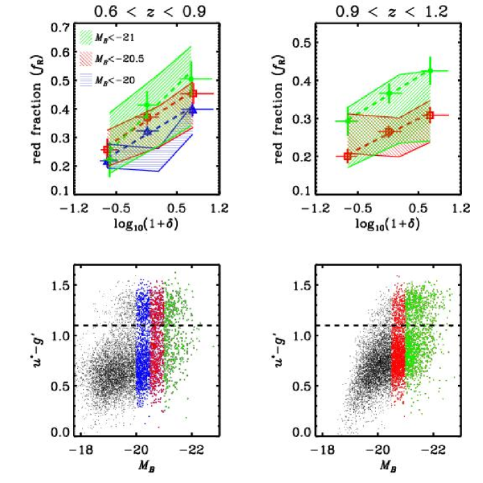
Figure 9.— As in Figure 3, except here we plot the red fraction as a function of overdensity, $\log_{10}(1+\delta_{3})$, in two distinct redshift ranges, $0.6<z<0.9$ and $0.9<z<1.2$. The green circles, red squares, and blue triangles correspond to volume–limited samples with $M_{B}<-21$, $-20.5$, and $-20$, respectively. The shaded (or filled) regions in each panel show the 1–$\sigma$ range of the red fraction as a function of overdensity for the corresponding VVDS samples, as plotted in Figure 7 of Cucciati et al. (2006); a key to the hatching patterns used is shown at upper left. As discussed in the text, the extreme–overdensity VVDS points have been mapped onto the corresponding extreme points from DEEP2, while the VVDS red fraction values remain unmodified. Bottom Row: We plot the rest–frame color–magnitude relation, $u^{*}-g^{\prime}$ versus $M_{B}$, for all DEEP2 objects in each redshift bin. The division between the red sequence and the blue cloud is given by the dashed line at $u^{*}-g^{\prime}=1.1$, following the definition of Cucciati et al. (2006). The various magnitude–limited samples, $M_{B}<-21$, $-20.5$, and $-20$, are denoted by the green, red, and blue colored symbols, respectively. Comparing like galaxy samples, the DEEP2 and VVDS results are generally in agreement, given the significantly larger errors for the Cucciati et al. (2006) data set.

Given that a perfect match between our samples and techniques and those of Cucciati et al. (2006) is impossible, especially due to the overdensity mapping applied in Figure 9, we also consider other possible reasons for why a trend present in DEEP2 could be missed within the VVDS data set. It is quite possible that fundamental differences in the samples observed could contribute to the differing conclusions at $z\sim 1$ from the DEEP2 and VVDS analyses. In particular, the VVDS sample includes a subset of objects to $I_{\rm AB}=24$, while DEEP2 samples down to a limit of $R_{\rm AB}=24.1$. As a consequence, while the surveys have comparable depths for the bluest objects, VVDS is deeper for red galaxies at $z>1$, which have $(R-I)_{AB}\sim 1$–$1.5$. As a result, Cucciati et al. (2006) include fainter red galaxies in their $f_{\rm R}$ measurements than we do in our standard samples (in the volume–limited subsamples, the respective depths are indentical, of course), and are able to study samples with color–independent $M_{B}$ limits down to $-19.5$ (for $z<1.2$). As shown in Fig. 9, however, volume–limited DEEP2 samples matching VVDS samples in luminosity range do exhibit a significant color–density trend where the equivalent VVDS samples do not.

In addition to the Cucciati et al. (2006) sample being small (6,582 galaxies) in comparison to our DEEP2 sample, yielding increased Poisson errors, it is also limited to a single $0.7^{\circ}\times 0.7^{\circ}$ field, which increases the uncertainties due to sample (or “cosmic”) variance compared to our sample. The differences between our results and those of Cucciati et al. (2006), however, are likely not attributable to cosmic variance alone. As shown in Figure 10, the variation in the $f_{\rm R}$–overdensity relation from field to field within the DEEP2 survey is small, with each field yielding a color–density relation consistent with that of the full sample. Cosmic variance mostly changes the overall red fraction in a given field and the relative abundance of the different environments, but not the strength of a trend.

In addition to smaller sample sizes, which yield larger errors in $f_{\rm R}$, there are other phenomena which could obscure a true correlation between red fraction and overdensity in VVDS data preferentially at high redshift. One possibility is that environment errors in the Cucciati et al. (2006) sample are large compared to their environment bins at $z>0.9$. We note that the 5%–95% range of measured overdensities increases with $z$ in their data set, as seen in Fig. 6 of Cucciati et al. (2006); this could reflect increasing errors in their environment measures (in the DEEP2 data set, in contrast, the 5%–95% range in measured overdensities is nearly independent of redshift).

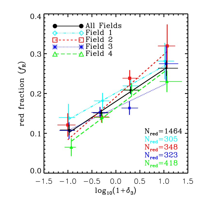
Figure 10.— Using the full galaxy sample (Sample A), we plot the red fraction as a function of overdensity, $\log_{10}{(1+\delta_{3})}$, at $0.8<z<1$ in each of the four DEEP2 fields. The data points give the red fraction as a function of the median overdensity computed in four distinct bins of $\log_{10}{(1+\delta_{3})}$. The horizontal error bars run from the twenty–fifth percentile to the seventy–fifth percentile of the overdensity distribution in each bin. The vertical error bars give the 1–$\sigma$ uncertainty on the red fraction within each overdensity bin, given by Poisson statistics. The lines show linear–regression fits to the data points in each field. In the bottom right corner of the plot, we give the number of red galaxies within the $0.8<z<1$ redshift range in each field. The field–to–field variance in the $f_{\rm R}$–overdensity correlation is small, illustrating the small uncertainty due to cosmic variance. Cosmic variance mostly changes the overall red fraction in a given field and the relative abundance of the different environments, but not the strength of a trend.

Another difference is that Cucciati et al. (2006) use a large smoothing kernel ($\sim\!5\ h^{-1}$ Mpc) in measuring environments. Estimating overdensities on such large scales can be problematic due to the small number of independent resolution elements across such a small field (at $z\sim 1$, $0.7^{\circ}$ corresponds to $\sim 30\ h^{-1}$ comoving Mpc) and due to the large percentage of the sample which falls within one smoothing scale length of a survey boundary or edge ($>\!50\%$ of the VVDS field by area at $z\sim 1$). Differences between the true relationship connecting color and environment on smaller scales and 5 Mpc scales (as used by Cucciati et al., 2006) could also account for discrepancies between DEEP2 and VVDS results, but at $z\sim 0$, at least, correlations between galaxy properties and environment measurements on $\sim 1$ and $\sim 8$ Mpc scales appear to differ significantly only in noise properties (Blanton et al., 2006).

Finally, another effect that could dilute the measurements of Cucciati et al. (2006) results from the fact that at $z\gtrsim 1$ — the redshift regime where a lack of a color–density relation is found in the Cucciati et al. (2006) data — the VVDS sample is dominated by lower–quality VVDS redshifts (${\rm flag}=2$, Ilbert et al., 2005). A number of tests have found that the ${\rm flag}=2$ redshifts have a nonnegligible error rate ($\sim 20\%$, O. Ilbert, private communication; C. Wolf, private communication; Le Fèvre et al., 2005a), which would cause sources to be included in the Cucciati et al. (2006) sample at $z>1$ incorrectly, with both erroneous K–corrections and erroneous overdensity measurements. This contamination would dilute any true correlation between rest–frame color and environment. In this paper, we use only higher–confidence DEEP2 redshifts, which have an overall failure rate below 2% based upon tests with repeated observations (Davis et al., 2006).

While the color–density results of Cucciati et al. (2006) differ when compared to the trends found in the full DEEP2 sample, a comparison of similar samples (cf. Fig. 9) illustrates that the DEEP2 and VVDS results are mostly in agreement where they overlap, given the significantly larger errors for the Cucciati et al. (2006) data set, which are likely due to the smaller VVDS sample size. The various sources of error discussed above (cf. §4.1) could also be at play, though the dominant uncertainty appears to be statistical in nature. Overall, both studies independently find that the color–density relation grows weaker with increasing redshift.

Although trends at $0.9<z<1.2$ are not significant for any of the VVDS samples, at lower redshift Cucciati et al. (2006) conclude that the color–density relation is stronger for brighter galaxies than faint ones. In contrast, we do not observe significant variations in the color–density trend for samples differing in $M_{B}$. That is, over the absolute–magnitude ranges probed in Fig. 9, the slope of the $f_{\rm R}$–overdensity relation exhibits no statistically significant dependence on luminosity in our measurements. The volume–limited subsamples in Fig. 9, however, are overlapping rather than independent in luminosity and only probe a limited range of $M_{B}$. Thus, the lack of significant luminosity dependence to the color–density relation within DEEP2 is not a strong statement. As shown by Cooper et al. (2006), the dependence of mean environment on luminosity and color is effectively separable at $z\sim 1$, which implies that the dependence of the color–density relation on luminosity should not be strong over the luminosity range covered by DEEP2.

Within the context of the larger picture of galaxy evolution, as discussed in §4.2, a luminosity dependence to the evolution of the color–density relation may well exist. Comparison of our results and those of clustering studies at $z\sim 1$ (e.g., Coil et al., 2004a, b) to clustering measurements of bright galaxies at $z\sim 2$ (e.g., Quadri et al., 2006) lead to similar conclusions. As explained by Cucciati et al. (2006), such a result can be easily understood as an example of cosmic “downsizing” (Cowie et al., 1996), where the cessation of star formation occurs first in high–luminosity galaxies or high–mass halos (i.e., high–density environments). However, the methods used in this paper do not detect this trend within the DEEP2 data set.

4.2. Implications of the Observed Evolution in $f_{\rm R}(z)$

A quite striking result from our work is the difference between the evolution of the red fraction in under– and overdense environments spanning the redshift range $0.75<z<1.3$; while $f_{\rm R}$ in underdense environments remains roughly constant with $z$ in our sample, we find that the red fraction in dense environments decreases with $z$, such that it is roughly equal to the fraction in underdense environments at $z\sim 1.3$. Studying the properties of group galaxies in DEEP2, Gerke et al. (2006) find similar evolution in the color–density relation from $0.7\lesssim z\lesssim 1.3$, with the fraction of blue galaxies in groups becoming comparable to that of the field at $z\sim 1.3$. Given $\sim 1$ Gyr to move from the blue cloud to the red sequence (e.g., van Dokkum & Franx, 2001; Balogh et al., 2004b), if the color–density relation first arises at $z\sim 1.35$, then the physical mechanisms responsible must start to become operative at $z\sim 1.7$ within a concordance cosmology.

This observed evolution in the color–density relation and the existence of an epoch at which environment–dependent quenching initiates are both consistent with the current theoretical picture in which the conversion of blue galaxies into members of the red sequence occurs in dark matter halos with mass greater than some critical value $(\sim{\rm a\ few}\times 10^{11}\ {\rm M}_{\sun})$. As halos pass this mass threshold in such hot–flow/cold–flow accretion models, the infalling cold gas supply to the central galactic disk is virial shocked and shut off such that the galaxy will quickly burn its remaining fuel and redden (e.g., Birnboim & Dekel, 2003; Kereš et al., 2005). Within the models of Croton et al. (2006) and others (see also Bower et al., 2006; Cattaneo et al., 2006; Kang et al., 2006), low–energy AGN activity is included to suppress the cooling of shocked gas and the recommencement of star formation.

At yet higher redshifts $(z\gtrsim 2)$, even in halos above this critical threshold, quenching does not occur since cooling is effectively able to remove the pressure support behind the virial shock (Birnboim & Dekel, 2003). At later times, the evolution of the halo mass function (Jenkins et al., 2001; Springel et al., 2005) in combination with the near redshift–independence of the critical mass (Kereš et al., 2005; Croton et al., 2006; Cattaneo et al., 2006) leads to a continual increase in the number of halos above the threshold mass. Given the correlation between halo mass and environment in simulations (e.g., Lemson & Kauffmann, 1999; Maulbetsch et al., 2006; Wetzel et al., 2006), this thereby predicts an evolution in the color–density relation (i.e., becoming stronger) at $z\lesssim 1.3$. In this picture, the color–density or morphology–density relation within cluster environments likely persists out to higher redshifts, as cluster galaxies reside in the most massive halos, those first to reach the critical mass at $z\sim 2$. As DEEP2 primarily samples the more common, less massive groups, the color–density relation is still weak at somewhat later times, $z\sim 1.3$.

In addition to predicting evolution of the color–density relation at $z<1.3$, these hot–flow/cold–flow accretion models also provide an additional mechanism by which to explain the presence of red galaxies residing in underdense regions (cf. §3.2). While passive evolution or merging of several smaller galaxies to form a fossil group are also viable physical mechanisms by which to create such galaxies, the tail (at $\gtrsim{\rm a\ few}\times 10^{11}\ {\rm M}_{\sun}$) of the halo mass function in low–density environments naturally leads to the existence of at least some true red–sequence galaxies in voids.

The measured evolution in the color–density relation as presented here should be directly related to measurements of galaxy clustering at high redshift. We predict that the clustering of $\sim L^{*}$ galaxies at $z\gtrsim 1.3$ should depend only weakly on color. Studies of galaxy clustering by spectral type or by color at high redshift (e.g., Coil et al., 2004a, b; Meneux et al., 2006) have shown that blue, star–forming galaxies at $z\sim 1$ are less strongly clustered than their red counterparts. Such clustering work, however, spans a broad redshift range (extending to redshifts less than unity) and the galaxy samples utilized are dominated in number by galaxies at $z<1.2$, where we still find a significant color–density relation. Unfortunately, the DEEP2 sample includes a modest number of galaxies $(\sim 5000)$ at $z>1.2$, with very few on the red sequence; we therefore lack the statistical power needed to compute correlation strengths for subsamples by galaxy color at such redshifts.

At yet higher redshifts $(z\gtrsim 2)$ there are indications that clustering depends on color. Studies of UV–selected galaxies and red, near–IR bright galaxies have found significant differences in clustering strengths depending on the sample selection, with the latter being more strongly clustered (e.g., Daddi et al., 2003; Adelberger et al., 2005b; Foucaud et al., 2006). Furthermore, within near–IR bright samples, the measured correlation length depends significantly on apparent color (e.g., $R_{\rm AB}-K_{\rm Vega}$ or $J-K$), such that blue near–IR bright galaxies cluster like UV–selected Lyman–break galaxies (LBGs), while the red near–IR bright galaxies exhibit a correlation length larger by a factor of roughly two (Adelberger et al., 2005a; Quadri et al., 2006).

The red, near–IR bright samples observed at early epochs, however, are likely the antecedents of the rarest, most massive red galaxies today and are not representative of the progenitors of DEEP2 galaxies; their correlation length at $z\gtrsim 2$ already exceeds that of the brightest and reddest DEEP2 galaxy samples. Presumably, if we were to study similarly extreme samples at $z\sim 1.3$ (e.g., galaxies in massive clusters analogous to the candidates studied by Rosati et al., 2004; Mei et al., 2006a, b; Bremer et al., 2006), we should find a significant color–density relation. Instead, the progenitors of DEEP2 galaxies were bluer and/or fainter at $z\sim 2$ and resembled the LBGs more than those red galaxies which are most readily observed at high redshift.

Thus, our observations of the evolution of the red fraction in low–density and high–density environments do not contradict the current set of clustering measurements at higher redshift $(z\sim 2)$ or observations of massive clusters at $z>1$. Like the cluster galaxies, the red, near–IR selected, massive galaxies seen at high $z$, given their observed clustering, are likely to reside in very massive halos, which should be the first halos to cross the threshold quenching mass. In fact, estimates of their star–formation rates indicate that they are actively forming stars in large quantities (Daddi et al., 2004); hence, they do not appear to generally have been quenched at $z\sim 2$, though more recent observations of near–IR selected galaxies at $z\sim 2$ indicate relatively low star–formation activity in at least a portion of the massive galaxy population at high redshift (Labbé et al., 2005; Kriek et al., 2006).

5. Summary & Conclusions

In this paper, we present a detailed study of the evolution in the color–density relation at $0.4<z<1.35$. Using a sample of galaxies drawn from the DEEP2 Galaxy Redshift Survey, we estimate the local overdensity about each galaxy according to the projected $3^{\rm rd}$–nearest–neighbor surface density. From this, we measure the evolution of the red fraction with environment across time. Our principal results are as follows:

• We find that the color–density relation observed locally still exists at $z>1$; the fraction of galaxies on the red sequence increases with local galaxy overdensity to nearly the redshift limits of the DEEP2 survey.

• At all epochs probed $(0.4<z<1.3)$, we find there exists a population of red, morphologically early–type galaxies residing in the the most underdense environments.

• The color–density relation evolves with redshift, growing weaker with lookback time such that at $z\gtrsim 1.3$ there is no detectable dependence of galaxy color on local environment in the DEEP2 sample.

• Our results support a picture in which the red sequence grew preferentially in dense environments (i.e., galaxy groups) at $z\lesssim 1.5$. Clearly, the local environment plays an important role in “nurturing” galaxies, establishing the existence of correlations such as the morphology–density and color–density relation over cosmic time. The strength of evolutionary trends suggests that the correlations observed locally do not appear to have been imprinted (by “nature”) upon the galaxy population during their epoch of formation.

• Our findings imply that there should be little color dependence in the clustering of $\sim L^{*}$ galaxies at $z\gtrsim 1.3$.

References

- Adelberger et al. (2005a) Adelberger, K. L., Erb, D. K., Steidel, C. C., Reddy, N. A., Pettini, M., & Shapley, A. E. 2005a, ApJ, 620, L75
- Adelberger et al. (2005b) Adelberger, K. L., Steidel, C. C., Pettini, M., Shapley, A. E., Reddy, N. A., & Erb, D. K. 2005b, ApJ, 619, 697
- Baldry et al. (2004) Baldry, I. K., Glazebrook, K., Brinkmann, J., Ivezić, Ž., Lupton, R. H., Nichol, R. C., & Szalay, A. S. 2004, ApJ, 600, 681
- Balogh et al. (2004a) Balogh, M. et al. 2004a, MNRAS, 348, 1355
- Balogh et al. (2004b) Balogh, M. L., Baldry, I. K., Nichol, R., Miller, C., Bower, R., & Glazebrook, K. 2004b, ApJ, 615, L101
- Balogh et al. (1997) Balogh, M. L., Morris, S. L., Yee, H. K. C., Carlberg, R. G., & Ellingson, E. 1997, ApJ, 488, L75+
- Barnes & Hernquist (1992) Barnes, J. E. & Hernquist, L. 1992, ARA&A, 30, 705
- Bell et al. (2004) Bell, E. F. et al. 2004, ApJ, 608, 752
- Birnboim & Dekel (2003) Birnboim, Y. & Dekel, A. 2003, MNRAS, 345, 349
- Blanton (2006) Blanton, M. R. 2006, ApJ, 648, 268
- Blanton et al. (2006) Blanton, M. R., Eisenstein, D., Hogg, D. W., & Zehavi, I. 2006, ApJ, 645, 977
- Blanton et al. (2005) Blanton, M. R., Eisenstein, D., Hogg, D. W., Schlegel, D. J., & Brinkmann, J. 2005, ApJ, 629, 143
- Blanton et al. (2003) Blanton, M. R. et al. 2003, AJ, 125, 2348
- Bower et al. (2006) Bower, R. G. et al. 2006, MNRAS, accepted [astro-ph/0511338]
- Bremer et al. (2006) Bremer, M. N. et al. 2006, MNRAS, accepted [astro–ph/0607425]
- Cattaneo et al. (2006) Cattaneo, A. et al. 2006, MNRAS, submitted [astro-ph/0605750]
- Coil et al. (2004a) Coil, A. L. et al. 2004a, ApJ, 609, 525
- Coil et al. (2004b) —. 2004b, ApJ, 617, 765
- Coil et al. (2004b) —. 2006b, ApJ, 644, 671
- Colless et al. (2001) Colless, M. et al. 2001, MNRAS, 328, 1039
- Colless et al. (2003) —. 2003, VizieR Online Data Catalog, 7226, 0
- Cooper et al. (2005) Cooper, M. C., Newman, J. A., Madgwick, D. S., Gerke, B. F., Yan, R., & Davis, M. 2005, ApJ, 634, 833
- Cooper et al. (2006) Cooper, M. C. et al. 2006, MNRAS, 370, 198
- Couch et al. (1998) Couch, W. J., Barger, A. J., Smail, I., Ellis, R. S., & Sharples, R. M. 1998, ApJ, 497, 188
- Cowie et al. (1996) Cowie, L. L., Songaila, A., Hu, E. M., & Cohen, J. G. 1996, AJ, 112, 839
- Croton et al. (2005) Croton, D. J. et al. 2005, MNRAS, 356, 1155
- Croton et al. (2006) —. 2006, MNRAS, 365, 11
- Cucciati et al. (2006) Cucciati, O. et al. 2006, A&A, 458, 39
- Daddi et al. (2003) Daddi, E. et al. 2003, ApJ, 588, 50
- Daddi et al. (2004) —. 2004, ApJ, 600, L127
- Davis & Geller (1976) Davis, M. & Geller, M. J. 1976, ApJ, 208, 13
- Davis et al. (2003) Davis, M. et al. 2003, in Discoveries and Research Prospects from 6- to 10-Meter-Class Telescopes II. Edited by Guhathakurta, Puragra. Proceedings of the SPIE, Volume 4834, pp. 161-172 (2003)., 161–172
- Davis et al. (2006) Davis, M. et al. 2006, ApJ, in preparation
- Dressler (1980) Dressler, A. 1980, ApJ, 236, 351
- Dressler et al. (1997) Dressler, A. et al. 1997, ApJ, 490, 577
- Ellis et al. (1997) Ellis, R. S., Smail, I., Dressler, A., Couch, W. J., Oemler, A., Jr., Butcher, H., & Sharples, R. M. 1997, ApJ, 483, 582
- Faber et al. (2005) Faber, S. M. et al. 2005, ApJ, submitted
- Faber et al. (2006) —. 2006, ApJ, in preparation
- Foucaud et al. (2006) Foucaud, S. et al. 2006, MNRAS, submitted [astro-ph/0606386]
- Gerke et al. (2006) Gerke, B. F. et al. 2006, ApJ, in preparation
- Hopkins et al. (2005) Hopkins, P. F., Hernquist, L., Cox, T. J., Di Matteo, T., Martini, P., Robertson, B., & Springel, V. 2005, ApJ, 630, 705
- Ilbert et al. (2005) Ilbert, O. et al. 2005, A&A, 439, 863
- Jenkins et al. (2001) Jenkins, A., Frenk, C. S., White, S. D. M., Colberg, J. M., Cole, S., Evrard, A. E., Couchman, H. M. P., & Yoshida, N. 2001, MNRAS, 321, 372
- Kang et al. (2006) Kang, X., Jing, Y. P., & Silk, J. 2006, ApJ, 648, 820
- Kauffmann et al. (2004) Kauffmann, G., White, S. D. M., Heckman, T. M., Ménard, B., Brinchmann, J., Charlot, S., Tremonti, C., & Brinkmann, J. 2004, MNRAS, 353, 713
- Kereš et al. (2005) Kereš, D., Katz, N., Weinberg, D. H., & Davé, R. 2005, MNRAS, 363, 2
- Kormendy & Fisher (2005) Kormendy, J. & Fisher, D. B. 2005, in Revista Mexicana de Astronomia y Astrofisica Conference Series, 101–108
- Kriek et al. (2006) Kriek, M. et al. 2006, ApJ, 649, 71
- Labbé et al. (2005) Labbé, I. et al. 2005, ApJ, 624, 81
- Le Fèvre et al. (2005a) Le Fèvre, O. et al. 2005a, Nature, 437, 519
- Le Fèvre et al. (2005b) —. 2005b, A&A, 439, 845
- Lemson & Kauffmann (1999) Lemson, G. & Kauffmann, G. 1999, MNRAS, 302, 111
- Lotz et al. (2006) Lotz, J. M. et al. 2006, ApJ, submitted [astro-ph/0602088]
- Madgwick et al. (2002) Madgwick, D. S. et al. 2002, MNRAS, 333, 133
- Madwgick et al. (2003) Madwgick, D. S. et al. 2003, MNRAS, 344, 847
- Martínez et al. (2006) Martínez, H. J., O’Mill, A. L., & Lambas, D. G. 2006, MNRAS, 372, 253
- Maulbetsch et al. (2006) Maulbetsch, C., Avile-Reese, V., Colin, P., Gottloeber, S., Khalatyan, A., & Steinmetz, M. 2006, ApJ, submitted [astro-ph/0606360]
- Mei et al. (2006a) Mei, S. et al. 2006a, ApJ, 639, 81
- Mei et al. (2006b) —. 2006b, ApJ, 644, 759
- Menanteau et al. (2006) Menanteau, F., Ford, H. C., Motta, V., Benítez, N., Martel, A. R., Blakeslee, J. P., & Infante, L. 2006, AJ, 131, 208
- Meneux et al. (2006) Meneux, B. et al. 2006, A&A, 452, 387
- Navarro et al. (1987) Navarro, J. F., Mosconi, M. B., & Lambas, D. G. 1987, MNRAS, 228, 501
- Nuijten et al. (2005) Nuijten, M. J. H. M., Simard, L., Gwyn, S., & Röttgering, H. J. A. 2005, ApJ, 626, L77
- Oemler (1974) Oemler, A. J. 1974, ApJ, 194, 1
- Oke & Gunn (1983) Oke, J. B. & Gunn, J. E. 1983, ApJ, 266, 713
- Peacock & Smith (2000) Peacock, J. A. & Smith, R. E. 2000, MNRAS, 318, 1144
- Poggianti et al. (2006) Poggianti, B. M. et al. 2006, ApJ, 642, 188
- Postman et al. (2005) Postman, M. et al. 2005, ApJ, 623, 721
- Quadri et al. (2006) Quadri, R. et al. 2006, ApJ, submitted [astro-ph/0606330]
- Rojas et al. (2005) Rojas, R. R., Vogeley, M. S., Hoyle, F., & Brinkmann, J. 2005, ApJ, 624, 571
- Rosati et al. (2004) Rosati, P. et al. 2004, AJ, 127, 230
- Seljak (2000) Seljak, U. 2000, MNRAS, 318, 203
- Smith et al. (2005) Smith, G. P., Treu, T., Ellis, R. S., Moran, S. M., & Dressler, A. 2005, ApJ, 620, 78
- Springel et al. (2005) Springel, V. et al. 2005, Nature, 435, 629
- Stanford et al. (1998) Stanford, S. A., Eisenhardt, P. R., & Dickinson, M. 1998, ApJ, 492, 461
- Strateva et al. (2001) Strateva, I. et al. 2001, AJ, 122, 1861
- Toomre & Toomre (1972) Toomre, A. & Toomre, J. 1972, ApJ, 178, 623
- Treu et al. (2003) Treu, T., Ellis, R. S., Kneib, J.-P., Dressler, A., Smail, I., Czoske, O., Oemler, A., & Natarajan, P. 2003, ApJ, 591, 53
- van Dokkum & Franx (2001) van Dokkum, P. G. & Franx, M. 2001, ApJ, 553, 90
- van Dokkum et al. (2000) van Dokkum, P. G., Franx, M., Fabricant, D., Illingworth, G. D., & Kelson, D. D. 2000, ApJ, 541, 95
- Vogt et al. (2005) Vogt, N. P. et al. 2005, ApJS, 159, 41
- Weiner et al. (2005) Weiner, B. J. et al. 2005, ApJ, 620, 595
- Wetzel et al. (2006) Wetzel, A. R., Cohn, J. D., White, M., Holz, D. E., & Warren, S. 2006, ApJ, submitted [astro-ph/0606699]
- Willmer et al. (2006) Willmer, C. N. A. et al. 2006, ApJ, 647, 853
- Wolf et al. (2001) Wolf, C., Dye, S., Kleinheinrich, M., Meisenheimer, K., Rix, H.-W., & Wisotzki, L. 2001, A&A, 377, 442
- Wolf et al. (2003) Wolf, C., Meisenheimer, K., Rix, H.-W., Borch, A., Dye, S., & Kleinheinrich, M. 2003, A&A, 401, 73
- Yan et al. (2003) Yan, R., Madgwick, D. S., & White, M. 2003, ApJ, 598, 848
- Yan et al. (2004) Yan, R., White, M., & Coil, A. L. 2004, ApJ, 607, 739
- Yang et al. (2003) Yang, X., Mo, H. J., & van den Bosch, F. C. 2003, MNRAS, 339, 1057
- Yee et al. (2005) Yee, H. K. C., Hsieh, B. C., Lin, H., & Gladders, M. D. 2005, ApJ, 629, L77
- York et al. (2000) York, D. G. et al. 2000, AJ, 120, 1579
- Zhang (1996) Zhang, X. 1996, ApJ, 457, 125