A Time Delay for the Largest Gravitationally Lensed Quasar: SDSS J1004+4112

Abstract

We present 426 epochs of optical monitoring data spanning 1000 days from December 2003 to June 2006 for the gravitationally lensed quasar SDSS J1004+4112. The time delay between the A and B images is $\Delta t_{\mathrm{BA}}=38.4\pm 2.0$ days ($\Delta\chi^{2}=4$) in the expected sense that B leads A and the overall time ordering is C-B-A-D-E. The measured delay invalidates all published models. The models failed because they neglected the perturbations from cluster member galaxies. Models including the galaxies can fit the data well, but strong conclusions about the cluster mass distribution should await the measurement of the longer, and less substructure sensitive, delays of the C and D images. For these images, a delay of $\Delta t_{\mathrm{CB}}\simeq 681\pm 15$ days is plausible but requires confirmation, while delays of $\Delta t_{\mathrm{CB}}>560$ days and $\Delta t_{\mathrm{AD}}>800$ days are required. We clearly detect microlensing of the A/B images, with the delay-corrected flux ratios changing from $m_{B}-m_{A}=0.44\pm 0.01$ mag in the first season to $0.29\pm 0.01$ mag in the second season and $0.32\pm 0.01$ mag in the third season.

1 Introduction

The wide-separation lensed quasar SDSS J1004+4112 was discovered in the Sloan Digital Sky Survey search for lenses (Inada et al. 2003; Oguri et al. 2004; Sharon et al. 2005; Wambsganss 2003). The lens consists of at least four images of a redshift $z_{s}=1.734$ quasar whose $\sim 15\farcs 0$ Einstein ring diameter is created by a redshift $z_{l}=0.68$ cluster. The cluster has been characterized with X-ray observations (Ota et al. 2006) and there are additional multiply imaged arcs formed from still higher redshift background galaxies (Sharon et al. 2005). There is also strong evidence for a fifth, lensed image of the quasar located near the center of the brightest cluster galaxy (Inada et al. 2005), which in combination with a future velocity dispersion measurement for the galaxy will strongly constrain the central mass distribution of the lens (e.g. Sand et al. 2002, but see Dalal & Keeton 2003). Thus, it is not only feasible to cleanly compare X-ray and lensing mass distributions in this galaxy cluster, but it may also be possible to test the cosmological model by measuring the increase of the Einstein radius with source redshift due to the $D_{LS}/D_{OS}$ distance ratio scaling of the lens deflection (Soucail et al. 2004).

That the source is a time-variable quasar offers further and unique opportunities for this cluster lens. First, the time delay between the quasar images can be measured as a constraint on the mass distribution. In theory, the time delays determine the mean surface density near the images for which the delay is measured (Kochanek 2002), so the mass sheet ($\kappa$) degeneracy of most cluster lensing measurements can be broken under the assumption that the Hubble constant is well-determined by other means. Several theoretical studies of the time delays in SDSS J1004+4112 (Oguri et al. 2004; Williams & Saha 2004; Kawano & Oguri 2006) have explored their dependence on the mean mass profile of the cluster, finding a broad range of potential delays. As we shall see, all these models are incorrect in their details because they neglected cluster member galaxies whose deflection scales are larger than the positional constraints on the quasar images used in the models (see the discussion in Keeton et al. 2000 on the failure of similar models for the cluster lens Q0957+561 and the general discussion in Kochanek 2005). Nonetheless, all these models indicate that the delay between the A and B images is relatively short (weeks) and that its value should indicate the magnitude of the much longer (years) delays of the C and D images.

The second unique property of the lens is that microlensing of the quasar accretion disk by any stars in the cluster halo or small satellites near the images can be used as an added probe of the structure of the cluster (see Wambsganss 2006). Because the cluster has a higher velocity dispersion ($700$ km/s) than a typical galaxy lens ($\sim 200$ km/s), the microlensing time scales in this system may also be shorter than for a lens by about a factor of 3. There is already evidence for microlensing from the time variability of the C IV 1549Å line in image A that is not observed in image B (Richards et al. 2004, Lamer et al. 2006, Gómez-Álvarez et al. 2006), although recently Green (2006) has suggested that this could also be due to time variable absorption in the source quasar.

For three years we have conducted an optical monitoring campaign to measure the optical variability of this system. This has proved more challenging than desired because the quasars are somewhat faint for monitoring with available telescopes and modest exposure times. However, we have succeeded both in measuring the A/B time delay and clearly detecting microlensing of the optical continuum of the quasar. In §2 we present the data from the monitoring campaign for the four bright lensed quasar images. In §3 we determine the A/B time delay, discuss the presence of microlensing in the system, and place constraints on the long delays between the close image pair A and B and the fainter images C and D. In §4 we discuss the failure of existing models for the system and introduce a simple successful model that includes the perturbations of cluster galaxies, and we conclude in §5.

2 Data

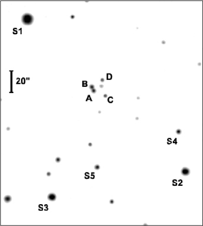
Figure 1: The r-band image obtained with Minicam on January 16, 2005. The 3.3 arcmin $\times$ 3.5 arcmin field shows the lensed images of SDSS J1004+4112 and the five reference stars S1, S2, S3, S4 and S5 used for the PSF.

The photometric monitoring observations presented here took place between December 2003 and June 2006. The bulk of data were taken with the 1.2m telescope at Fred Lawrence Whipple Observatory on Mount Hopkins using the 4Shooter (R-band, 93 epochs, 0$\farcs$66 pixels), Minicam (SDSS r-band, 74 epochs, 0$\farcs$604 pixels), and Keplercam (SDSS r-band, 91 epochs, 0$\farcs$672 pixels, plus 4 epochs in R-band) during the first, second and third season, respectively. Additional data were obtained with the Apache Point Observatory (APO) 3.5m telescope using SPICam (SDSS r-band, 9 epochs, 0$\farcs$282 pixels), the MDM 2.4m Hiltner telescope using the RETROCAM (Morgan et al. 2005, SDSS r-band, 27 epochs, 0$\farcs$259 pixels), 8K (R-band, 12 epochs, 0$\farcs$344 pixels), Templeton (R-band, 8 epochs, 0$\farcs$275 pixels) and Echelle (R-band, 3 epochs, 0$\farcs$275 pixels) detectors, the MDM 1.3m McGraw-Hill telescope using the Templeton detector (R-band, 6 epochs, 0$\farcs$508 pixels), the Palomar Observatory 1.5m telescope using the SITe detector (R-band, 13 epochs, 0$\farcs$379 pixels), the Wise Observatory 1.0m telescope with the Tektronix (R-band, 30 epochs, 0$\farcs$696 pixels) and TAVAS (clear, 53 epochs, 0$\farcs$991 pixels) detectors, and the WIYN 3.5m telescope using the WTTM (SDSS r-band, 3 epochs, 0$\farcs$216 pixels) detector. The combined data set consists of 426 epochs.

In Figure 1 the quasar images are labeled A, B, C and D, following the notation by Inada et al. (2003). The (non-variable) reference stars used for flux calibration and building the PSF are S1, S2, S3, S4 and S5. The small panels in Figure 2 show snapshots of the four bright quasar images at three different observing epochs, in March 2004, May 2005 and March 2006. These images illustrate how images A and B slowly faded during the course of the three seasons, while image D became significantly brighter. The galaxies of the lensing cluster are not detectable in the individual observations, except for the bright galaxy close to image D (G1 in Oguri et al. 2004). The candidate fifth quasar image, E, lies near the center of this galaxy (Inada et al. 2005).

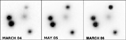
Figure 2: The panels show $23\arcsec\times~{}23\arcsec$ insets on the four bright quasar images at three different epochs separated by about one year (for nomenclature cf. Fig. 1). The faint image in their middle is the bright galaxy belonging to the lensing cluster.

The data were fitted using the methods of Kochanek et al. (2006) for HE 0435–1223. Regions around each of the quasar images and the “standard” S1-S5 stars (see Fig. 1) are fitted to determine the relative fluxes and the structure of the PSF. For each filter, the star S1 was defined to have unit flux while the fluxes of the remaining stars S2, S3, S4 and S5 were adjusted to this calibration standard based on all the available epochs of data for each filter. The relative fluxes of the standard stars depend on the filter, with ratios of 1.0:0.439:0.360:0.130:0.0583 for the R-band, 1.0:0.334:0.329:0.0937:0.0613 for the SDSS r-band, and 1.0:0.63:0.64:0.39:0.20 for the clear filter. In the WIYN/WTTM, MDM 2.4m/8K and MDM 2.4m/Templeton data, the star S1 frequently is too close to saturation for use, so its weight in the fits is greatly reduced. It was not necessary to further subdivide the calibrations for the individual detectors given the overall quality of the photometry, as the average calibration offsets between detectors were well under 0.01 mag. We then matched the R-band and clear observations to the r-band observations using the quasar light curves themselves. For each R/clear epoch bracketed by r-band observations within 1 week, we interpolated the r-band observation to the epoch of the other band and computed the mean offset between the light curves. Offsets of $0.043\pm 0.006$ mag and $0.250\pm 0.011$ mag must be added to the R-band and clear magnitudes respectively to match them to the r-band data.

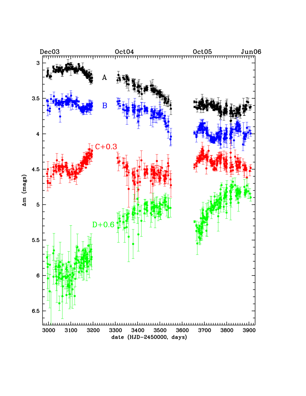
Figure 3: Light curves of the A-D images of SDSS J1004+4112 from December 2003 to June 2006. Images C and D have been offset by 0.3 and 0.6 mag because they would otherwise overlap with each other and with image B in the third season.

Figure 3 shows the resulting light curves for images A–D over the three observing seasons and Table 1 presents the photometry for images A and B. They span a time period of 1000 days from December 2003 to June 2006 with two seasonal gaps of approximately 100 days during the period from July to October. SDSS J1004+4112 is a relatively faint quasar for monitoring with 1m-class telescopes, and the image quality of the FLWO and WISE telescopes is poor. As a result, the noise in many of the measurements is relatively large compared to the variability amplitude. On the other hand, our sampling cadence is quite high, so the overall statistical power of the data is very good, with a mean sampling rate of once every two days while the source is visible. All four images vary by about 0.5 mag, with the more than 1 mag brightening of image D being the largest change during the three seasons. For the purposes of measuring the A/B time delay, the most interesting features are the minima in the B light curve near days $3150$ and $3750$ in the first and third seasons respectively, and the corresponding features in the A light curve roughly 40 days later. The second season shows no obvious features that can be used to measure the delay. The second important point to note is that the A/B flux ratio has changed significantly between the first and third seasons, indicating that microlensing is occurring in this system as has been previously suggested by variations in the C IV emission line profile (Richards et al. 2004, Lamer et al. 2006, Gómez-Álvarez et al. 2006).

3 The Time Delay

Model predictions for the time delay of the close image pair A and B are a few weeks (Oguri et al. 2004; Williams $\&$ Saha 2004, Kawano & Oguri 2006) and therefore should be measurable within each season of the light curves. Of the many techniques for calculating time delays from light curves (e.g. Gil-Merino et al. 2002, Pelt et al. 1994, Press, Rybicki & Hewitt 1992, Kochanek et al. 2006), we will apply three. The three methods produce mutually consistent results, but we will adopt the Kochanek et al. (2006) polynomial method for our standard result because it naturally includes the effects of microlensing on the delay estimate. As is clear from the light curves, image B leads image A, so the delay ordering of the images is C-B-A-D-E. We conclude with a discussion of the longer C and D image time delays.

For our analysis of the A/B delay we treated the data in Table 1 as follows. If the goodness of fit of the photometric model to an image had a $\chi^{2}$ statistic larger than the number of degrees of freedom $N_{dof}$ (see Table 1), we rescaled the photometric errors for that image by $\left(\chi^{2}/N_{dof}\right)^{1/2}$ on the grounds that having $\chi^{2}>N_{dof}$ meant that the uncertainties were underestimated. For the time delay estimates we dropped the 16 points marked in Table 1 that were more than $3\sigma$ from the best fitting models. We also repeated the time delay estimates excluding all points with rescaled photometric errors larger than $0.1$ mag, finding no significant changes.

3.1 Simple $\chi^{2}$ minimization

The simplest approach to the delay measurement problem is to take the observed light curves $A(t_{i})$ and $B(t_{i})$ and cross-correlate them with linearly interpolated light curves $a(t)$ and $b(t)$ for the other image. We assume that that the light curves of the two images are the same except for a time delay $\tau$ and a magnitude offset $m(\tau)$. In practice, we use a different magnitude offset for each season to partially compensate for the effects of microlensing. Based on this assumption we can calculate the time delay by minimizing the deviations from $m(\tau)$ for each pair $(A(t_{i}),b(t_{i}-\tau))$ and $(a(t_{i}+\tau),B(t_{i}))$ by a fit statistic

$${\chi^{2}(\tau)\over N_{dof}(\tau)} ={1\over 2N_{dof}(\tau)}\sum\limits^{N(\tau)}_{i}{(A(t_{i})-b(t_{i}-\tau)+m(\tau))^{2}\over\sigma_{A,i}^{2}+\sigma_{b,t}^{2}}$$ (1)

$$+{1\over 2N_{dof}(\tau)}\sum\limits^{N(\tau)}_{i}{(a(t_{i}+\tau)-B(t_{i})+m(\tau))^{2}\over\sigma_{a,t}^{2}+\sigma_{B,i}^{2}}$$

that is symmetric as to which image is being interpolated. The errors in the observed magnitudes are $\sigma_{A,i}$ and $\sigma_{B,i}$ and the errors in the interpolated magnitudes are $\sigma_{a,t}$ and $\sigma_{b,t}$. The fit is carried out only where the light curves overlap (i.e. excluding the season gaps), so the number of data points used $N(\tau)$ depends on the delay $\tau$.

Fig. 4 shows the results for the three seasons separately and for the combined light curve. Analyzed separately, the first and third seasons show minima at 31 and 40 days respectively, while there is no clear minimum for the second season due to the lack of significant features in the light curve. For the joint analysis of all three seasons we allowed for an independent value of $m(\tau)$ within each season to model the changes in the flux ratios due to microlensing. The analysis of the combined data yields a delay of 41$\pm$5 days.

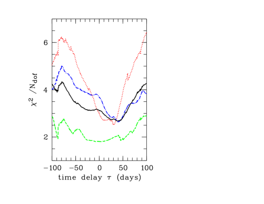
Figure 4: Results of the $\chi^{2}$ minimization between the two time series A and B for the first (red dotted line), second (green dashed line), third (blue dash-dotted line) and combined observing seasons (black solid line).

3.2 The Dispersion Method

One potential weakness of the simple $\chi^{2}$ method is the need for interpolation. As our second approach we apply the dispersion spectra method developed by Pelt et al. (1994, 1996) to avoid the interpolation. Instead, a combined light curve $C(t)$ is constructed by shifting the data points of one image in magnitude ($m(\tau)$) and time ($\tau$) and combining them with the data points of the other image

$$C(t_{k})=\left\{\begin{array}[]{l @{\quad{\mbox{if}}\quad} l}A_{i},&t_{k}=t_{i}\\ B_{j}-m(\tau),&t_{k}=t_{j}+\tau\\ \end{array}\right.$$ (2)

where $k=1,..,N$ and $N=N_{A}+N_{B}$. The time delay $\tau$ is estimated by minimizing the dispersion spectrum

$$D^{2}(\tau)=\min_{m(\tau)}{\sum\limits_{k=1}^{N-1}S_{k}W_{k}G_{k}(C_{k+1}-C_{k})^{2}\over 2~{}\sum\limits^{N-1}_{k=1}S_{k}W_{k}G_{k}}$$ (3)

where the $W_{k}=(\sigma_{k}^{2}+\sigma_{k+1}^{2})^{-1}$ are the statistical weights of the data, $G_{k}=1$ if the points $k$ and $k+1$ come from different images (A/B) and $G_{k}=0$ otherwise (A/A or B/B), and $S_{k}=1$ if $|t_{k+1}-t_{k}|\leq\delta$ and $S_{k}=0$ otherwise. We use a decorrelation time scale of $\delta=3$ days, but our results depend little on the exact choice. The results are shown in Figure 5 for both the individual seasons and the combined data. We again used independent estimates of $\Delta m$ for each observing season to compensate for the effects of microlensing. We find $34$ and $39$ days for the first and third seasons, $39$ days for the combined data, and no significant minimum using only the data from the second season.

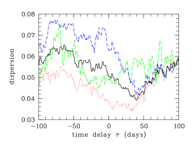
Figure 5: Dispersion spectra for the first (red dotted line), second (green dashed line), third (blue dash-dotted line) and combined observing seasons (black solid line).

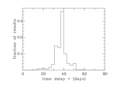
Figure 6: Results of the resampling procedure in the dispersion method. From the width of the distribution we estimate the uncertainty for the time delay measurement in the dispersion spectra.

We estimated the errors using the resampling procedure of Pelt et al. (1994). The combined light curve $C_{k}$ was smoothed for each time delay using a 7-point median filter surrounding each point. Residuals relative to the original data were then reshuffled randomly to create artificially noisy combined light curves. Time delays for a set of 1000 such light curves were determined by calculating the dispersion spectra, leading to the distribution of minimum dispersion estimates shown in Fig. 6. If we define the uncertainties by the range about the median encompassing 68% of the random trials, we estimate that the uncertainty in the time delay is $\pm 6$ days.

3.3 The Polynomial Method

The clear indication of microlensing effects means that corrections for microlensing are required to determine an accurate time delay. Both the $\chi^{2}$ and minimum dispersion methods treated the flux ratios between the images within each season as a constant. Either method could be modified to allow for more complex microlensing variations, but for our final analysis we will use the polynomial fitting method of Kochanek et al. (2006) since it can most easily incorporate the effects of microlensing on both the delays and their uncertainties.

In the Kochanek et al. (2006) polynomial method, the time variations of the source are modeled as a Legendre polynomial of order $N_{src}$, and the time variations due to microlensing are modeled as a Legendre polynomial of order $N_{\mu}$ in each of the three seasons. The amplitudes of the coefficients of the source polynomial are weakly constrained to match the structure function measured for SDSS quasars by Vanden Berk et al. (2004). The polynomial orders are determined by using the F-test to indicate which polynomial order no longer leads to statistically significant improvements in the fits. We used polynomial orders of $N_{src}=20$, $40$, and $60$ and $N_{\mu}=0$, $1$ and $2$. The microlensing polynomial orders correspond to using a constant flux ratio, a linear trend or a quadratic trend for each season. Based on the F-test, the improvement in the fit to the data is significant when jumping from $N_{src}=20$ to $40$ and from $N_{\mu}=0$ to $1$ (from constant flux ratios in each season to linear trends), but not for any of the higher-order models. The delays for all the cases are consistent with each other given their uncertainties, so we will adopt the result for the $N_{src}=60$, $N_{\mu}=3$ model, $\Delta t_{BA}=38.4\pm 1.0$ days ($\Delta\chi^{2}=1$, $\pm 2.0$ days at $\Delta\chi^{2}=4$). Using higher than necessary polynomial orders should be conservative and overestimate the uncertainties in the time delay. The overall fit has $\chi^{2}=718$ for $N_{dof}=663$ degrees of freedom.

In this model, the mean magnitude differences between A and B for the three seasons are $0.439\pm 0.008$, $0.292\pm 0.012$ and $0.321\pm 0.008$ mag, with seasonal gradients of $-0.10\pm 0.03$, $-0.27\pm 0.04$ and $-0.11\pm 0.03$ mag/year and second derivatives of $-1.2\pm 0.4$, $0.6\pm 0.5$ and $-0.7\pm 0.3$ mag/year² respectively. Thus, microlensing is clearly present, as expected from the visible structure of the A and B light curves. The need to model the microlensing as more than a seasonal change in the flux ratio means that the polynomial models fit the data considerably better than the first two methods, which is one reason for the significantly smaller formal uncertainties in the delay. Using only the higher precision data points has a negligible effect on the delays or the inferred level of microlensing. Fig. 7 shows the estimated source light curve as compared to the data, and Fig. 8 shows the inferred level of microlensing variability. We can only measure the differential microlensing between A and B, and the choice of assigning it to image B is an arbitrary one which does not affect the time delay estimate.

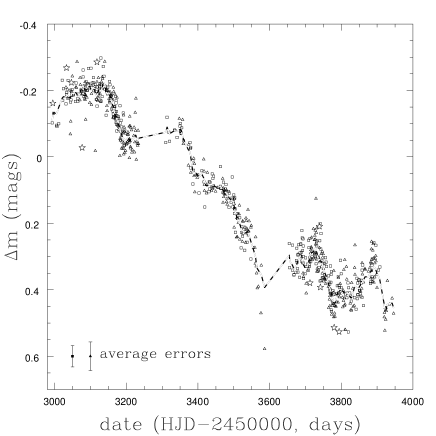
Figure 7: The overlapping A (squares) and B (triangles) light curves after shifting by the time delay and subtracting the estimated microlensing variability. The curve is the best fit $N_{src}=60$ source light curve model. There are three independent fits, one for each season, connected by a line through the seasonal gaps. The stars are the points that were masked in the time delay analysis. To minimize the confusion we are showing only the data with uncertainties smaller than 0.1 mag and include examples of their mean error bars in the lower left corner.

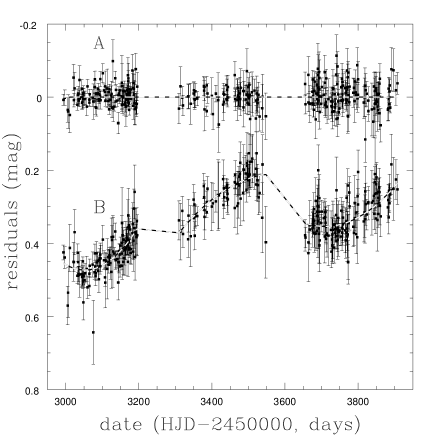
Figure 8: The inferred microlensing variability. We assigned the microlensing variability to image B, leaving the model for image A as a constant. This is an arbitrary choice that has no effect on the time delay – all we can really measure is the differential microlensing between the two images. The curves show the constant model used for A, the quadratic model ($N_{\mu}=3$) for B and only the data with uncertainties smaller than 0.1 mag. There are three independent fits, one for each season, connected by a line through the seasonal gaps.

3.4 Constraints on the long delays

The model predictions for the long time delays between the close image pair A and B and the fainter images C and D are very uncertain. For example, Oguri et al. (2004) found an approximate scaling relation of $\Delta t_{\mathrm{CD}}/\Delta t_{\mathrm{BA}}=143\pm 16$ for their models, which would imply a 15 year C/D time delay given our results for the A/B time delay. On the other hand, Williams & Saha (2004) found delay estimates of order $\Delta t_{\mathrm{CB}}~{}\approx~{}400$ days and $\Delta t_{\mathrm{AD}}~{}\approx~{}600$ days, albeit with a large scatter (about $\pm 200$ days). As we will discuss in §4, these studies use simplified mass models that are of only limited use for calibrating our expectations.

Empirically, with our 1000 day time span for the light curves we can test for image C and D delays of $\pm 1000$ days. We did so by matching the C or D light curve to the combined A/B light curves using the polynomial method. Since the overall behavior of the A and B light curves during the first and second season is mainly decreasing or flat while the light curve of image C shows an increase in the first season (Fig. 3), the time delay between C and B (with C leading) must be larger than 560 days. Assuming C is leading, there is a minimum near $681\pm 15$ days which corresponds to aligning the minimum observed in the first season for C with that observed in the last season for A/B. Due to the very different shapes of the light curves of images A/B and D there is no obvious solution over the whole observed time span. The only possibility would be to match the plateau in the third-year data of image D with the initial portions of the first-year data of images A/B, but there is no good candidate minimum in the goodness of fit. Therefore, we conclude that the time delay between A and D is larger than 800 days.

4 Models and Interpretation

We modeled the system using lensmodel (Keeton 2001) and the same component positions as were used by Kawanao & Oguri (2006) and Inada et al. (2006). We fitted all five quasar images assuming astrometric minimum uncertainties of $0\farcs 003$ and 20% flux uncertainties that are comparable to the observed amount of microlensing. We used the accurate but slow image plane fitting method, and the Hubble constant was fixed at $H_{0}=72$ km s^-1 Mpc^-1. The brightest cluster galaxy was modeled as an ellipsoidal de Vaucouleurs model with a major axis effective radius of $R_{e}=4\farcs 5$, an ellipticity of $0.18\pm 02$ and a major axis position angle of $-12^{\circ}\pm 5^{\circ}$ based on fits to the CASTLES project’s Hubble Space Telescope (HST) NICMOS H-band image of the system. The cluster halo was modeled as an ellipsoidal NFW model with a break radius of $r_{s}=40\farcs 0$ based on the mass model for the X-ray emission by Ota et al. (2006). We assumed priors on the ellipticity of the halo of $0.18\pm 0.05$, no prior on its major axis position angle, and a prior on the external shear of $\gamma=0.05\pm 0.05$. We also imposed hard limits on the ellipticity and position angle of the central galaxy ($0.15$ to $0.25$ and $-22^{\circ}$ to $-2^{\circ}$), the galaxy position ($\pm 0\farcs 3$ in each coordinate), the ellipticity of the halo ($0.0$ to $0.5$), the position of the halo ($\pm 3\farcs 0$ relative to the central galaxy) and the shear ($0\leq\gamma\leq 0.25$).

We first ran a model sequence based on simply adding a halo to the central galaxy. We started by fitting a de Vaucouleurs model with no halo to get the mass scale needed for the central galaxy in the absence of a halo. Then we fitted a series of models with the mass of the central galaxy fixed to a fraction $0\leq f\leq 1$ of its value in the no halo model. We ran the series both with and without the putative fifth quasar image. In general, the results are poor. The best fits to the image positions are obtained for $f\simeq 0.1$. The time delays for these models strongly disagree with our measurement in the sense that the model A–B delays are too short ($\sim 15$ days for $f=0.1$). Producing a longer delay requires a model with a lower surface density near the images, since the time delays of these simple models are roughly proportional to $1-\langle\kappa\rangle$ where $\langle\kappa\rangle$ is the mean surface density in the annulus between the images (see Kochanek 2002). However, the models with $f\simeq 0.7$ and a low surface density which fit the delay correctly, fit the images poorly and have ellipticities for both the galaxy and the halo that are driven to their maximum permitted values because a side effect of lowering the surface density is to increase the required ellipticity (see Kochanek 2005). That these simple models fit our delay measurement poorly is not surprising since the published results based on these simple model classes never produced a delay as long as our measured value.

The fundamental problem with this model, and all the preceding models of Oguri et al. (2004), Williams & Saha (2004), and Kawano & Oguri (2006), is that they neglect or poorly represent the substructure in the potential due to the presence of the other cluster galaxies. Many of these galaxies have deflection scales that are enormous compared to the astrometric uncertainties in the image positions, and as we painfully learned over 20 years of modeling Q0957 +561, astrometric uncertainties can be imposed to no greater accuracy than the deflection scales of the most massive neglected components of the mass distribution (see Keeton et al. 2000, Kochanek 2005). In short, the model sequence we just considered, as well as all published models of this system, was virtually guaranteed to be quantitatively incorrect.

At a minimum, the model needs to include galaxies whose deflections cannot be trivially mimicked by rescaling the mass of the central galaxy and modifying the external shear. We used Sextractor (Bertin & Arnouts 1996) to determine the positions and fluxes of the galaxies in the CASTLES HST/ACS I-band image of the cluster. We assumed the galaxies had critical radii that scaled with the square root of their flux (i.e. SIS models obeying a Tully-Fisher relation), and added the 11 most important galaxies within $20\farcs 0$ of the main lens galaxy as circular pseudo-Jaffe models ($\rho\propto r^{-2}[r^{2}+a^{2}]^{-1}$) with a break radius of $a=1\farcs 0$. We required that they have mass scales (Einstein radii) in the range $0\farcs 05\leq b\leq 2\farcs 0$ and kept their positions fixed. We did not attempt to force a correlation between flux and Einstein radius as the scatter in the relation is fairly large (Rusin et al. 2003). Figure 9 shows the positions of these galaxies relative to the image positions and the cluster center. We then ran the same sequence of models for the central galaxy and halo. These models have no difficulty fitting both the time delay and the image positions with reasonable parameters and a dark-matter dominated cluster model ($f\simeq 0.1$). Given the sensitivity of the A/B delay to substructure, it is probably premature to use the time delays as a strong constraint on the structure of the cluster. Reasonable models predict B/C delays of order 450 to 1000 days, suggesting that the roughly 680 day solution in §3.4 may well be correct, and that the A/D delays are of order 5–7 years. These longer delays should be much less sensitive to the perturbations from galaxies and will provide a better basis for studying the cluster.

Figure 9: A lens model generally consistent with the data. The open squares show the positions of the 5 lensed images A–E. The solid lines show the critical curves of the lens model, whose considerable, but realistic, complexity is due to the presence of the main lens galaxy (filled square), an offset halo (filled triangle), and 11 smaller galaxies (large crosses). The model fits the time delays and the image positions nearly perfectly.

Figure 9 shows the critical line structure of an illustrative model. Since the best models lead to B/C delays quite close to the value of $681$ days found by matching the minimum in the first season for C with those in the last season for A/B, we added it as a constraint. The model fits the image positions and the two time delays well but not perfectly, and there is a modest ($\chi^{2}=11.5$) 0$\farcs$1 westward offset of the lens galaxy suggesting that there are some remaining issues for fitting image E. In this model, the D image time delay relative to A and B is approximately 5.7 years and the central galaxy has 10% of the mass it would require in the absence of the dark matter halo. The Einstein radii of the smaller galaxies range from 0$\farcs$05 to 1$\farcs$4, which are plausible mass scales. The offset between the main lens galaxy and the dark matter halo found in earlier models still seems to be required. It is not our present intent to conduct a full model survey, but to emphasize the need for realistic models.

5 Summary and Conclusions

We have measured the A/B time delay of SDSS J1004+4112 to be $(38.4\pm 2.0)$ days ($\Delta\chi^{2}=4$), which fixes the overall time ordering of the images to be C-B-A-D-E. While this is the time ordering predicted in published models (Oguri et al. 2004, Williams & Saha 2004, Kawano & Oguri 2006) it is significantly longer than the delays predicted by these models. The cause of the discrepancy is that the previously published models overly simplified the mass distribution by neglecting the deflections generated by the cluster member galaxies.

Models including the eleven most important galaxies can simultaneously fit the A–E image positions and the measured A/B time delay with reasonable parameter values. Modelers of this system need to remember the lesson of Q0957+561 – model constraints that are applied more tightly than the deflection scale of the most massive, neglected components of the lens lead to incorrect results (Keeton et al. 2000). We note that Sharon et al. (2005) also needed to include some of the member galaxies in order to model the higher redshift lensed arcs, but made no predictions for the time delay.

Fortunately, the A/B delay should be the most sensitive of the delays to the effects of cluster galaxies because it is a merging image pair. The longer delays for the C and D images relative to A and B should be less affected by substructure, so their measurement should provide constraints on the cluster halo properties that are less sensitive to the member galaxies. At present we cannot claim a measurement of these longer delays. A lower bound on the delay $\Delta t_{\mathrm{AD}}>800$ days is consistent with our models, which predict delays of 5–7 years for this image pair. The shorter C/B delay is at least $\Delta t_{\mathrm{CB}}>560$ days but there is a possible delay of $\Delta t_{\mathrm{CB}}\simeq 680\pm 15$ days that should be confirmed or rejected during the next observing seasons and is consistent with our models.

We have also clearly detected microlensing variability in the A/B images, with changes of order $0.15$ mag in the A/B flux ratio over the course of the three observing seasons. This result provides strong evidence that the differential changes in the A/B emission line profiles are also due to microlensing (Richards et al. 2004, Lamer et al. 2006, Gómez-Álvarez et al. 2006) rather than variable absorption in the source (Green 2006). The microlensing time scales in SDSS J1004+4112 should be relatively shorter than in most single galaxy lenses because the internal velocities of the cluster are about 3 times higher than those of a galaxy. While the flux ratio changes in the optical continuum are modest, we would expect to find significantly larger effects at shorter wavelengths where the source size should be more compact. There is already some evidence for this from the X-ray flux ratios measured by Ota et al. (2006) and Lamer et al. (2006). A campaign to monitor this system in X-rays would both allow us to study the size of the X-ray emission region and provide the added data on the emission from the cluster needed to provide a precision comparison of the mass distributions estimated using X-ray data and lens models. Such careful tests will be essential if measurements of the increase of the Einstein radius of the cluster with source redshift based on the surrounding multiply imaged arcs are to be used as a new test of the cosmological model as proposed by Soucail et al. (2004) and Sharon et al. (2005).

Table 1: Light Curves for SDSS J1004+4112 A&B

HJD	$\chi^{2}/N_{dof}$	Image A	Image B	Observatory	Detector
2993.523	0.93	3.185 $\pm$ 0.015	3.533 $\pm$ 0.020	FLWO	4Shooter
2994.960	2.20	(3.127 $\pm$ 0.007)	(3.475 $\pm$ 0.007)	MDM	8K
2996.599	1.82	3.127 $\pm$ 0.048	3.667 $\pm$ 0.079	Wise	Tektronix
2997.344	0.76	3.157 $\pm$ 0.021	3.541 $\pm$ 0.029	FLWO	4Shooter
2997.598	2.42	3.107 $\pm$ 0.041	3.602 $\pm$ 0.065	Wise	Tektronix
2998.560	52.09	3.805 $\pm$ 0.039	5.411 $\pm$ 0.160	Wise	Tektronix
3001.632	135.90	4.045 $\pm$ 0.036	5.658 $\pm$ 0.146	Wise	Tektronix
3004.596	53.91	3.678 $\pm$ 0.031	4.765 $\pm$ 0.080	Wise	Tektronix
3005.538	1.33	3.193 $\pm$ 0.029	3.681 $\pm$ 0.045	Wise	Tektronix
3006.519	3.71	3.197 $\pm$ 0.024	3.643 $\pm$ 0.035	Wise	Tektronix
3011.405	0.75	3.188 $\pm$ 0.047	3.509 $\pm$ 0.062	FLWO	4Shooter
3021.543	3.94	3.057 $\pm$ 0.018	3.546 $\pm$ 0.026	Wise	Tektronix
3022.606	1.53	3.118 $\pm$ 0.015	3.548 $\pm$ 0.021	FLWO	4Shooter
3024.524	0.78	3.083 $\pm$ 0.043	3.471 $\pm$ 0.060	Wise	Tektronix
3031.920	1.48	3.128 $\pm$ 0.013	3.588 $\pm$ 0.018	FLWO	4Shooter
3032.920	2.02	3.101 $\pm$ 0.013	3.521 $\pm$ 0.017	FLWO	4Shooter
3033.913	2.53	3.094 $\pm$ 0.013	3.542 $\pm$ 0.017	FLWO	4Shooter
3034.916	1.03	3.107 $\pm$ 0.014	3.571 $\pm$ 0.020	FLWO	4Shooter
3035.382	3.21	3.199 $\pm$ 0.056	3.745 $\pm$ 0.097	Wise	TAVAS
3035.909	1.71	3.111 $\pm$ 0.013	3.570 $\pm$ 0.019	FLWO	4Shooter
3037.742	0.73	3.058 $\pm$ 0.039	3.562 $\pm$ 0.060	FLWO	4Shooter
3038.720	1.48	3.111 $\pm$ 0.018	(3.732 $\pm$ 0.031)	MDM	Templeton
3043.854	0.51	3.087 $\pm$ 0.025	3.564 $\pm$ 0.037	FLWO	4Shooter
3044.885	1.39	3.123 $\pm$ 0.015	3.574 $\pm$ 0.022	FLWO	4Shooter
3045.862	2.69	3.116 $\pm$ 0.011	3.573 $\pm$ 0.016	FLWO	4Shooter
3046.908	1.52	3.091 $\pm$ 0.012	3.589 $\pm$ 0.017	FLWO	4Shooter
3046.949	0.99	(3.064 $\pm$ 0.011)	3.536 $\pm$ 0.012	APO	SPICam
3047.866	3.72	3.103 $\pm$ 0.009	3.574 $\pm$ 0.013	FLWO	4Shooter
3048.453	1.13	3.096 $\pm$ 0.028	3.649 $\pm$ 0.045	Wise	Tektronix
3048.885	1.38	3.085 $\pm$ 0.011	3.577 $\pm$ 0.016	FLWO	4Shooter
3051.850	2.56	3.102 $\pm$ 0.009	3.582 $\pm$ 0.013	FLWO	4Shooter
3052.425	1.76	3.073 $\pm$ 0.045	3.756 $\pm$ 0.081	Wise	Tektronix
3052.869	2.82	3.100 $\pm$ 0.011	3.560 $\pm$ 0.016	FLWO	4Shooter
3053.605	3.49	(3.450 $\pm$ 0.035)	(4.165 $\pm$ 0.065)	Wise	Tektronix
3056.349	9.58	1.568 $\pm$ 0.299	(0.760 $\pm$ 0.151)	Wise	TAVAS
3057.341	2.12	2.896 $\pm$ 0.061	3.672 $\pm$ 0.128	Wise	TAVAS
3057.795	2.78	3.121 $\pm$ 0.015	3.543 $\pm$ 0.021	FLWO	4Shooter
3058.362	1.04	2.949 $\pm$ 0.116	3.554 $\pm$ 0.195	Wise	TAVAS
3059.347	3.96	3.010 $\pm$ 0.069	3.368 $\pm$ 0.100	Wise	TAVAS
3059.856	0.67	3.066 $\pm$ 0.019	3.598 $\pm$ 0.030	FLWO	4Shooter
3060.353	2.51	2.894 $\pm$ 0.065	3.493 $\pm$ 0.122	Wise	TAVAS
3061.365	3.55	3.138 $\pm$ 0.048	3.506 $\pm$ 0.070	Wise	TAVAS
3062.396	4.27	3.154 $\pm$ 0.036	3.563 $\pm$ 0.052	Wise	TAVAS
3064.468	35.89	3.823 $\pm$ 0.054	5.480 $\pm$ 0.226	Wise	Tektronix
3064.773	1.01	3.112 $\pm$ 0.017	3.603 $\pm$ 0.026	FLWO	4Shooter
3064.884	1.41	3.121 $\pm$ 0.007	3.570 $\pm$ 0.008	MDM	Echelle
3065.480	12.90	3.191 $\pm$ 0.057	3.958 $\pm$ 0.112	Wise	Tektronix
3065.805	2.91	3.099 $\pm$ 0.008	3.547 $\pm$ 0.011	FLWO	4Shooter
3073.862	0.59	3.086 $\pm$ 0.023	3.547 $\pm$ 0.034	FLWO	4Shooter
3075.464	1.03	3.091 $\pm$ 0.047	3.740 $\pm$ 0.083	Wise	Tektronix
3078.837	1.12	3.077 $\pm$ 0.012	3.584 $\pm$ 0.018	FLWO	4Shooter
3079.832	1.77	3.048 $\pm$ 0.013	3.531 $\pm$ 0.019	FLWO	4Shooter
3079.848	11.73	3.026 $\pm$ 0.007	(3.471 $\pm$ 0.007)	MDM	8K
3080.822	1.01	3.077 $\pm$ 0.013	3.566 $\pm$ 0.019	FLWO	4Shooter
3081.327	2.06	3.005 $\pm$ 0.062	3.454 $\pm$ 0.099	Wise	TAVAS
3081.789	3.07	3.107 $\pm$ 0.011	3.587 $\pm$ 0.015	FLWO	4Shooter
3082.785	1.69	3.072 $\pm$ 0.011	3.576 $\pm$ 0.016	FLWO	4Shooter
3083.934	1.01	3.113 $\pm$ 0.022	3.517 $\pm$ 0.031	FLWO	4Shooter
3085.793	1.45	3.087 $\pm$ 0.011	3.539 $\pm$ 0.015	FLWO	4Shooter
3087.662	3.09	3.012 $\pm$ 0.061	3.498 $\pm$ 0.061	WIYN	WTTM
3087.707	2.40	3.077 $\pm$ 0.011	3.534 $\pm$ 0.016	FLWO	4Shooter
3088.734	2.01	3.063 $\pm$ 0.011	3.563 $\pm$ 0.016	FLWO	4Shooter
3090.735	0.63	3.088 $\pm$ 0.024	3.587 $\pm$ 0.036	FLWO	4Shooter
3091.772	0.97	3.080 $\pm$ 0.014	3.534 $\pm$ 0.020	FLWO	4Shooter
3092.821	0.65	3.069 $\pm$ 0.017	3.527 $\pm$ 0.025	FLWO	4Shooter
3093.790	0.72	3.068 $\pm$ 0.014	3.546 $\pm$ 0.021	FLWO	4Shooter
3094.718	0.80	3.022 $\pm$ 0.020	3.510 $\pm$ 0.031	FLWO	4Shooter
3095.819	0.67	3.080 $\pm$ 0.024	3.516 $\pm$ 0.035	FLWO	4Shooter
3100.412	0.36	3.085 $\pm$ 0.093	3.529 $\pm$ 0.137	Wise	Tektronix
3101.657	0.42	3.021 $\pm$ 0.026	3.461 $\pm$ 0.038	FLWO	4Shooter
3104.747	0.99	3.066 $\pm$ 0.017	3.534 $\pm$ 0.025	FLWO	4Shooter
3107.686	1.31	3.027 $\pm$ 0.755	3.486 $\pm$ 0.755	WIYN	WTTM
3107.694	0.66	3.065 $\pm$ 0.015	3.591 $\pm$ 0.024	FLWO	4Shooter
3108.285	1.84	3.050 $\pm$ 0.031	3.606 $\pm$ 0.049	Wise	Tektronix
3108.729	1.64	3.089 $\pm$ 0.012	3.544 $\pm$ 0.016	FLWO	4Shooter
3111.688	1.61	3.083 $\pm$ 0.013	3.546 $\pm$ 0.018	FLWO	4Shooter
3113.335	0.89	3.071 $\pm$ 0.051	3.566 $\pm$ 0.080	Wise	Tektronix
3116.725	1.37	3.115 $\pm$ 0.013	3.542 $\pm$ 0.017	FLWO	4Shooter
3117.746	1.36	3.091 $\pm$ 0.014	3.567 $\pm$ 0.020	FLWO	4Shooter
3118.764	0.82	3.135 $\pm$ 0.014	3.552 $\pm$ 0.019	FLWO	4Shooter
3119.731	0.76	3.077 $\pm$ 0.014	3.551 $\pm$ 0.020	FLWO	4Shooter
3120.730	0.70	3.102 $\pm$ 0.015	3.561 $\pm$ 0.022	FLWO	4Shooter
3122.786	0.55	3.096 $\pm$ 0.028	3.583 $\pm$ 0.043	FLWO	4Shooter
3124.718	0.78	3.083 $\pm$ 0.027	3.614 $\pm$ 0.044	FLWO	4Shooter
3125.737	0.52	3.077 $\pm$ 0.034	3.523 $\pm$ 0.051	FLWO	4Shooter
3126.717	0.58	3.117 $\pm$ 0.027	3.534 $\pm$ 0.039	FLWO	4Shooter
3129.240	0.72	2.991 $\pm$ 0.057	3.577 $\pm$ 0.094	Wise	Tektronix
3129.812	0.58	3.120 $\pm$ 0.035	3.539 $\pm$ 0.051	FLWO	4Shooter
3132.749	2.09	3.106 $\pm$ 0.008	3.596 $\pm$ 0.012	FLWO	4Shooter
3135.717	7.04	3.016 $\pm$ 0.007	3.544 $\pm$ 0.009	MDM	8K
3136.659	1.65	3.077 $\pm$ 0.013	3.625 $\pm$ 0.019	FLWO	4Shooter
3137.719	1.15	3.045 $\pm$ 0.013	3.627 $\pm$ 0.021	FLWO	4Shooter
3140.640	1.58	3.084 $\pm$ 0.013	3.636 $\pm$ 0.019	FLWO	4Shooter
3143.790	0.63	3.162 $\pm$ 0.029	3.712 $\pm$ 0.047	FLWO	4Shooter
3144.677	1.61	3.089 $\pm$ 0.012	3.659 $\pm$ 0.019	FLWO	4Shooter
3145.711	1.55	3.087 $\pm$ 0.014	3.663 $\pm$ 0.023	FLWO	4Shooter
3146.745	0.84	3.093 $\pm$ 0.013	3.636 $\pm$ 0.020	FLWO	4Shooter
3147.648	1.42	3.098 $\pm$ 0.015	3.648 $\pm$ 0.023	FLWO	4Shooter
3148.653	1.34	3.078 $\pm$ 0.015	3.684 $\pm$ 0.025	FLWO	4Shooter
3149.733	1.37	3.094 $\pm$ 0.013	3.631 $\pm$ 0.020	FLWO	4Shooter
3153.660	1.40	3.060 $\pm$ 0.061	3.631 $\pm$ 0.061	WIYN	WTTM
3153.692	0.86	3.120 $\pm$ 0.019	3.661 $\pm$ 0.030	FLWO	4Shooter
3154.272	0.33	3.071 $\pm$ 0.059	3.578 $\pm$ 0.093	Wise	Tektronix
3154.673	0.66	3.125 $\pm$ 0.023	3.695 $\pm$ 0.037	FLWO	4Shooter
3155.673	0.62	3.106 $\pm$ 0.024	3.613 $\pm$ 0.037	FLWO	4Shooter
3156.646	0.72	3.113 $\pm$ 0.020	3.625 $\pm$ 0.031	FLWO	4Shooter
3157.670	0.67	3.100 $\pm$ 0.021	3.688 $\pm$ 0.034	FLWO	4Shooter
3158.660	1.04	3.105 $\pm$ 0.017	3.628 $\pm$ 0.026	FLWO	4Shooter
3159.643	0.57	3.145 $\pm$ 0.029	3.679 $\pm$ 0.046	FLWO	4Shooter
3161.736	2.88	3.116 $\pm$ 0.016	3.658 $\pm$ 0.024	MDM	Templeton
3162.658	2.80	3.150 $\pm$ 0.008	3.653 $\pm$ 0.010	MDM	Templeton
3163.650	4.10	3.159 $\pm$ 0.010	3.653 $\pm$ 0.013	MDM	Templeton
3164.651	28.62	3.168 $\pm$ 0.010	3.646 $\pm$ 0.014	MDM	Templeton
3165.656	11.23	3.171 $\pm$ 0.008	3.623 $\pm$ 0.011	MDM	Templeton
3166.650	3.74	3.142 $\pm$ 0.009	3.615 $\pm$ 0.012	MDM	Templeton
3167.665	8.23	3.136 $\pm$ 0.006	3.621 $\pm$ 0.006	MDM	Templeton
3168.663	17.04	3.152 $\pm$ 0.006	3.636 $\pm$ 0.007	MDM	Templeton
3169.662	6.01	3.171 $\pm$ 0.006	3.635 $\pm$ 0.007	MDM	Templeton
3169.674	1.08	3.164 $\pm$ 0.015	3.642 $\pm$ 0.021	FLWO	4Shooter
3170.259	0.28	3.106 $\pm$ 0.047	3.593 $\pm$ 0.073	Wise	Tektronix
3170.667	0.71	3.169 $\pm$ 0.011	3.630 $\pm$ 0.016	MDM	Templeton
3170.673	0.60	3.174 $\pm$ 0.025	3.687 $\pm$ 0.039	FLWO	4Shooter
3171.271	0.33	3.126 $\pm$ 0.048	3.562 $\pm$ 0.072	Wise	Tektronix
3171.661	1.78	3.185 $\pm$ 0.007	3.634 $\pm$ 0.009	MDM	Templeton
3171.666	1.22	3.119 $\pm$ 0.019	3.635 $\pm$ 0.030	FLWO	4Shooter
3172.664	1.68	3.190 $\pm$ 0.007	3.634 $\pm$ 0.008	MDM	Templeton
3172.668	0.73	3.151 $\pm$ 0.016	3.589 $\pm$ 0.022	FLWO	4Shooter
3173.658	0.68	3.164 $\pm$ 0.017	3.650 $\pm$ 0.025	FLWO	4Shooter
3173.659	4.56	3.210 $\pm$ 0.007	3.654 $\pm$ 0.008	MDM	Templeton
3174.664	0.71	3.173 $\pm$ 0.016	3.591 $\pm$ 0.023	FLWO	4Shooter
3176.666	1.00	3.172 $\pm$ 0.016	3.596 $\pm$ 0.022	FLWO	4Shooter
3177.675	1.14	3.167 $\pm$ 0.018	3.661 $\pm$ 0.027	FLWO	4Shooter
3178.675	0.63	3.197 $\pm$ 0.027	3.652 $\pm$ 0.040	FLWO	4Shooter
3182.654	0.67	3.134 $\pm$ 0.043	3.604 $\pm$ 0.067	FLWO	4Shooter
3183.653	0.66	3.186 $\pm$ 0.040	3.578 $\pm$ 0.057	FLWO	4Shooter
3184.653	0.64	3.237 $\pm$ 0.036	3.651 $\pm$ 0.052	FLWO	4Shooter
3185.652	0.60	3.178 $\pm$ 0.034	3.619 $\pm$ 0.050	FLWO	4Shooter
3186.651	0.57	3.198 $\pm$ 0.039	3.529 $\pm$ 0.052	FLWO	4Shooter
3187.651	0.56	3.217 $\pm$ 0.039	3.582 $\pm$ 0.054	FLWO	4Shooter
3188.653	0.70	3.243 $\pm$ 0.057	3.483 $\pm$ 0.071	FLWO	4Shooter
3189.656	0.66	3.262 $\pm$ 0.042	3.666 $\pm$ 0.061	FLWO	4Shooter
3191.652	0.72	3.156 $\pm$ 0.042	3.608 $\pm$ 0.063	FLWO	4Shooter
3192.660	0.81	3.262 $\pm$ 0.020	3.613 $\pm$ 0.027	FLWO	4Shooter
3193.650	0.78	3.254 $\pm$ 0.034	3.618 $\pm$ 0.047	FLWO	4Shooter
3194.654	0.95	3.253 $\pm$ 0.027	3.571 $\pm$ 0.036	FLWO	4Shooter
3195.652	0.63	3.208 $\pm$ 0.038	3.610 $\pm$ 0.054	FLWO	4Shooter
3310.011	0.35	3.245 $\pm$ 0.041	3.544 $\pm$ 0.052	FLWO	Minicam
3314.010	0.27	3.169 $\pm$ 0.052	3.576 $\pm$ 0.075	FLWO	Minicam
3315.021	0.17	3.178 $\pm$ 0.119	3.782 $\pm$ 0.199	FLWO	Minicam
3318.964	0.80	3.214 $\pm$ 0.030	3.537 $\pm$ 0.039	FLWO	Minicam
3321.023	0.55	3.241 $\pm$ 0.027	3.607 $\pm$ 0.036	FLWO	Minicam
3335.040	0.60	3.207 $\pm$ 0.034	3.656 $\pm$ 0.049	FLWO	Minicam
3336.026	0.48	3.208 $\pm$ 0.032	3.592 $\pm$ 0.044	FLWO	Minicam
3341.993	0.38	3.230 $\pm$ 0.055	3.670 $\pm$ 0.080	FLWO	Minicam
3349.604	4.16	3.263 $\pm$ 0.065	3.669 $\pm$ 0.093	Wise	TAVAS
3350.012	0.42	3.196 $\pm$ 0.029	3.619 $\pm$ 0.040	FLWO	Minicam
3350.998	0.72	3.187 $\pm$ 0.023	3.671 $\pm$ 0.033	FLWO	Minicam
3352.044	0.55	3.212 $\pm$ 0.023	3.633 $\pm$ 0.032	FLWO	Minicam
3352.572	2.39	3.297 $\pm$ 0.059	3.776 $\pm$ 0.092	Wise	TAVAS
3353.038	0.90	3.217 $\pm$ 0.026	3.717 $\pm$ 0.038	FLWO	Minicam
3354.033	0.79	3.218 $\pm$ 0.023	3.664 $\pm$ 0.031	FLWO	Minicam
3354.920	0.89	3.200 $\pm$ 0.021	3.661 $\pm$ 0.030	FLWO	Minicam
3359.000	1.64	3.261 $\pm$ 0.047	3.876 $\pm$ 0.079	Wise	Tektronix
3359.920	1.24	3.239 $\pm$ 0.018	3.667 $\pm$ 0.023	FLWO	Minicam
3360.000	0.40	3.302 $\pm$ 0.093	3.631 $\pm$ 0.124	Wise	Tektronix
3377.879	0.71	3.245 $\pm$ 0.026	3.595 $\pm$ 0.034	FLWO	Minicam
3378.945	0.43	3.263 $\pm$ 0.027	3.630 $\pm$ 0.036	FLWO	Minicam
3379.878	0.42	3.260 $\pm$ 0.025	3.688 $\pm$ 0.035	FLWO	Minicam
3380.000	1.33	3.321 $\pm$ 0.050	3.669 $\pm$ 0.067	Wise	Tektronix
3380.606	2.78	3.415 $\pm$ 0.049	3.854 $\pm$ 0.075	Wise	TAVAS
3381.581	1.62	3.463 $\pm$ 0.154	3.993 $\pm$ 0.238	Wise	TAVAS
3384.554	2.65	3.312 $\pm$ 0.073	3.680 $\pm$ 0.101	Wise	TAVAS
3385.816	0.45	3.370 $\pm$ 0.014	3.690 $\pm$ 0.015	APO	SPICam
3385.951	0.63	3.300 $\pm$ 0.024	3.663 $\pm$ 0.031	FLWO	Minicam
3386.453	2.74	3.303 $\pm$ 0.079	3.653 $\pm$ 0.114	Wise	TAVAS
3387.527	2.92	3.321 $\pm$ 0.087	3.609 $\pm$ 0.109	Wise	TAVAS
3387.960	0.69	3.328 $\pm$ 0.027	3.626 $\pm$ 0.033	FLWO	Minicam
3399.018	0.30	3.341 $\pm$ 0.067	3.752 $\pm$ 0.096	FLWO	Minicam
3399.714	0.25	3.342 $\pm$ 0.049	3.671 $\pm$ 0.064	FLWO	Minicam
3402.990	0.27	3.397 $\pm$ 0.041	3.663 $\pm$ 0.052	FLWO	Minicam
3403.412	1.99	3.317 $\pm$ 0.063	3.826 $\pm$ 0.101	Wise	TAVAS
3406.322	1.32	3.330 $\pm$ 0.099	3.742 $\pm$ 0.146	Wise	TAVAS
3408.375	1.96	3.408 $\pm$ 0.067	3.688 $\pm$ 0.086	Wise	TAVAS
3410.806	0.78	3.330 $\pm$ 0.023	3.664 $\pm$ 0.029	FLWO	Minicam
3411.452	2.81	(2.988 $\pm$ 0.065)	3.489 $\pm$ 0.107	Wise	TAVAS
3412.404	2.20	3.586 $\pm$ 0.092	3.777 $\pm$ 0.108	Wise	TAVAS
3416.000	0.63	3.531 $\pm$ 0.103	3.639 $\pm$ 0.113	Wise	Tektronix
3417.000	0.90	3.363 $\pm$ 0.072	3.648 $\pm$ 0.093	Wise	Tektronix
3419.000	0.51	3.439 $\pm$ 0.073	3.647 $\pm$ 0.088	Wise	Tektronix
3430.930	0.28	3.393 $\pm$ 0.043	3.611 $\pm$ 0.051	FLWO	Minicam
3431.738	0.59	3.362 $\pm$ 0.028	3.683 $\pm$ 0.036	FLWO	Minicam
3432.721	0.55	3.385 $\pm$ 0.028	3.639 $\pm$ 0.035	FLWO	Minicam
3433.740	0.93	3.364 $\pm$ 0.025	3.665 $\pm$ 0.031	FLWO	Minicam
3439.643	0.39	3.377 $\pm$ 0.013	3.643 $\pm$ 0.014	APO	SPICam
3439.719	0.71	3.339 $\pm$ 0.025	3.650 $\pm$ 0.032	FLWO	Minicam
3441.615	0.34	3.380 $\pm$ 0.014	3.639 $\pm$ 0.015	APO	SPICam
3441.797	0.60	3.353 $\pm$ 0.030	3.674 $\pm$ 0.038	FLWO	Minicam
3442.734	0.84	3.374 $\pm$ 0.026	3.664 $\pm$ 0.032	FLWO	Minicam
3443.748	1.17	3.346 $\pm$ 0.029	3.681 $\pm$ 0.038	FLWO	Minicam
3459.333	1.39	3.322 $\pm$ 0.068	3.780 $\pm$ 0.101	Wise	TAVAS
3462.836	0.31	3.317 $\pm$ 0.037	3.739 $\pm$ 0.052	FLWO	Minicam
3462.859	1.17	3.376 $\pm$ 0.013	3.669 $\pm$ 0.015	APO	SPICam
3463.722	0.55	3.384 $\pm$ 0.031	3.653 $\pm$ 0.038	FLWO	Minicam
3464.719	0.81	3.382 $\pm$ 0.023	3.684 $\pm$ 0.029	FLWO	Minicam
3466.251	1.65	3.515 $\pm$ 0.083	3.917 $\pm$ 0.119	Wise	TAVAS
3467.320	2.26	3.494 $\pm$ 0.063	3.793 $\pm$ 0.083	Wise	TAVAS
3468.291	1.45	3.318 $\pm$ 0.086	3.774 $\pm$ 0.130	Wise	TAVAS
3469.756	0.34	3.396 $\pm$ 0.055	3.766 $\pm$ 0.074	FLWO	Minicam
3470.713	0.47	3.364 $\pm$ 0.026	3.707 $\pm$ 0.033	FLWO	Minicam
3471.000	0.50	3.457 $\pm$ 0.085	3.746 $\pm$ 0.109	Wise	Tektronix
3471.763	0.32	3.386 $\pm$ 0.029	3.763 $\pm$ 0.039	FLWO	Minicam
3472.766	0.85	3.397 $\pm$ 0.025	3.709 $\pm$ 0.031	FLWO	Minicam
3473.744	1.38	3.393 $\pm$ 0.020	3.694 $\pm$ 0.024	FLWO	Minicam
3474.743	0.84	3.398 $\pm$ 0.022	3.719 $\pm$ 0.028	FLWO	Minicam
3476.739	0.42	3.385 $\pm$ 0.043	3.693 $\pm$ 0.056	FLWO	Minicam
3477.735	0.57	3.401 $\pm$ 0.045	3.666 $\pm$ 0.056	FLWO	Minicam
3478.690	0.39	3.371 $\pm$ 0.051	3.768 $\pm$ 0.071	FLWO	Minicam
3485.738	0.33	3.392 $\pm$ 0.054	3.772 $\pm$ 0.074	FLWO	Minicam
3486.707	0.30	3.439 $\pm$ 0.052	3.709 $\pm$ 0.066	FLWO	Minicam
3487.675	1.08	3.397 $\pm$ 0.025	3.711 $\pm$ 0.032	FLWO	Minicam
3489.000	0.87	3.384 $\pm$ 0.072	4.182 $\pm$ 0.145	Wise	Tektronix
3492.710	0.46	3.425 $\pm$ 0.038	3.725 $\pm$ 0.049	FLWO	Minicam
3494.722	0.78	3.412 $\pm$ 0.025	3.771 $\pm$ 0.033	FLWO	Minicam
3495.722	0.28	3.349 $\pm$ 0.059	3.697 $\pm$ 0.080	FLWO	Minicam
3496.694	0.42	3.415 $\pm$ 0.028	3.704 $\pm$ 0.035	FLWO	Minicam
3497.720	0.43	3.439 $\pm$ 0.031	3.727 $\pm$ 0.039	FLWO	Minicam
3498.691	0.58	3.422 $\pm$ 0.026	3.732 $\pm$ 0.033	FLWO	Minicam
3499.695	0.73	3.402 $\pm$ 0.025	3.742 $\pm$ 0.032	FLWO	Minicam
3500.244	1.14	3.483 $\pm$ 0.108	3.678 $\pm$ 0.125	Wise	TAVAS
3501.245	1.28	3.415 $\pm$ 0.082	3.630 $\pm$ 0.100	Wise	TAVAS
3501.708	0.66	3.443 $\pm$ 0.044	3.670 $\pm$ 0.053	FLWO	Minicam
3501.817	0.21	3.458 $\pm$ 0.020	3.735 $\pm$ 0.024	APO	SPICam
3502.701	0.37	3.411 $\pm$ 0.033	3.746 $\pm$ 0.043	FLWO	Minicam
3503.666	0.74	3.444 $\pm$ 0.028	3.734 $\pm$ 0.035	FLWO	Minicam
3504.687	0.24	3.515 $\pm$ 0.068	3.702 $\pm$ 0.073	FLWO	Minicam
3509.698	0.31	3.459 $\pm$ 0.054	3.720 $\pm$ 0.068	FLWO	Minicam
3510.674	0.60	3.472 $\pm$ 0.052	3.715 $\pm$ 0.064	FLWO	Minicam
3516.680	0.53	3.471 $\pm$ 0.031	3.780 $\pm$ 0.040	FLWO	Minicam
3520.686	0.65	3.562 $\pm$ 0.035	3.778 $\pm$ 0.042	FLWO	Minicam
3521.691	0.51	3.515 $\pm$ 0.034	3.825 $\pm$ 0.044	FLWO	Minicam
3522.646	0.39	3.498 $\pm$ 0.047	3.746 $\pm$ 0.057	FLWO	Minicam
3524.667	0.63	3.527 $\pm$ 0.034	3.833 $\pm$ 0.043	FLWO	Minicam
3525.673	0.45	3.518 $\pm$ 0.034	3.854 $\pm$ 0.044	FLWO	Minicam
3527.651	0.70	3.507 $\pm$ 0.034	3.898 $\pm$ 0.047	FLWO	Minicam
3530.650	0.40	3.569 $\pm$ 0.039	3.893 $\pm$ 0.051	FLWO	Minicam
3536.660	0.29	3.547 $\pm$ 0.072	3.883 $\pm$ 0.096	FLWO	Minicam
3537.661	0.31	3.545 $\pm$ 0.064	3.971 $\pm$ 0.092	FLWO	Minicam
3538.652	0.43	3.514 $\pm$ 0.060	3.827 $\pm$ 0.078	FLWO	Minicam
3541.654	0.28	3.425 $\pm$ 0.117	3.984 $\pm$ 0.189	FLWO	Minicam
3547.650	0.30	3.595 $\pm$ 0.062	4.078 $\pm$ 0.094	FLWO	Minicam
3549.651	0.30	3.646 $\pm$ 0.084	4.040 $\pm$ 0.118	FLWO	Minicam
3655.027	3.46	3.548 $\pm$ 0.017	3.983 $\pm$ 0.023	MDM	RETROCAM
3656.000	5.00	3.621 $\pm$ 0.012	3.995 $\pm$ 0.012	MDM	RETROCAM
3664.001	1.09	3.553 $\pm$ 0.047	4.046 $\pm$ 0.072	FLWO	Keplercam
3664.001	4.27	3.629 $\pm$ 0.012	4.017 $\pm$ 0.014	MDM	RETROCAM
3667.967	0.59	3.643 $\pm$ 0.049	3.967 $\pm$ 0.065	FLWO	Keplercam
3668.006	3.51	3.643 $\pm$ 0.017	3.979 $\pm$ 0.021	MDM	RETROCAM
3673.899	0.49	3.635 $\pm$ 0.015	3.938 $\pm$ 0.017	APO	SPICam
3674.990	0.61	3.600 $\pm$ 0.038	3.942 $\pm$ 0.050	FLWO	Keplercam
3676.001	1.02	3.563 $\pm$ 0.025	3.928 $\pm$ 0.033	FLWO	Keplercam
3676.969	0.29	3.473 $\pm$ 0.088	3.710 $\pm$ 0.108	FLWO	Keplercam
3677.013	2.75	3.605 $\pm$ 0.015	3.919 $\pm$ 0.018	MDM	RETROCAM
3677.995	9.20	3.624 $\pm$ 0.011	3.911 $\pm$ 0.012	MDM	RETROCAM
3678.997	2.98	3.635 $\pm$ 0.012	3.914 $\pm$ 0.012	MDM	RETROCAM
3679.013	1.03	3.583 $\pm$ 0.034	3.881 $\pm$ 0.043	FLWO	Keplercam
3679.995	0.60	3.581 $\pm$ 0.038	3.947 $\pm$ 0.051	FLWO	Keplercam
3681.004	1.26	3.553 $\pm$ 0.024	3.949 $\pm$ 0.032	FLWO	Keplercam
3684.012	0.55	3.650 $\pm$ 0.052	3.856 $\pm$ 0.061	FLWO	Keplercam
3685.017	0.70	3.577 $\pm$ 0.033	3.944 $\pm$ 0.045	FLWO	Keplercam
3686.564	4.61	3.476 $\pm$ 0.066	3.829 $\pm$ 0.094	Wise	TAVAS
3686.892	1.46	3.550 $\pm$ 0.026	3.891 $\pm$ 0.035	Palomar	SITe
3687.024	0.89	3.551 $\pm$ 0.035	3.931 $\pm$ 0.048	FLWO	Keplercam
3688.016	1.28	3.589 $\pm$ 0.029	3.877 $\pm$ 0.037	FLWO	Keplercam
3688.929	1.86	3.602 $\pm$ 0.017	3.889 $\pm$ 0.020	MDM	RETROCAM
3689.034	0.54	3.575 $\pm$ 0.038	3.862 $\pm$ 0.048	FLWO	Keplercam
3690.002	0.43	3.510 $\pm$ 0.067	3.904 $\pm$ 0.095	FLWO	Keplercam
3691.019	0.56	3.532 $\pm$ 0.054	3.767 $\pm$ 0.067	FLWO	Keplercam
3691.898	1.70	3.570 $\pm$ 0.031	3.929 $\pm$ 0.042	Palomar	SITe
3692.018	0.40	3.607 $\pm$ 0.056	3.869 $\pm$ 0.070	FLWO	Keplercam
3693.022	0.38	3.535 $\pm$ 0.054	3.949 $\pm$ 0.077	FLWO	Keplercam
3693.865	0.59	3.588 $\pm$ 0.049	3.856 $\pm$ 0.062	Palomar	SITe
3693.927	0.28	3.607 $\pm$ 0.023	3.894 $\pm$ 0.028	APO	SPICam
3694.012	0.61	3.557 $\pm$ 0.048	3.986 $\pm$ 0.069	FLWO	Keplercam
3694.862	0.77	3.654 $\pm$ 0.046	3.977 $\pm$ 0.061	Palomar	SITe
3698.919	3.60	3.640 $\pm$ 0.012	3.945 $\pm$ 0.013	MDM	RETROCAM
3700.601	0.69	-0.13 $\pm$ 1.048	(-0.51 $\pm$ 0.926)	Wise	TAVAS
3700.927	1.32	3.592 $\pm$ 0.021	3.915 $\pm$ 0.027	FLWO	Keplercam
3700.997	1.99	3.618 $\pm$ 0.012	(3.851 $\pm$ 0.013)	MDM	RETROCAM
3701.581	0.87	3.002 $\pm$ 0.238	(3.054 $\pm$ 0.238)	Wise	TAVAS
3702.560	2.57	3.456 $\pm$ 0.104	3.595 $\pm$ 0.115	Wise	TAVAS
3706.012	3.42	3.611 $\pm$ 0.019	3.934 $\pm$ 0.024	FLWO	Keplercam
3707.581	3.31	3.480 $\pm$ 0.067	4.099 $\pm$ 0.120	Wise	TAVAS
3708.849	0.45	3.539 $\pm$ 0.045	3.992 $\pm$ 0.070	Palomar	SITe
3708.984	0.99	3.629 $\pm$ 0.029	3.927 $\pm$ 0.036	FLWO	Keplercam
3709.996	0.79	3.561 $\pm$ 0.030	3.944 $\pm$ 0.041	FLWO	Keplercam
3710.561	0.94	3.558 $\pm$ 0.186	4.183 $\pm$ 0.311	Wise	TAVAS
3710.896	0.56	3.613 $\pm$ 0.013	3.934 $\pm$ 0.015	APO	SPICam
3710.971	1.46	3.618 $\pm$ 0.026	3.964 $\pm$ 0.034	FLWO	Keplercam
3711.943	8.99	3.602 $\pm$ 0.013	3.979 $\pm$ 0.014	FLWO	Keplercam
3712.545	5.05	3.592 $\pm$ 0.063	3.917 $\pm$ 0.085	Wise	TAVAS
3712.871	1.21	3.533 $\pm$ 0.022	4.016 $\pm$ 0.032	FLWO	Keplercam
3712.891	4.05	(3.667 $\pm$ 0.012)	4.005 $\pm$ 0.012	MDM	RETROCAM
3713.483	3.09	3.635 $\pm$ 0.059	4.142 $\pm$ 0.094	Wise	TAVAS
3714.951	0.54	3.603 $\pm$ 0.044	4.008 $\pm$ 0.062	FLWO	Keplercam
3718.765	0.56	3.581 $\pm$ 0.054	4.023 $\pm$ 0.079	Palomar	SITe
3725.965	5.92	3.576 $\pm$ 0.016	4.032 $\pm$ 0.021	FLWO	Keplercam
3726.932	5.41	3.588 $\pm$ 0.014	4.095 $\pm$ 0.019	FLWO	Keplercam
3728.935	0.62	3.593 $\pm$ 0.039	4.069 $\pm$ 0.059	FLWO	Keplercam
3729.951	17.11	3.609 $\pm$ 0.011	4.090 $\pm$ 0.012	MDM	RETROCAM
3729.984	1.96	3.581 $\pm$ 0.021	4.059 $\pm$ 0.030	FLWO	Keplercam
3730.951	0.65	3.549 $\pm$ 0.049	4.050 $\pm$ 0.076	FLWO	Keplercam
3731.854	0.60	3.556 $\pm$ 0.035	4.038 $\pm$ 0.053	FLWO	Keplercam
3732.464	3.27	3.502 $\pm$ 0.053	4.231 $\pm$ 0.105	Wise	TAVAS
3734.457	3.01	3.594 $\pm$ 0.067	3.941 $\pm$ 0.092	Wise	TAVAS
3734.918	12.36	3.633 $\pm$ 0.011	4.114 $\pm$ 0.012	MDM	RETROCAM
3736.018	3.92	3.590 $\pm$ 0.011	4.056 $\pm$ 0.012	MDM	RETROCAM
3736.902	3.77	3.629 $\pm$ 0.011	4.073 $\pm$ 0.012	MDM	RETROCAM
3737.923	3.42	3.621 $\pm$ 0.012	4.087 $\pm$ 0.014	MDM	RETROCAM
3738.961	2.73	3.603 $\pm$ 0.014	4.082 $\pm$ 0.018	MDM	RETROCAM
3740.032	0.60	3.540 $\pm$ 0.030	4.047 $\pm$ 0.045	FLWO	Keplercam
3740.910	3.10	3.661 $\pm$ 0.011	4.121 $\pm$ 0.012	MDM	RETROCAM
3741.012	0.61	3.488 $\pm$ 0.056	3.982 $\pm$ 0.088	FLWO	Keplercam
3741.885	1.76	(3.680 $\pm$ 0.011)	(4.152 $\pm$ 0.012)	MDM	RETROCAM
3742.992	1.50	3.565 $\pm$ 0.019	4.109 $\pm$ 0.028	FLWO	Keplercam
3743.772	5.24	3.519 $\pm$ 0.018	4.087 $\pm$ 0.028	Palomar	SITe
3743.976	19.51	3.660 $\pm$ 0.011	4.119 $\pm$ 0.012	MDM	RETROCAM
3744.962	379.63	3.626 $\pm$ 0.052	4.081 $\pm$ 0.052	MDM	RETROCAM
3745.931	17.41	3.600 $\pm$ 0.014	4.088 $\pm$ 0.017	MDM	RETROCAM
3745.970	0.70	3.619 $\pm$ 0.032	4.054 $\pm$ 0.046	FLWO	Keplercam
3747.024	8.47	3.653 $\pm$ 0.012	4.088 $\pm$ 0.012	MDM	RETROCAM
3749.000	2.14	3.651 $\pm$ 0.010	4.074 $\pm$ 0.014	MDM	Echelle
3752.918	1.12	3.643 $\pm$ 0.017	4.074 $\pm$ 0.024	MDM	Echelle
3753.950	1.71	3.610 $\pm$ 0.020	4.000 $\pm$ 0.027	FLWO	Keplercam
3755.878	2.61	3.650 $\pm$ 0.012	(4.162 $\pm$ 0.013)	MDM	RETROCAM
3755.897	0.41	3.591 $\pm$ 0.041	4.044 $\pm$ 0.062	FLWO	Keplercam
3756.929	3.27	3.654 $\pm$ 0.012	4.057 $\pm$ 0.012	MDM	RETROCAM
3757.884	14.89	3.657 $\pm$ 0.011	4.047 $\pm$ 0.011	MDM	RETROCAM
3757.892	0.74	3.605 $\pm$ 0.034	4.035 $\pm$ 0.048	FLWO	Keplercam
3758.916	10.35	3.657 $\pm$ 0.011	4.034 $\pm$ 0.011	MDM	RETROCAM
3758.937	0.55	3.618 $\pm$ 0.032	4.016 $\pm$ 0.043	FLWO	Keplercam
3761.985	0.56	3.648 $\pm$ 0.095	3.989 $\pm$ 0.128	Palomar	SITe
3762.389	2.23	3.575 $\pm$ 0.086	4.034 $\pm$ 0.130	Wise	TAVAS
3764.885	0.50	3.646 $\pm$ 0.043	4.056 $\pm$ 0.060	FLWO	Keplercam
3766.051	0.58	3.665 $\pm$ 0.034	4.084 $\pm$ 0.048	FLWO	Keplercam
3766.906	1.01	3.685 $\pm$ 0.026	4.033 $\pm$ 0.034	FLWO	Keplercam
3767.858	5.20	3.671 $\pm$ 0.013	4.065 $\pm$ 0.015	FLWO	Keplercam
3768.842	1.03	3.693 $\pm$ 0.030	3.971 $\pm$ 0.037	FLWO	Keplercam
3769.909	1.19	3.616 $\pm$ 0.054	4.056 $\pm$ 0.079	FLWO	Keplercam
3770.792	2.10	3.700 $\pm$ 0.011	4.038 $\pm$ 0.013	MDM	8K
3770.908	0.86	3.666 $\pm$ 0.027	4.078 $\pm$ 0.038	FLWO	Keplercam
3771.393	3.88	3.830 $\pm$ 0.082	4.045 $\pm$ 0.099	Wise	TAVAS
3771.772	5.09	3.642 $\pm$ 0.016	3.940 $\pm$ 0.020	MDM	8K
3771.870	0.63	3.748 $\pm$ 0.046	4.074 $\pm$ 0.061	FLWO	Keplercam
3772.435	1.70	3.612 $\pm$ 0.083	3.915 $\pm$ 0.108	Wise	TAVAS
3772.758	0.83	3.633 $\pm$ 0.030	4.150 $\pm$ 0.047	MDM	8K
3772.922	0.57	3.754 $\pm$ 0.041	4.150 $\pm$ 0.058	FLWO	Keplercam
3773.722	1.70	3.699 $\pm$ 0.014	4.044 $\pm$ 0.018	MDM	8K
3775.952	0.54	3.729 $\pm$ 0.035	3.959 $\pm$ 0.042	Palomar	SITe
3776.938	5.19	3.691 $\pm$ 0.022	3.997 $\pm$ 0.028	MDM	8K
3786.858	0.49	3.699 $\pm$ 0.039	4.065 $\pm$ 0.053	FLWO	Keplercam
3787.802	0.35	3.721 $\pm$ 0.089	4.069 $\pm$ 0.120	FLWO	Keplercam
3788.859	1.36	3.676 $\pm$ 0.022	4.084 $\pm$ 0.029	FLWO	Keplercam
3790.773	1.79	3.704 $\pm$ 0.043	4.001 $\pm$ 0.055	FLWO	Keplercam
3791.791	1.15	3.648 $\pm$ 0.029	4.039 $\pm$ 0.039	FLWO	Keplercam
3792.946	0.39	3.730 $\pm$ 0.112	4.290 $\pm$ 0.180	Palomar	SITe
3793.794	1.21	3.675 $\pm$ 0.028	4.016 $\pm$ 0.037	FLWO	Keplercam
3794.750	0.64	3.681 $\pm$ 0.038	4.071 $\pm$ 0.052	FLWO	Keplercam
3795.306	4.37	3.668 $\pm$ 0.069	4.261 $\pm$ 0.118	Wise	TAVAS
3797.286	2.39	3.643 $\pm$ 0.068	4.005 $\pm$ 0.092	Wise	TAVAS
3797.797	0.47	3.599 $\pm$ 0.047	4.066 $\pm$ 0.069	FLWO	Keplercam
3798.375	4.00	3.576 $\pm$ 0.043	3.928 $\pm$ 0.059	Wise	TAVAS
3798.841	1.42	3.691 $\pm$ 0.031	3.951 $\pm$ 0.038	FLWO	Keplercam
3799.364	5.65	3.696 $\pm$ 0.040	4.009 $\pm$ 0.053	Wise	TAVAS
3799.854	0.73	3.682 $\pm$ 0.034	3.972 $\pm$ 0.042	FLWO	Keplercam
3800.037	0.69	3.640 $\pm$ 0.047	3.883 $\pm$ 0.058	Palomar	SITe
3800.791	0.29	3.602 $\pm$ 0.091	4.060 $\pm$ 0.135	FLWO	Keplercam
3815.828	0.71	3.712 $\pm$ 0.043	4.013 $\pm$ 0.055	FLWO	Keplercam
3816.330	2.44	3.675 $\pm$ 0.050	4.067 $\pm$ 0.070	Wise	TAVAS
3817.854	0.51	3.698 $\pm$ 0.051	3.985 $\pm$ 0.067	FLWO	Keplercam
3817.933	0.24	3.818 $\pm$ 0.146	4.035 $\pm$ 0.175	Palomar	SITe
3818.272	4.80	3.709 $\pm$ 0.111	3.759 $\pm$ 0.117	Wise	TAVAS
3818.843	0.86	3.667 $\pm$ 0.048	4.002 $\pm$ 0.064	FLWO	Keplercam
3819.721	1.05	3.815 $\pm$ 0.059	3.925 $\pm$ 0.065	FLWO	Keplercam
3820.240	6.87	3.637 $\pm$ 0.062	4.041 $\pm$ 0.090	Wise	TAVAS
3820.720	0.59	3.682 $\pm$ 0.045	3.958 $\pm$ 0.056	FLWO	Keplercam
3822.247	2.33	3.671 $\pm$ 0.082	4.052 $\pm$ 0.114	Wise	TAVAS
3823.696	1.49	3.698 $\pm$ 0.027	3.980 $\pm$ 0.034	FLWO	Keplercam
3827.816	0.57	3.722 $\pm$ 0.037	3.940 $\pm$ 0.045	FLWO	Keplercam
3827.919	0.66	3.751 $\pm$ 0.028	3.937 $\pm$ 0.032	Palomar	SITe
3832.752	0.55	3.674 $\pm$ 0.073	4.092 $\pm$ 0.106	FLWO	Keplercam
3837.715	0.47	3.712 $\pm$ 0.070	3.937 $\pm$ 0.085	FLWO	Keplercam
3841.669	0.67	3.747 $\pm$ 0.042	3.923 $\pm$ 0.049	FLWO	Keplercam
3843.674	1.23	3.654 $\pm$ 0.034	3.905 $\pm$ 0.041	FLWO	Keplercam
3844.642	0.81	3.715 $\pm$ 0.035	3.952 $\pm$ 0.042	FLWO	Keplercam
3845.668	0.75	3.668 $\pm$ 0.035	3.864 $\pm$ 0.041	FLWO	Keplercam
3846.265	1.84	3.703 $\pm$ 0.063	3.841 $\pm$ 0.071	Wise	TAVAS
3846.644	0.94	3.702 $\pm$ 0.033	3.895 $\pm$ 0.038	FLWO	Keplercam
3848.665	1.15	3.659 $\pm$ 0.030	3.960 $\pm$ 0.038	FLWO	Keplercam
3849.667	1.41	3.658 $\pm$ 0.037	3.864 $\pm$ 0.044	FLWO	Keplercam
3850.696	1.04	3.689 $\pm$ 0.035	3.844 $\pm$ 0.039	FLWO	Keplercam
3851.707	0.92	3.690 $\pm$ 0.032	3.886 $\pm$ 0.037	FLWO	Keplercam
3852.837	0.38	3.701 $\pm$ 0.065	3.958 $\pm$ 0.082	FLWO	Keplercam
3854.730	0.62	3.707 $\pm$ 0.030	3.941 $\pm$ 0.036	FLWO	Keplercam
3855.650	2.11	3.668 $\pm$ 0.025	3.897 $\pm$ 0.030	FLWO	Keplercam
3856.695	5.33	3.659 $\pm$ 0.015	3.883 $\pm$ 0.016	FLWO	Keplercam
3857.822	0.55	3.711 $\pm$ 0.045	3.874 $\pm$ 0.052	FLWO	Keplercam
3858.643	1.17	3.629 $\pm$ 0.029	3.889 $\pm$ 0.036	FLWO	Keplercam
3859.641	1.63	3.614 $\pm$ 0.032	3.929 $\pm$ 0.041	FLWO	Keplercam
3861.765	0.57	3.736 $\pm$ 0.045	3.966 $\pm$ 0.055	FLWO	Keplercam
3873.245	3.62	3.645 $\pm$ 0.057	4.150 $\pm$ 0.089	Wise	TAVAS
3875.259	0.75	3.605 $\pm$ 0.107	3.992 $\pm$ 0.151	Wise	TAVAS
3878.251	2.27	3.686 $\pm$ 0.054	4.044 $\pm$ 0.074	Wise	TAVAS
3879.245	1.27	3.676 $\pm$ 0.068	4.071 $\pm$ 0.095	Wise	TAVAS
3881.706	1.46	3.669 $\pm$ 0.025	4.035 $\pm$ 0.033	FLWO	Keplercam
3882.666	1.81	3.664 $\pm$ 0.024	4.021 $\pm$ 0.031	FLWO	Keplercam
3883.654	1.35	3.608 $\pm$ 0.026	4.074 $\pm$ 0.038	FLWO	Keplercam
3884.724	1.76	3.630 $\pm$ 0.010	4.004 $\pm$ 0.013	MDM	8K
3885.653	1.77	3.613 $\pm$ 0.027	4.009 $\pm$ 0.037	FLWO	Keplercam
3885.720	3.67	3.648 $\pm$ 0.011	4.038 $\pm$ 0.013	MDM	8K
3886.646	1.99	3.595 $\pm$ 0.011	4.003 $\pm$ 0.014	MDM	8K
3887.646	1.06	3.655 $\pm$ 0.014	4.010 $\pm$ 0.018	MDM	8K
3890.729	0.40	3.546 $\pm$ 0.058	3.916 $\pm$ 0.080	FLWO	Keplercam
3896.660	0.37	3.554 $\pm$ 0.057	3.980 $\pm$ 0.083	FLWO	Keplercam
3899.680	0.33	3.466 $\pm$ 0.074	3.941 $\pm$ 0.113	FLWO	Keplercam
3903.708	0.57	3.629 $\pm$ 0.040	3.954 $\pm$ 0.053	FLWO	Keplercam
3907.679	0.84	3.619 $\pm$ 0.030	3.995 $\pm$ 0.040	FLWO	Keplercam

Note. — The Heliocentric Julian Days (HJD) are days relative to HJD$=2450000$. The $\chi^{2}/N_{dof}$ column indicates how well our photometric model fit the imaging data. When $\chi^{2}/N_{dof}$ we rescale the photometric errors presented in this Table by $(\chi^{2}/N_{dof})^{1/2}$ before carrying out the time delay analysis to reduce the weight of images that were fit poorly. The image A and B magnitudes are relative to the comparison stars (see text). The 16 magnitudes enclosed in parentheses are not used in the time delay estimates.

References

- (1) Bertin, E., & Arnouts, S., 1996, A&AS, 117, 393
- (2) Dalal, N., & Keeton, C.R., 2003, astro-ph/0312072
- (3) Gil-Merino, R., Wisotzki, L., & Wambsganss, J. 2002, A&A, 381, 428
- (4) Gómez-Álvarez, P., Mediavilla, E., Muñoz, J.A., Arribas, S., Sánchez, S.F., Oscoz, A., Prada, F., & Serra-Ricart, M., 2006, ApJL, 645, 5
- (5) Green, P. J. 2006, ApJ, 644, 733
- (6) Inada, N. et al. 2003, Nature, 426, 810
- (7) Inada, N. et al. 2005, PASJ, 57, L7
- (8) Kawano, Y., & Masamune, O. 2006, astro-ph/0601149
- (9) Keeton, C. R. 2001, astro-ph/0102340
- (10) Keeton, C. R. 2000, ApJ, 542, 74
- (11) Kochanek, C. S. 2002, ApJ, 578, 25
- (12) Kochanek, C. S., Schneider, P., Wambsganss, J. 2005, Gravitational Lensing: Strong, Weak & Micro, Proceedings of the 33rd Saas-Fe Advanced Course, G. Meylan, P. Jetzer & P. North, eds. (Springer Verlag: Berlin)
- (13) Kochanek, C. S., Morgan, N. D., Falco, E. E., McLeod, B. A., Winn, J. N., Dembicky, J., & Ketzeback, B. 2006, ApJ, 640, 47
- (14) Lamer, G., Schwope, A., Wisotzki, L., Christensen, L. 2006 astro-ph/0604378
- (15) Morgan, C.W., Byard, P.L., Depoy, D.L., Derwent, M., Kochanek, C.S., Marshal, J.L., O’Brien, T.P., & Pogge, R.W., 2005, AJ, 129, 2504
- (16) Oguri, M., et al. 2004, ApJ, 605, 78
- (17) Ota, N., et al. 2006, astro-ph/0601700
- (18) Pelt, J., Hoff, W., Kayser, R., Refsdal, S., & Schramm, T. 1994, A&A, 286,775
- (19) Pelt, J., Kayser, R., Refsdal, S., & Schramm, T. 1996, A&A, 305, 97
- (20) Pelt, J., Schild, R., Refsdal, S., & Stabell, R 1998, A&A, 336, 829
- (21) Press, W.H., Rybicki, G.H., & Hewitt, J.N., 1992, ApJ, 385, 416
- (22) Richards, G. T., et al. 2004, ApJ, 610, 679
- (23) Rusin, D., Kochanek, C.S., Falco, E.E., Keeton, C.R., McLeod, B.A., Impey, C.D., Lehár, J., Muñoz, J.A., Peng, C.Y. & Rix, H.-W., 2003, ApJ, 587, 143
- (24) Sand, D.J., Treu, T., Smith, G.P., & Ellis, R.S., 2004, ApJ, 604, 88
- (25) Sharon, K. et al. 2005, ApJ, 629, 73
- (26) Soucail, G., Kneib, J.-P., & Golse, G. 2004, A&A, 417, L33
- (27) Vanden Berk, D.E., et al., 2004, ApJ, 601, 692
- (28) Wambsganss, J., 2006, Gravitational Microlensing, in Gravitational Lensing: Strong, Weak & Micro, Proceedings of the 33rd Saas-Fee Advanced Course, G. Meylan, P. Jetzer, P. North, eds. (Springer-Verlag, Heidelberg), 457 [astro-ph/0604278]
- (29) Wambsganss, J., 2003, Nature, 426, 781
- (30) Wambsganss, J., Schneider, P. & Paczynski 1990, ApJ, 358, 33
- (31) Williams, L. L. R. & Saha, P. 2004 , AJ, 128, 2631
- (32) Woźniak, P. R., Alard, C., Udalski, A., Szymański, M., Kubiak, M., Pietrzyński, G., Zebruń, K. 2000, ApJ, 529, 88