Critical properties and stability of stationary solutions in multi-transonic pseudo-Schwarzschild accretion

Abstract

For inviscid, rotational accretion flows, both isothermal and polytropic, a simple dynamical systems analysis of the critical points has given a very accurate mathematical scheme to understand the nature of these points, for any pseudo-potential by which the flow may be driven on to a Schwarzschild black hole. This allows for a complete classification of the critical points for a wide range of flow parameters, and shows that the only possible critical points for this kind of flow are saddle points and centre-type points. A restrictive upper bound on the angular momentum of critical solutions has been established. A time-dependent perturbative study reveals that the form of the perturbation equation, for both isothermal and polytropic flows, is invariant under the choice of any particular pseudo-potential. Under generically true outer boundary conditions, the inviscid flow has been shown to be stable under an adiabatic and radially propagating perturbation. The perturbation equation has also served the dual purpose of enabling an understanding of the acoustic geometry for inviscid and rotational flows.

1 Introduction

Multi-transonicity in axisymmetric accretion becomes possible for a certain range of values of the specific angular momentum of the flow, when the number of critical points in the accreting system exceeds one, unlike in the case of spherically symmetric accretion. A substantial body of work over the past many years, has argued well the case for multi-transonicity in axisymmetric accretion (Abramowicz & Zurek, 1981; Fukue, 1987; Chakrabarti, 1990; Kafatos & Yang, 1994; Yang & Kafatos, 1995; Pariev, 1996; Lasota & Abramowicz, 1997; Lu et al., 1997; Peitz & Appl, 1997; Das, 2002; Barai et al., 2004; Das, 2004; Abraham et al., 2006; Das et al., 2006). Transonicity would imply that the bulk velocity of the flow would be matched by the speed of acoustic propagation in the accreting fluid. In this situation a subsonic-to-supersonic transition or vice versa can take place in the flow either continuously or discontinuously. In the former case the flow is smooth and regular through a critical point for transonicity (more specially, this can be a sonic point, at which the bulk flow exactly matches the speed of sound), while in the latter case, there will arise a shock (Chakrabarti, 1989). The possibility of both kinds of transition happening in an accreting system is very much real, and much effort has been made so far in studying these phenomena. For accretion on to a black hole especially, the argument that the inner boundary condition at the event horizon will lead to the exhibition of transonic properties in the flow, has been established well (Chakrabarti, 1990). However, for all the importance of transonic flows, there exists as yet no general mathematical prescription that allows for a direct understanding of the nature of the critical points of the flow (and the physical solutions which pass through them) without having to take recourse to the conventional approach of numerically integrating the governing non-linear flow equations, and then looking for any physically meaningful transonic behaviour under a given set of flow parameters.

This paper purports to address that particular issue. To do so it has been necessary to adopt mathematical methods from the study of dynamical systems (Jordan & Smith, 1999). In accretion literature one would come across some relatively recent works which had indeed made use of the techniques of dynamical systems (Ray & Bhattacharjee, 2002; Afshordi & Paczyński, 2003), but the present treatment, it is being claimed, is much broader and more comprehensive in its scope and objectives, than those reported previously. Through this approach a complete and mathematically rigorous prescription has been made for the exclusive nature of the critical points in axisymmetric pseudo-Schwarzschild accretion, and, in consequence, the possible behaviour of the flow solutions passing through those points and their immediate neighbourhood. In conjunction with a knowledge of the boundary conditions for physically feasible inflow solutions, this makes it possible to form an immediate qualitative notion of the solution topologies. What is more, this study has been shown to set a more restrictive condition on sub-Keplerian flows passing through the critical points.

Beyond this stage, time-dependence has been brought into the flow equations. This has been easy because, although this study is devoted to black hole accretion, the Newtonian construct of space and time has been preserved, with the general relativistic effects of strong gravity in the vicinity of a Schwarzschild black hole having been represented through a modified pseudo-Newtonian potential, for which, various prescriptions exist in accretion literature (Paczyński & Wiita, 1980; Nowak & Wagoner, 1991; Artemova et al., 1996). Thus it has been possible in this Newtonian framework, to carry out a time-dependent stability analysis of the physically well-behaved and relevant stationary solutions in a straightforward manner. The stability of these solutions has been shown to be dependent on the asymptotic conditions on large length scales of the accretion disc, and since these conditions are the same for the choice of any pseudo-Newtonian potential, it has been argued that the flow solutions will remain stable under linearised perturbations in all cases. Another interesting aspect of this perturbative study in real time has been that the equation of motion for the propagation of the perturbation yields a metric that is entirely identical to the metric of an analog acoustic black hole obtained through very different means (Visser, 1998).

One important feature of the mathematical treatment in this paper is worth stressing. The entire study — on the nature of the critical points as well as on the time-dependent stability of the flow — has been carried out in terms of a general potential only. Therefore, the mathematical results will hold equally well under the choice of any particular potential that will drive the flow — both isothermal as well as a general polytropic — on to the black hole.

Finally, the range of applicability of the mathematical methods of dynamical systems goes much beyond a gravitational system defined purely within the Newtonian framework. In a rigorously general relativistic stationary flow, described variously by either the Schwarzschild metric or the Kerr metric, it is eminently possible to carry out a mathematical analysis in the same principle in which it has been presented in this work. These general relativistic cases will be reported separately, while the present work may be considered to be the first in a series in which the usefulness of a dynamical systems approach in astrophysical problems has been considered at length.

2 The Equations of the flow and its fixed points

It is a standard practice to consider a thin, rotating, axisymmetric, inviscid steady flow, with the condition of hydrostatic equilibrium imposed along the transverse direction (Matsumoto et al., 1984; Frank et al., 2002). The two equations which determine the drift in the radial direction are Euler’s equation,

$$v\frac{\mathrm{d}v}{\mathrm{d}r}+\frac{1}{\rho}\frac{\mathrm{d}P}{\mathrm{d}r}+\phi^{\prime}(r)-\frac{\lambda^{2}}{r^{3}}=0$$ (1)

and the equation of continuity,

$$\frac{\mathrm{d}}{\mathrm{d}r}\left(\rho vrH\right)=0$$ (2)

in which, $\phi(r)$ is the generalised pseudo-Newtonian potential driving the flow (with the prime denoting a spatial derivative), $\lambda$ is the conserved angular momentum of the flow, $P$ is the pressure of the flowing gas and $H\equiv H(r)$ is the local thickness of the disc (Frank et al., 2002), respectively.

The pressure, $P$, is prescribed by an equation of state for the flow (Chandrasekhar, 1939). As a general polytropic it is given as $P=K\rho^{\gamma}$, while for an isothermal flow the pressure is given by $P=\rho{\kappa}T/\mu m_{\mathrm{H}}$, in all of which, $K$ is a measure of the entropy in the flow, $\gamma$ is the polytropic exponent, $\kappa$ is Boltzmann’s constant, $T$ is the constant temperature, $m_{\mathrm{H}}$ is the mass of a hydrogen atom and $\mu$ is the reduced mass, respectively. The function $H$ in Eq.(2) will be determined according to the way $P$ has been prescribed (Frank et al., 2002), while transonicity in the flow will be measured by scaling the bulk velocity of the flow with the help of the local speed of sound, given as $c_{\mathrm{s}}=(\partial P/\partial\rho)^{1/2}$. In what follows, the flow properties will be taken up separately for the two cases, i.e. polytropic and isothermal.

2.1 Polytropic flows

With the polytropic relation specified for $P$, it is a straightforward exercise to set down in terms of the speed of sound, $c_{\mathrm{s}}$, a first integral of Eq.(1) as,

$$\frac{v^{2}}{2}+nc_{\mathrm{s}}^{2}+\phi(r)+\frac{\lambda^{2}}{2r^{2}}=\mathcal{E}$$ (3)

in which $n=(\gamma-1)^{-1}$ and the integration constant $\mathcal{E}$ is the Bernoulli constant. Before moving on to find the first integral of Eq.(2) it should be important to derive the functional form of $H$. Assumption of hydrostatic equilibrium in the vertical direction deliver this form to be

$$H=c_{\mathrm{s}}\left(\frac{r}{\gamma\phi^{\prime}}\right)^{1/2}$$ (4)

with the help of which, the first integral of Eq.(2) could be recast as

$$c_{\mathrm{s}}^{2(2n+1)}\frac{v^{2}r^{3}}{\phi^{\prime}}=\frac{\gamma}{4\pi^{2}}\dot{\mathcal{M}}^{2}$$ (5)

where $\dot{\mathcal{M}}=(\gamma K)^{n}\dot{m}$ (Chakrabarti, 1990) with $\dot{m}$, an integration constant itself, being physically the matter flow rate.

To obtain the critical points of the flow, it should be necessary first to differentiate both Eqs.(3) and (5), and then, on combining the two resultant expressions, to arrive at

$$\left(v^{2}-\beta^{2}c_{\mathrm{s}}^{2}\right)\frac{\mathrm{d}}{\mathrm{d}r}(v^{2})=\frac{2v^{2}}{r}\left[\frac{\lambda^{2}}{r^{2}}-r\phi^{\prime}+\frac{1}{2}\beta^{2}c_{\mathrm{s}}^{2}\left(3-r\frac{\phi^{\prime\prime}}{\phi^{\prime}}\right)\right]$$ (6)

with $\beta^{2}=2(\gamma+1)^{-1}$. The critical points of the flow will be given by the condition that the entire right hand side of Eq.(6) will vanish along with the coefficient of ${\mathrm{d}}(v^{2})/{\mathrm{d}r}$. Explicitly written down, following some rearrangement of terms, this will give the two critical point conditions as,

$$v_{\mathrm{c}}^{2}=\beta^{2}c_{\mathrm{sc}}^{2}=2\left[r_{\mathrm{c}}\phi^{\prime}(r_{\mathrm{c}})-\frac{\lambda^{2}}{r_{\mathrm{c}}^{2}}\right]\left[3-r_{\mathrm{c}}\frac{\phi^{\prime\prime}(r_{\mathrm{c}})}{\phi^{\prime}(r_{\mathrm{c}})}\right]^{-1}$$ (7)

with the subscript ${\mathrm{c}}$ labelling critical point values.

To fix the critical point coordinates, $v_{\mathrm{c}}$ and $r_{\mathrm{c}}$, in terms of the system constants, one would have to make use of the conditions given by Eqs.(7) along with Eq.(3), to obtain

$$\frac{2\gamma}{\gamma-1}\left[r_{\mathrm{c}}\phi^{\prime}(r_{\mathrm{c}})-\frac{\lambda^{2}}{r_{\mathrm{c}}^{2}}\right]\left[3-r_{\mathrm{c}}\frac{\phi^{\prime\prime}(r_{\mathrm{c}})}{\phi^{\prime}(r_{\mathrm{c}})}\right]^{-1}+\phi(r_{\mathrm{c}})+\frac{\lambda^{2}}{2r_{\mathrm{c}}^{2}}=\mathcal{E}$$ (8)

from which it is easy to see that solutions of $r_{\mathrm{c}}$ may be obtained in terms of $\lambda$ and $\mathcal{E}$ only, i.e. $r_{\mathrm{c}}=f_{1}(\lambda,\mathcal{E})$. Alternatively, $r_{\mathrm{c}}$ could be fixed in terms of $\lambda$ and $\dot{\mathcal{M}}$. By making use of the critical point conditions in Eq.(5) one could write

$$\frac{4\pi^{2}\beta^{2}r_{\mathrm{c}}^{3}}{\gamma\phi^{\prime}(r_{\mathrm{c}})}\left(\frac{2}{\beta^{2}}\left[r_{\mathrm{c}}\phi^{\prime}(r_{\mathrm{c}})-\frac{\lambda^{2}}{r_{\mathrm{c}}^{2}}\right]\left[3-r_{\mathrm{c}}\frac{\phi^{\prime\prime}(r_{\mathrm{c}})}{\phi^{\prime}(r_{\mathrm{c}})}\right]^{-1}\right)^{2(n+1)}={\dot{\mathcal{M}}}^{2}$$ (9)

with the obvious implication being that the dependence of $r_{\mathrm{c}}$ will be given as $r_{\mathrm{c}}=f_{2}(\lambda,\dot{\mathcal{M}})$. Comparing these two alternative means of fixing $r_{\mathrm{c}}$, the next logical step would be to say that for the fixed points, and for the solutions passing through them, it should suffice to specify either $\mathcal{E}$ or $\dot{\mathcal{M}}$ (Chakrabarti, 1990).

2.2 Isothermal flows

For isothermal flows, one has to go back to Eq.(1) and use the linear dependence between $P$ and $\rho$ as the appropriate equation of state. On doing so, the first integral of Eq.(1) is given as

$$\frac{v^{2}}{2}+c_{\mathrm{s}}^{2}\ln\rho+\phi(r)+\frac{\lambda^{2}}{2r^{2}}=\mathcal{C}$$ (10)

with $\mathcal{C}$ being a constant of integration. For flow solutions which specifically decay out to zero at very large distances, the constant $\mathcal{C}$ can be determined in terms of the “ambient conditions” as $\mathcal{C}=c_{\mathrm{s}}^{2}\ln\rho_{\infty}$. The thickness of the disc can be shown to bear the dependence

$$H=c_{\mathrm{s}}\left(\frac{r}{\phi^{\prime}}\right)^{1/2}$$ (11)

with the help of which, the first integral of the continuity equation is given as,

$$\frac{\rho^{2}v^{2}r^{3}}{\phi^{\prime}}=\frac{\dot{m}^{2}}{4\pi^{2}c_{\mathrm{s}}^{2}}$$ (12)

As has been done for polytropic flows, both Eqs.(10) and (12) are to be differentiated and the results combined to give,

$$\left(v^{2}-c_{\mathrm{s}}^{2}\right)\frac{\mathrm{d}}{\mathrm{d}r}(v^{2})=\frac{2v^{2}}{r}\left[\frac{\lambda^{2}}{r^{2}}-r\phi^{\prime}+\frac{1}{2}c_{\mathrm{s}}^{2}\left(3-r\frac{\phi^{\prime\prime}}{\phi^{\prime}}\right)\right]$$ (13)

from which the critical point conditions are easily identified as,

$$v_{\mathrm{c}}^{2}=c_{\mathrm{s}}^{2}=2\left[r_{\mathrm{c}}\phi^{\prime}(r_{\mathrm{c}})-\frac{\lambda^{2}}{r_{\mathrm{c}}^{2}}\right]\left[3-r_{\mathrm{c}}\frac{\phi^{\prime\prime}(r_{\mathrm{c}})}{\phi^{\prime}(r_{\mathrm{c}})}\right]^{-1}$$ (14)

In this isothermal system, the speed of sound, $c_{\mathrm{s}}$, is globally a constant, and so having arrived at the critical point conditions, it should be easy to see that $r_{\mathrm{c}}$ and $v_{\mathrm{c}}$ have already been fixed in terms of a global constant of the system. The speed of sound can further be written in terms of the temperature of the system as $c_{\mathrm{s}}=\Theta T^{1/2}$, where $\Theta=(\kappa/\mu m_{\mathrm{H}})^{1/2}$, and, therefore, it should be entirely possible to give a functional dependence for $r_{\mathrm{c}}$, as $r_{\mathrm{c}}=f_{3}(\lambda,T)$.

3 Nature of the fixed points : A dynamical systems study

The equations governing the flow in an accreting system are in general first-order non-linear differential equations. There is no standard prescription for a rigorous mathematical analysis of these equations. Therefore, for any understanding of the behaviour of the flow solutions, a numerical integration is in most cases the only recourse. On the other hand, an alternative approach could be made to this question, if the governing equations are set up to form a standard first-order dynamical system (Jordan & Smith, 1999). This is a very usual practice in general fluid dynamical studies (Bohr et al., 1993), and short of carrying out any numerical integration, this approach allows for gaining physical insight into the behaviour of the flows to a surprising extent. As a first step towards this end, for the stationary polytropic flow, as given by Eq.(6), it should be necessary to parametrise this equation and set up a coupled autonomous first-order dynamical system as (Jordan & Smith, 1999)

$$\frac{\mathrm{d}}{\mathrm{d}\tau}(v^{2}) = 2v^{2}\left[\frac{\lambda^{2}}{r^{2}}-r\phi^{\prime}+\frac{1}{2}\beta^{2}c_{\mathrm{s}}^{2}\left(3-r\frac{\phi^{\prime\prime}}{\phi^{\prime}}\right)\right]$$

$$\frac{\mathrm{d}r}{\mathrm{d}\tau} = r\left(v^{2}-\beta^{2}c_{\mathrm{s}}^{2}\right)$$ (15)

in which $\tau$ is an arbitrary mathematical parameter. With respect to accretion studies in particular, this kind of parametrisation has been reported before (Ray & Bhattacharjee, 2002; Afshordi & Paczyński, 2003), but here the possibility of a more thorough mathematical description of the nature of the critical points is being explored.

The critical points have themselves been fixed in terms of the flow constants. About these fixed point values, upon using a perturbation prescription of the kind $v^{2}=v_{\mathrm{c}}^{2}+\delta v^{2}$, $c_{\mathrm{s}}^{2}=c_{\mathrm{sc}}^{2}+\delta c_{\mathrm{s}}^{2}$ and $r=r_{\mathrm{c}}+\delta r$, one could derive a set of two autonomous first-order linear differential equations in the $\delta r$ — $\delta v^{2}$ plane, with $\delta c_{\mathrm{s}}^{2}$ itself having to be first expressed in terms of $\delta r$ and $\delta v^{2}$, with the help of Eq.(5) — the continuity equation — as

$$\frac{\delta c_{\mathrm{s}}^{2}}{c_{\mathrm{sc}}^{2}}=-\frac{\gamma-1}{\gamma+1}\left(\frac{\delta v^{2}}{v_{\mathrm{c}}^{2}}+\left[3-r_{\mathrm{c}}\frac{\phi^{\prime\prime}(r_{\mathrm{c}})}{\phi^{\prime}(r_{\mathrm{c}})}\right]\frac{\delta r}{r_{\mathrm{c}}}\right)$$ (16)

The resulting coupled set of linear equations in $\delta r$ and $\delta v^{2}$ will be given as

$$\frac{1}{{2v_{\mathrm{c}}^{2}}}\frac{\mathrm{d}}{\mathrm{d}\tau}(\delta v^{2}) = \frac{\mathcal{A}}{2}\left(\frac{\gamma-1}{\gamma+1}\right)\delta v^{2}-\left[\frac{2\lambda^{2}}{r_{\mathrm{c}}^{3}}+\phi^{\prime}(r_{\mathrm{c}})+r_{\mathrm{c}}\phi^{\prime\prime}(r_{\mathrm{c}})+\frac{\beta^{2}}{2}\frac{\phi^{\prime\prime}(r_{\mathrm{c}})}{\phi^{\prime}(r_{\mathrm{c}})}{c_{\mathrm{sc}}^{2}}\mathcal{B}+\frac{\beta^{2}}{2}\left(\frac{\gamma-1}{\gamma+1}\right)\frac{{c_{\mathrm{sc}}^{2}}}{r_{\mathrm{c}}}{\mathcal{A}}^{2}\right]\delta r$$

$$\frac{1}{r_{\mathrm{c}}}\frac{\mathrm{d}}{\mathrm{d}\tau}(\delta r) = \frac{2\gamma}{\gamma+1}\delta v^{2}-\mathcal{A}\left(\frac{\gamma-1}{\gamma+1}\right)\frac{{v_{\mathrm{c}}^{2}}}{r_{\mathrm{c}}}\delta r$$ (17)

in which

$$\mathcal{A}=r_{\mathrm{c}}\frac{\phi^{\prime\prime}(r_{\mathrm{c}})}{\phi^{\prime}(r_{\mathrm{c}})}-3\,,\qquad\mathcal{B}=1+r_{\mathrm{c}}\frac{\phi^{\prime\prime\prime}(r_{\mathrm{c}})}{\phi^{\prime\prime}(r_{\mathrm{c}})}-r_{\mathrm{c}}\frac{\phi^{\prime\prime}(r_{\mathrm{c}})}{\phi^{\prime}(r_{\mathrm{c}})}$$

Trying solutions of the kind $\delta v^{2}\sim\exp(\Omega\tau)$ and $\delta r\sim\exp(\Omega\tau)$ in Eqs.(3), will deliver the eigenvalues $\Omega$ — growth rates of $\delta v^{2}$ and $\delta r$ — as

$$\Omega^{2}=\frac{4r_{\mathrm{c}}\phi^{\prime}(r_{\mathrm{c}})c_{\mathrm{sc}}^{2}}{(\gamma+1)^{2}}\left(\left[\left(\gamma-1\right){\mathcal{A}}-2\gamma\left(4+{\mathcal{A}}\right)+2\gamma{\mathcal{B}}\left(1+\frac{3}{\mathcal{A}}\right)\right]-\frac{\lambda^{2}}{\lambda_{\mathrm{K}}^{2}(r_{\mathrm{c}})}\left[4\gamma+\left(\gamma-1\right){\mathcal{A}}+2\gamma{\mathcal{B}}\left(1+\frac{3}{\mathcal{A}}\right)\right]\right)$$ (18)

where $\lambda_{\mathrm{K}}^{2}(r)=r^{3}\phi^{\prime}(r)$.

For isothermal flows, starting from Eq.(13), a similar expression for the related eigenvalues may likewise be derived. The algebra in this case is much simpler and it is an easy exercise to assure oneself that for isothermal flows one simply needs to set $\gamma=1$ in Eq.(18), to arrive at a corresponding relation for $\Omega^{2}$. However, it should be incorrect to assume that in this kind of study, one could always treat isothermal flows simply as a special physical case of general polytopic flows. For polytropic flows the position of the fixed points, under a given form of $\phi(r)$, will be determined either by Eq.(8) or by Eq.(9). For isothermal flows the fixed points are simply to be determined from the critical point conditions, as Eqs.(14) give them, since $c_{\mathrm{s}}$ is globally a constant in this case.

Once the position of a critical point, $r_{\mathrm{c}}$, has been ascertained, it is then a straightforward task to find the nature of that critical point by using $r_{\mathrm{c}}$ in Eq.(18). Since it has been discussed in Section 2 that $r_{\mathrm{c}}$ is a function of $\lambda$ and $T$ for isothermal flows, and a function of $\lambda$ and $\mathcal{E}$ (or $\dot{\mathcal{M}}$) for polytropic flows, it effectively implies that $\Omega^{2}$ can, in principle, be rendered as a function of the flow parameters for either kind of flow. A generic conclusion that can be drawn about the critical points from the form of $\Omega^{2}$ in Eq.(18), is that for a conserved pseudo-Schwarzschild axisymmetric flow driven by any potential, the only admissible critical points will be saddle points and centre-type points. For a saddle point, $\Omega^{2}>0$, while for a centre-type point, $\Omega^{2}<0$. Once the behaviour of all the physically relevant critical points has been understood in this way, a complete qualitative picture of the flow solutions passing through these points (if they are saddle points), or in the neighbourhood of these points (if they are centre-type points), can be constructed, along with an impression of the direction that these solutions can have in the phase portrait of the flow (Jordan & Smith, 1999).

A further interesting point that can be appreciated from the derived form of $\Omega^{2}$, is related to the admissible range of values for a sub-Keplerian flow passing through a saddle point. It is self-evident that for this kind of flow, $(\lambda/\lambda_{\mathrm{K}})^{2}<1$ (Abramowicz & Zurek, 1981). However, a look at Eq.(18) will reveal that a more restrictive upper bound on $\lambda/\lambda_{\mathrm{K}}$ can be imposed under the requirement that $\Omega^{2}>0$ for a saddle point, and this restriction will naturally be applicable to solutions which pass through such a point. This is entirely a physical conclusion, and yet its establishing has been achieved through a mathematical parametrisation of a dynamical system.

4 Numerical results

It has been argued with the help of Eq.(18), that the spatial coordinate of the critical points, $r_{\mathrm{c}}$ (which in its turn depends on the flow parameters), will determine the eigenvalues and the corresponding nature of a given critical point. This will also necessitate an explicitly given functional form of $\phi(r)$. A pseudo-Schwarzschild flow is driven by a pseudo-Newtonian potential, which describes general relativistic effects which are most important for accretion disc structures in the vicinity of a Schwarzschild black hole. Introduction of such potentials will allow for the investigation of complicated physical processes taking place in disc accretion in a semi-Newtonian framework, by avoiding the difficulties of a purely general relativistic treatment. Through this approach most of the features of space-time around a compact object are retained and some crucial properties of analogous relativistic solutions of disc structures can be reproduced with a high degree of accuracy.

In the present treatment, four such pseudo-Newtonian potentials have been chosen to make a graphical representation of both the qualitative and the quantitative features of the critical points with respect to a given set of flow parameters ($\mathcal{E}$, $\gamma$ and $\lambda$ for polytropic flows, and $T$ and $\lambda$ for isothermal flows). In general a potential has been represented by $\phi_{i}(r)$, with $\{i=1,2,3,4\}$. Written explicitly, each of these potentials is given as

$$\phi_{1}(r) = -\frac{1}{2\left(r-1\right)}$$

$$\phi_{2}(r) = -\frac{1}{2r}\left[1-\frac{3}{2r}+12\left(\frac{1}{2r}\right)^{2}\right]$$

$$\phi_{3}(r) = -1+\left(1-\frac{1}{r}\right)^{1/2}$$

$$\phi_{4}(r) = \frac{1}{2}\ln\left(1-\frac{1}{r}\right)$$ (19)

in all of which, the length of the radial coordinate, $r$, has been scaled in units of Schwarzschild radius, defined as $r_{g}=2GM_{\mathrm{BH}}/c^{2}$ (with $M_{\mathrm{BH}}$ being the mass of the black hole, $G$ the universal gravitational constant and $c$ the velocity of light in vacuum). At various points of time, each of these potentials has been introduced in accretion literature by Paczyński & Wiita (1980) for $\phi_{1}$, Nowak & Wagoner (1991) for $\phi_{2}$, and Artemova et al. (1996) for $\phi_{3}$ and $\phi_{4}$, respectively. A comparative overview of the physical properties of these potentials has been given by Das & Sarkar (2001), Das (2002) and Das et al. (2003).

Considering polytropic flows first, Fig. 1 gives the plots of $\mathcal{E}$ versus $\lambda$ parameter space for all the potentials $\phi_{i}(r)$. The region marked $\mathbf{O}$ gives the values of $\mathcal{E}$ and $\lambda$ corresponding to the single outer critical point. Similarly $\mathbf{I}$ indicates the region of the parameter space that will yield the lone inner critical point. Multi-transonicity is to be obtained for the values of $\mathcal{E}$ and $\lambda$ contained within the wedge-shaped region, which is further subdivided into two regions, $\mathcal{A}$ (for accretion) and $\mathcal{W}$ (for wind). The area of multi-transonicity shifts according to the choice of a particular potential.

Figure 1: Regions of multi-transonicity for both accretion and wind in the parameter space of $\mathcal{E}$ and $\lambda$, under four different pseudo-Newtonian potentials.

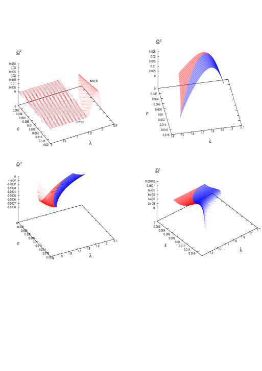
Figure 2: Variation of $\Omega^{2}$ with respect to $\mathcal{E}$ and $\lambda$, under the pseudo-Newtonian potential $\phi_{1}$. The plot in the top left corner gives the variation for the regions of a single critical point only. The remaining three figures are for the multi-transonic region. Clockwise from the top right corner will give the variations for the inner critical point, the outer critical point and the middle critical point, respectively.

Figure 3: Variation of $\Omega^{2}$ with respect to $\lambda$, for fixed values of $\mathcal{E}$, in a polytropic flow. Each plot shows the birth of two critical points at a given value of $\lambda$, which coalesce later at a higher value of $\lambda$.

Figure 4: Variation of $\Omega^{2}$ with respect to $\lambda$, for fixed values of $T$, in an isothermal flow. Unlike the case of polytropic flows, here the eigenvalues related to the inner critical point (a saddle point) continue to grow monotonically beyond the range of multi-transonicity.

For the Paczyński & Wiita (1980) potential, $\phi_{1}$, the variation of $\Omega^{2}$ against $\mathcal{E}$ and $\lambda$ is given in Fig. 2. The plot in the top left corner of this panel gives the dependence of $\Omega^{2}$ on $\mathcal{E}$ and $\lambda$ for the regions of the single critical point. The flat portion is related to the outer critical point, while the hump is related to the inner critical point. Both of these points are saddle points. The vacant wedge-shaped area between these two regions is the region of multi-transonicity, which has been separately represented for the behaviour of the three distinct critical points in the remaining three plots in the panel. The top right corner shows the variation of the inner critical point, which is a saddle point. The bottom left plot gives the variation of the eigenvalues for the centre-type middle critical point, while the properties of the outermost saddle-type critical point are given by the bottom right plot in Fig. 2.

A common feature of all the three separate plots for the eigenvalues of the multi-transonic region is that they contain information on both accretion and wind. Here the lightly shaded regions (coloured red in the online version) in the plots indicate accretion. The criterion to distinguish accretion from wind has been that the flow rate through the inner critical point (a saddle point), $\dot{\mathcal{M}}_{\mathrm{in}}$, has to be greater than the corresponding flow rate through the outer critical point (again a saddle point), $\dot{\mathcal{M}}_{\mathrm{out}}$. The exact reversal of this requirement will give the wind region, which has been given by the darkly shaded portion (coloured blue in the online version) of each plot. These points can be better appreciated from the colour images on the archive version of this paper.

Another property that one could discern from the surfaces in the $(\Omega^{2},{\mathcal{E}},\lambda)$ space is that the surface pertaining to the centre-type point has a minimum and then it rises, while the surface for the second saddle point has a miximum and then it dips. So the two of them taken together, they coalesce and “annihilate” each other at a large value of the angular momentum, and then all that is left behind is a single saddle point for the high angular momentum region of the parameter space.

This contention is very illustratively borne out by the top left plot of Fig. 3, in which $\Omega^{2}$ for all the three critical points has been plotted against $\lambda$, for a suitably chosen value of $\mathcal{E}$, in the case of a flow driven by the Paczyński & Wiita (1980) potential. Initially there is region of a single saddle point, followed by the birth of a centre-type point and another saddle point. Physically this is what it has to be, because with a centre-type point but without another saddle point, the flow solutions will all curl about the centre-type point, and there will be no means of connecting the event horizon with infinity through a solution. To avoid this, and to make accretion a feasible proposition, the existence of the inner saddle point should be most crucial. The other three plots in Fig. 3 demonstrate this same feature for the other pseudo-Newtonian potentials.

The whole situation is qualitatively similar for isothermal flows. The case for multi-transonicity in the parameter space of $T$ and $\lambda$ has been discussed in detail by Das et al. (2003). It is a simple extension from here to study the dependence of $\Omega^{2}$ on $T$ and $\lambda$. This has been shown in Fig. 4, which gives the variation of $\Omega^{2}$ against $\lambda$, for fixed values of $T$. Once again it is evident that the multi-transonic region begins and ends, respectively, with the production and annihilation of a pair of critical points — one a saddle and another a centre-type point. A crucial difference for isothermal flows, however, is that beyond the multi-transonic region, for high values of angular momentum, the eigenvalues in relation to the lone saddle point increase monotonically in magnitude.

A few points are worth emphasising upon once again at the end of this whole discussion, dwelling on both kinds of flows — polytropic and isothermal. Without encountering the difficulties of numerical integration, much predictive insight has been derived about the qualitative character of the flow, not the least of which, crucially, is the exclusive nature of the critical points, and in relation to that, important physical features of multi-transonicity itself.

5 Time-dependent stability analysis of stationary solutions

Under the condition of hydrostatic equilibrium in the vertical direction, the time-dependent generalisation of the governing equations for an axisymmetric pseudo-Schwarzschild disc is given as

$$\frac{\partial v}{\partial t}+v\frac{\partial v}{\partial r}+\frac{1}{\rho}\frac{\partial P}{\partial r}+\phi^{\prime}(r)-\frac{\lambda^{2}}{r^{3}}=0$$ (20)

and

$$\frac{\partial\Sigma}{\partial t}+\frac{1}{r}\frac{\partial}{\partial r}\left(\Sigma vr\right)=0$$ (21)

in which the surface density of the thin disc $\Sigma$, is to be expressed as $\Sigma\cong\rho H$ (Frank et al., 2002). Making use of Eq.(4) and the polytropic relation $P=K\rho^{\gamma}$, Eq.(21) can be rendered as

$$\frac{\partial}{\partial t}\left[\rho^{(\gamma+1)/2}\right]+\frac{\sqrt{\phi^{\prime}}}{r^{3/2}}\frac{\partial}{\partial r}\left[\rho^{(\gamma+1)/2}v\frac{r^{3/2}}{\sqrt{\phi^{\prime}}}\right]=0$$ (22)

Defining a new variable $f=\rho^{(\gamma+1)/2}vr^{3/2}/\sqrt{\phi^{\prime}}$, it is quite obvious from the form of Eq.(22) that the stationary value of $f$ will be a constant, $f_{0}$, which can be closely identified with the matter flux rate. This follows a similar approach to spherically symmetric flows made by Petterson et al. (1980) and Theuns & David (1992). For an axisymmetric disc, which has no dependence on any angle variable, this approach has also been adopted for a flow driven simply by a Newtonian potential (Ray, 2003). The present treatment, of course, is of a more general nature, the disc flow being driven by a general pseudo-Newtonian potential, $\phi(r)$. In this system, a perturbation prescription of the form $v(r,t)=v_{0}(r)+v^{\prime}(r,t)$ and $\rho(r,t)=\rho_{0}(r)+\rho^{\prime}(r,t)$, will give, on linearising in the primed quantities,

$$f^{\prime}=f_{0}\left[\left(\frac{\gamma+1}{2}\right)\frac{\rho^{\prime}}{\rho_{0}}+\frac{v^{\prime}}{v_{0}}\right]$$ (23)

with the subscript $0$ denoting stationary values in all cases. From Eq.(22), it then becomes possible to set down the density fluctuations $\rho^{\prime}$, in terms of $f^{\prime}$ as

$$\frac{\partial\rho^{\prime}}{\partial t}+\beta^{2}\frac{v_{0}\rho_{0}}{f_{0}}\left(\frac{\partial f^{\prime}}{\partial r}\right)=0$$ (24)

with $\beta^{2}=2(\gamma+1)^{-1}$, as before. Combining Eqs.(23) and (24) will then render the velocity fluctuations as

$$\frac{\partial v^{\prime}}{\partial t}=\frac{v_{0}}{f_{0}}\left(\frac{\partial f^{\prime}}{\partial t}+{v_{0}}\frac{\partial f^{\prime}}{\partial r}\right)$$ (25)

which, upon a further partial differentiation with respect to time, will give

$$\frac{{\partial}^{2}v^{\prime}}{\partial t^{2}}=\frac{\partial}{\partial t}\left[\frac{v_{0}}{f_{0}}\left(\frac{\partial f^{\prime}}{\partial t}\right)\right]+\frac{\partial}{\partial t}\left[\frac{v_{0}^{2}}{f_{0}}\left(\frac{\partial f^{\prime}}{\partial r}\right)\right]$$ (26)

From Eq.(20) the linearised fluctuating part could be extracted as

$$\frac{\partial v^{\prime}}{\partial t}+\frac{\partial}{\partial r}\left(v_{0}v^{\prime}+c_{\mathrm{s0}}^{2}\frac{\rho^{\prime}}{\rho_{0}}\right)=0$$ (27)

with $c_{\mathrm{s0}}$ being the speed of sound in the steady state. Differentiating Eq.(27) partially with respect to $t$, and making use of Eqs.(24), (25) and (26) to substitute for all the first and second-order derivatives of $v^{\prime}$ and $\rho^{\prime}$, will deliver the result

$$\frac{\partial}{\partial t}\left[\frac{v_{0}}{f_{0}}\left(\frac{\partial f^{\prime}}{\partial t}\right)\right]+\frac{\partial}{\partial t}\left[\frac{v_{0}^{2}}{f_{0}}\left(\frac{\partial f^{\prime}}{\partial r}\right)\right]+\frac{\partial}{\partial r}\left[\frac{v_{0}^{2}}{f_{0}}\left(\frac{\partial f^{\prime}}{\partial t}\right)\right]+\frac{\partial}{\partial r}\left[\frac{v_{0}}{f_{0}}\left(v_{0}^{2}-\beta^{2}c_{\mathrm{s0}}^{2}\right)\frac{\partial f^{\prime}}{\partial r}\right]=0$$ (28)

all of whose terms can be ultimately rendered into a compact formulation that looks like

$$\partial_{\mu}\left({\mathrm{f}}^{\mu\nu}\partial_{\nu}f^{\prime}\right)=0$$ (29)

in which the Greek indices are made to run from $0$ to $1$, with the identification that $0$ stands for $t$, and $1$ stands for $r$. An inspection of the terms in the left hand side of Eq.(28) will then allow for constructing the symmetric matrix

$${\mathrm{f}}^{\mu\nu}=\frac{v_{0}}{f_{0}}\pmatrix{1&v_{0}\cr v_{0}&v_{0}^{2}-\beta^{2}c_{\mathrm{s0}}^{2}}$$ (30)

Now the d’Alembertian for a scalar in curved space is given in terms of the metric ${\mathrm{g}}_{\mu\nu}$ by (Visser, 1998)

$$\Delta\psi\equiv\frac{1}{\sqrt{-\mathrm{g}}}\partial_{\mu}\left({\sqrt{-\mathrm{g}}}\,{\mathrm{g}}^{\mu\nu}\partial_{\nu}\psi\right)$$ (31)

with $\mathrm{g}^{\mu\nu}$ being the inverse of the matrix implied by ${\mathrm{g}}_{\mu\nu}$. Using the equivalence that ${\mathrm{f}}^{\mu\nu}=\sqrt{-\mathrm{g}}\,{\mathrm{g}}^{\mu\nu}$, and therefore $\mathrm{g}=\det\left({\mathrm{f}}^{\mu\nu}\right)$, it is immediately possible to set down an effective metric for the propagation of an acoustic disturbance as

$$\mathrm{g}^{\mu\nu}_{\mathrm{eff}}=\pmatrix{1&v_{0}\cr v_{0}&v_{0}^{2}-\beta^{2}c_{\mathrm{s0}}^{2}}$$ (32)

which can be shown to be entirely identical to the metric of a wave equation for a scalar field in curved space-time, obtained through a somewhat different approach (Visser, 1998). The inverse effective metric, $\mathrm{g}_{\mu\nu}^{\mathrm{eff}}$, can be easily derived by inversion of the matrix given in Eq.(32), and this will give $v_{0}^{2}=\beta^{2}c_{\mathrm{s0}}^{2}$ as the horizon condition of an acoustic black hole for inflow solutions (Visser, 1998).

A little readjustment of terms in Eq.(28) will finally give an equation for the perturbation as

$$\frac{{\partial}^{2}f^{\prime}}{\partial t^{2}}+2\frac{\partial}{\partial r}\left(v_{0}\frac{\partial f^{\prime}}{\partial t}\right)+\frac{1}{v_{0}}\frac{\partial}{\partial r}\left[v_{0}\left(v_{0}^{2}-\beta^{2}c_{\mathrm{s0}}^{2}\right)\frac{\partial f^{\prime}}{\partial r}\right]=0$$ (33)

whose form, as can be easily seen, remains invariant under any possible choice of a pseudo-potential. This is entirely to be expected since the potential, being independent of time, will have its explicit presence in only the stationary background flow. Once again it is a simple exercise to check that an expression with the same form as Eq.(33) could be derived for the case of isothermal flows, but which will, however, have $\beta=1$ and $c_{\mathrm{s0}}$ as a constant.

The perturbation is now fashioned to behave like a travelling wave, whose wavelength is constrained to remain small, i.e. it is to be smaller than any characteristic length scale in the system. This kind of a treatment has been carried out before on spherically symmetric flows (Petterson et al., 1980) and on axisymmetric flows driven by a Newtonian potential (Ray, 2003). In both these cases the radius of the accretor was chosen as the characteristic length scale in question, and the wavelength of the perturbation was chosen to be much smaller than this length scale. In the present study, which is devoted to an axisymmetric flow driven on to a black hole by a pseudo-Newtonian potential, the radius of the event horizon could be a choice for such a length scale. As a result, the frequency, $\omega$, of the waves should be large. A solution of the kind $f^{\prime}(r,t)=g_{\omega}(r)\exp(-{\mathrm{i}}\omega t)$ is used in Eq.(33), to give the expression

$$\left(v_{0}^{2}-\beta^{2}c_{\mathrm{s0}}^{2}\right)\frac{{\mathrm{d}^{2}}g_{\omega}}{{\mathrm{d}}r^{2}}+\left[3v_{0}\frac{{\mathrm{d}}v_{0}}{{\mathrm{d}}r}-\frac{1}{v_{0}}{\frac{\mathrm{d}}{{\mathrm{d}}r}}\left(v_{0}\beta^{2}c_{\mathrm{s0}}^{2}\right)-2{\mathrm{i}}\omega v_{0}\right]\frac{{\mathrm{d}}g_{\omega}}{{\mathrm{d}}r}-\left(2{\mathrm{i}}\omega\frac{{\mathrm{d}}v_{0}}{{\mathrm{d}}r}+\omega^{2}\right)g_{\omega}=0$$ (34)

beyond which stage, mindful of the constraint that $\omega$ is large, the spatial part of the perturbation, $g_{\omega}(r)$, is first prescribed to be a power series in the form

$$g_{\omega}(r)=\exp\left[\sum_{n=-1}^{\infty}\frac{k_{n}(r)}{\omega^{n}}\right]$$ (35)

and this is then used in Eq.(34). Following this, the three successive highest order terms in $\omega$ will be obtained as $\omega^{2}$, $\omega$ and $\omega^{0}$. Collecting all the coefficients of each of these terms, summing these coefficients up, and then separately setting each individual sum to zero, will yield, respectively, for $\omega^{2}$, $\omega$ and $\omega^{0}$, the conditions

$$\left(v_{0}^{2}-\beta^{2}c_{\mathrm{s0}}^{2}\right)\left(\frac{{\mathrm{d}}k_{-1}}{{\mathrm{d}}r}\right)^{2}-2{\mathrm{i}}v_{0}\frac{{\mathrm{d}}k_{-1}}{{\mathrm{d}}r}-1=0$$ (36)

$$\left(v_{0}^{2}-\beta^{2}c_{\mathrm{s0}}^{2}\right)\left(\frac{{\mathrm{d}}^{2}k_{-1}}{{\mathrm{d}}r^{2}}+2\frac{{\mathrm{d}}k_{-1}}{{\mathrm{d}}r}\frac{{\mathrm{d}}k_{0}}{{\mathrm{d}}r}\right)+\left[3v_{0}\frac{{\mathrm{d}}v_{0}}{{\mathrm{d}}r}-\frac{1}{v_{0}}\frac{\mathrm{d}}{{\mathrm{d}}r}\left(v_{0}\beta^{2}c_{\mathrm{s0}}^{2}\right)\right]\frac{{\mathrm{d}}k_{-1}}{{\mathrm{d}}r}-2{\mathrm{i}}v_{0}\frac{{\mathrm{d}}k_{0}}{{\mathrm{d}}r}-2{\mathrm{i}}\frac{{\mathrm{d}}v_{0}}{{\mathrm{d}}r}=0$$ (37)

and

$$\left(v_{0}^{2}-\beta^{2}c_{\mathrm{s0}}^{2}\right)\left[\frac{{\mathrm{d}}^{2}k_{0}}{{\mathrm{d}}r^{2}}+2\frac{{\mathrm{d}}k_{-1}}{{\mathrm{d}}r}\frac{{\mathrm{d}}k_{1}}{{\mathrm{d}}r}+\left(\frac{{\mathrm{d}}k_{0}}{{\mathrm{d}}r}\right)^{2}\right]+\left[3v_{0}\frac{{\mathrm{d}}v_{0}}{{\mathrm{d}}r}-\frac{1}{v_{0}}\frac{\mathrm{d}}{{\mathrm{d}}r}\left(v_{0}\beta^{2}c_{\mathrm{s0}}^{2}\right)\right]\frac{{\mathrm{d}}k_{0}}{{\mathrm{d}}r}-2{\mathrm{i}}{v_{0}}\frac{{\mathrm{d}}k_{1}}{{\mathrm{d}}r}=0$$ (38)

Out of these, the first two, i.e. Eqs.(36) and (37), will deliver the solutions

$$k_{-1}=\int\frac{{\mathrm{i}}}{v_{0}\pm\beta c_{\mathrm{s0}}}\,{\mathrm{d}}r$$ (39)

and

$$k_{0}=-\frac{1}{2}\ln\left(\beta v_{0}c_{\mathrm{s0}}\right)+{\mathrm{constant}}$$ (40)

respectively. The two expressions above give the leading terms in the power series of $g_{\omega}(r)$. For self-consistency it will be necessary to show that successive terms follow the condition $\omega^{-n}|k_{n}(r)|\gg\omega^{-(n+1)}|k_{n+1}(r)|$, i.e. the power series given by $g_{\omega}(r)$ converges rapidly as $n$ increases. This requirement can be shown to be very much true, if the behaviour of the first three terms in $k_{n}(r)$ is any indication. From Eqs. (39), (40) and (38), respectively, these terms can be shown to go asymptotically as $k_{-1}\sim r$, $k_{0}\sim\ln r$ and $k_{1}\sim r^{-1}$, given the condition that $v_{0}\sim r^{-5/2}$ on large length scales, while $c_{\mathrm{s0}}$ approaches its constant ambient value. Under the regime of high-frequency travelling waves, this will imply $\omega|k_{-1}|\gg|k_{0}|\gg\omega^{-1}|k_{1}|$, and, therefore, it should suffice here entirely to consider the two leading terms only, as given by Eqs.(39) and (40), in the power series expansion of $g_{\omega}(r)$, as Eq. (35) gives it. So with the help of these two terms, one may then set down an expression for the perturbation as

$$f^{\prime}(r,t)\simeq\frac{A_{\pm}}{\sqrt{\beta v_{0}c_{\mathrm{s0}}}}e^{-{\mathrm{i}}\omega t}\exp\left(\int\frac{{\mathrm{i}}\omega}{v_{0}\pm\beta c_{\mathrm{s0}}}\,{\mathrm{d}}r\right)$$ (41)

which should be seen as a linear superposition of two waves with arbitrary constants $A_{+}$ and $A_{-}$. Both these two waves move with velocity $\beta c_{\mathrm{s0}}$ relative to the fluid, one against the bulk flow and the other along with it, while the bulk flow itself has velocity $v_{0}$. With the help of Eq.(24) it should then be easy to express the density fluctuations in terms of $f^{\prime}$ as

$$\rho^{\prime}\simeq\beta^{2}\frac{v_{0}\rho_{0}}{f_{0}}\left(\frac{f^{\prime}}{v_{0}\pm\beta c_{\mathrm{s0}}}\right)$$ (42)

and as a further step, with the help of Eq.(23), it should also be possible to set down the velocity fluctuations as

$$v^{\prime}\simeq\pm\beta\frac{v_{0}c_{\mathrm{s0}}}{f_{0}}\left(\frac{f^{\prime}}{v_{0}\pm\beta c_{\mathrm{s0}}}\right)$$ (43)

with the positive and the negative signs indicating incoming and outgoing waves, respectively.

In a unit volume of the fluid, the kinetic energy content is

$${\mathcal{E}}_{\mathrm{kin}}=\frac{1}{2}\left(\rho_{0}+\rho^{\prime}\right)\left(v_{0}+v^{\prime}\right)^{2}$$ (44)

while the potential energy per unit volume of the fluid is the sum of the gravitational energy, the rotational energy and the internal energy, and is given by

$${\mathcal{E}}_{\mathrm{pot}}=\left(\rho_{0}+\rho^{\prime}\right)\phi-\left(\rho_{0}+\rho^{\prime}\right)\frac{\lambda^{2}}{2r^{2}}+\rho_{0}\epsilon+\rho^{\prime}\frac{\partial}{\partial\rho_{0}}\left(\rho_{0}\epsilon\right)+\frac{1}{2}{\rho^{\prime}}^{2}\frac{{\partial}^{2}}{\partial\rho_{0}^{2}}\left(\rho_{0}\epsilon\right)$$ (45)

where $\epsilon$ is the internal energy per unit mass (Landau & Lifshitz, 1987). In Eqs.(44) and (45), the first-order terms vanish on time-averaging. In that case the leading contribution to the total energy in the perturbation comes from the second-order terms, which are given by

$${\mathcal{E}}_{\mathrm{pert}}=\frac{1}{2}\rho_{0}{v^{\prime}}^{2}+v_{0}\rho^{\prime}v^{\prime}+\frac{1}{2}{\rho^{\prime}}^{2}\frac{{\partial}^{2}}{\partial\rho_{0}^{2}}\left(\rho_{0}\epsilon\right)$$ (46)

If the perturbation is constrained to be adiabatic, then the condition ${\mathrm{d}}s=0$ can be imposed on the thermodynamic relation, ${\mathrm{d}}\epsilon=T{\mathrm{d}}s+\left(P/\rho^{2}\right){\mathrm{d}}\rho$, which will then give

$$\frac{{\partial}^{2}}{\partial\rho_{0}^{2}}\left(\rho_{0}\epsilon\right){\bigg{|}}_{s}=\frac{c_{\mathrm{s0}}^{2}}{\rho_{0}}$$ (47)

Combining the results from Eqs.(41), (42), (43), (46) and (47), and upon time-averaging over the square of the fluctuations, will give

$${\mathcal{E}}_{\mathrm{pert}}\simeq\frac{1}{2}\frac{\beta^{2}A_{\pm}^{2}}{f_{0}^{2}}\frac{v_{0}\rho_{0}}{\left(v_{0}\pm\beta c_{{\mathrm{s}0}}\right)^{2}}\left[\frac{\beta c_{\mathrm{s0}}}{2}\left(1+\frac{1}{\beta^{2}}\right)\pm v_{0}\right]$$ (48)

with the factor $1/2$ in Eq.(48) arising from the time-averaging of the fluctuations.

The total energy flux in the perturbation is obtained by multiplying ${\mathcal{E}}_{\mathrm{pert}}$ by the propagation velocity $(v_{0}\pm\beta c_{\mathrm{s0}})$ and then by integrating over the area of the cylindrical face of the accretion disc, which is $2\pi rH$. Here $H$ is to be substituted from Eq.(4), and together with the condition that $H\ll r$ in the thin-disc approximation, and the fact that the speed of sound has a functional dependence on the density going as $c_{\mathrm{s0}}^{2}=\gamma K\rho_{0}^{\gamma-1}$, an expression for the energy flux will be obtained as

$${\mathcal{F}}=\frac{\pi A_{\pm}^{2}\sqrt{K}\beta^{2}}{f_{0}}\left[\pm 1+\frac{1-\beta^{2}}{2\beta\left(M\pm\beta\right)}\right]$$ (49)

where $M\equiv M(r)=v_{0}/c_{\mathrm{s0}}$, is the Mach number, which under a generic outer boundary condition, tends to vanishingly small values on large length scales of the accretion disc. All other factors in the expression of $\mathcal{F}$ are constants. It is quite evident once again that the forms of both ${\mathcal{E}}_{\mathrm{pert}}$ and ${\mathcal{F}}$ are invariant under the choice of any pseudo-potential, and therefore all arguments for the stability of the flow will be valid for any choice. Indeed, this should be especially true on large length scales of the flow, where all $\phi(r)$ will asymptotically tend to the Newtonian limit.

As regards the question of the behaviour of the perturbation, it can be seen that for sub-critical solutions, the condition $M(r)<\beta$ always holds everywhere for both the incoming and the outgoing modes of the perturbation, which, of course, implies that the total energy in the wave remains finite as the wave propagates. The perturbation manifests no unbridled divergence anywhere, and all sub-critical solutions are, therefore, stable.

For the critical solution, it is evident that with the choice of the upper sign in Eq.(49), i.e. for incoming waves, which propagate along with the bulk flow, once again there is no growth behaviour for the perturbation to be seen anywhere and all stationary inflow solutions are, therefore, stable for this propagating mode of the perturbation.

For the choice of the lower sign, i.e. for outwardly propagating radial waves, it is first of all very obvious from Eq.(49), that there is no unrestrained growth of the energy flux of the perturbation in the region where $M(r)<\beta$, and so the disc system remains stable in this sub-critical region. The case for stability is even better argued in the region of the flow where $M(r)>\beta$. In this region, which has a finite spatial extent, all outwardly propagating waves will be swept away in finite time by the inward bulk flow right up to the event horizon of the black hole, and this physical effect will also ensure the stability of the flow in this region. This very same line of reasoning was adopted by Garlick (1979) to argue for the stability of the critical solution in the supersonic region of a spherically symmetric flow. As an interesting aside, it may also be mentioned here that this argument is well in consonance with the analogy of an acoustic black hole. Any disturbance within the sonic horizon for inflows, will not be able to propagate outwards through the horizon. Therefore, it can be established generally that in an inviscid pseudo-Schwarzschild system, all physically well-behaved inflow solutions will be stable under the influence of a linearised high-frequency radial perturbation, propagating either inwardly or outwardly.

6 Concluding remarks

Saddle points are inherently unstable, and to make a solution pass through such a point, after starting from an outer boundary condition, will entail an infinitely precise fine-tuning of that boundary condition (Ray & Bhattacharjee, 2002). Nevertheless, transonicity, i.e. generating a solution through a saddle point, is not a matter of doubt. The key to this paradox lies in considering a time-dependent evolution of the flow. In this paper, time-dependence in the flow has indeed been taken up, although in a perturbative manner, which has shown that all solutions of physical interest are stable. So the selection of a solution through a saddle point will have to fall back on non-perturbative arguments (Ray & Bhattacharjee, 2002). This is a relatively simple proposition for the case of a flow in the Newtonian framework. The difficulties against this line of attack, however, are understandably much greater when the flow properties are studied in a general relativistic framework. Notwithstanding this fact, as a preliminary foray into this question, it should be important to have some understanding of the behaviour of the general relativistic flow solutions in their stationary phase portrait. This will be a matter of a subsequent investigation, for flows both on to a Schwarzschild black hole and a Kerr black hole.

References

- Abraham et al. (2006) Abraham, H., Bilić, N., Das, T. K., 1998, Classical and Quantum Gravity, 23, 2371
- Abramowicz & Zurek (1981) Abramowicz, M. A., Zurek, W. H. 1981, ApJ, 246, 314
- Afshordi & Paczyński (2003) Afshordi, N., Paczyński, B., 2003, ApJ, 592, 354
- Artemova et al. (1996) Artemova, I. V., Björnsson, G., Novikov, I. D., 1996, ApJ, 461, 565
- Barai et al. (2004) Barai, P., Das, T. K., Wiita, P. J., 1996, ApJ, 613, L49
- Bohr et al. (1993) Bohr, T., Dimon, P., Putkaradze, V., 1993, J. Fluid Mech., 254, 635
- Chakrabarti (1989) Chakrabarti, S. K., 1989, ApJ, 347, 365
- Chakrabarti (1990) Chakrabarti, S. K., 1990, Theory of Transonic Astrophysical Flows, World Scientific, Singapore
- Chandrasekhar (1939) Chandrasekhar, S., 1939, An Introduction to the Study of Stellar Structure, The University of Chicago Press, Chicago
- Das (2002) Das, T. K., 2002, ApJ, 577, 880
- Das (2004) Das, T. K., 2004, MNRAS, 375, 384
- Das et al. (2006) Das, T. K., Bilić, N., Dasgupta, S., 2006, arXiv:astro-ph/0604477
- Das et al. (2003) Das, T. K., Pendharkar, J. K., Mitra, S., 2003, ApJ, 592, 1078
- Das & Sarkar (2001) Das, T. K., Sarkar, A., 2001, A&A, 374, 1150
- Frank et al. (2002) Frank, J., King, A., Raine, D., 1992, Accretion Power in Astrophysics, Cambridge University Press, Cambridge
- Fukue (1987) Fukue, J., 1987, PASJ, 39, 309
- Garlick (1979) Garlick, A. R., 1979, A&A, 73, 171
- Jordan & Smith (1999) Jordan, D. W., Smith, P., 1999, Nonlinear Ordinary Differential Equations, Oxford University Press, Oxford
- Kafatos & Yang (1994) Kafatos, M., Yang, R. X., 1994, A&A, 268, 925
- Landau & Lifshitz (1987) Landau, L. D., Lifshitz, E. M., 1987, Fluid Mechanics, Butterworth-Heinemann, Oxford
- Lasota & Abramowicz (1997) Lasota, J. P., Abramowicz, M. A., 1998, Classical and Quantum Gravity, 15, 1767
- Lu et al. (1997) Lu, J. F., Yu, K. N., Yuan, F., Young, E. C. M., 1997, A&A, 321, 665
- Matsumoto et al. (1984) Matsumoto, R., Kato, S., Fukue, J., Okazaki, A. T., 1984, PASJ, 36, 71
- Nowak & Wagoner (1991) Nowak, A. M., Wagoner, R. V., 1991, ApJ, 378, 656
- Paczyński & Wiita (1980) Paczyński, B., Wiita P. J., 1980, A&A, 88, 23
- Pariev (1996) Pariev, V. I., 1996, MNRAS, 283, 1264
- Peitz & Appl (1997) Peitz, J., Appl, S., 1997, MNRAS, 286, 681
- Petterson et al. (1980) Petterson, J. A., Silk, J., Ostriker, J. P., 1980, MNRAS, 191, 571
- Ray (2003) Ray, A. K., 2003, MNRAS, 344, 83
- Ray & Bhattacharjee (2002) Ray, A. K., Bhattacharjee, J.K., 2002, Phys. Rev. E, 66, 066303
- Theuns & David (1992) Theuns, T., David, M., 1991, ApJ, 384, 587
- Visser (1998) Visser, M., 1998, Classical and Quantum Gravity, 15, 1767
- Yang & Kafatos (1995) Yang, R. X., Kafatos, M., 1995, A&A, 295, 238