Photometric Redshifts in the IRAC Shallow Survey

Abstract

Accurate photometric redshifts are calculated for nearly 200,000 galaxies to a 4.5 micron flux limit of $\sim 13$ $\mu$Jy in the 8.5 deg² Spitzer/IRAC Shallow survey. Using a hybrid photometric redshift algorithm incorporating both neural–net and template–fitting techniques, calibrated with over 15,000 spectroscopic redshifts, a redshift accuracy of $\sigma=0.06\,(1+z)$ is achieved for 95% of galaxies at $0<z<1.5$. The accuracy is $\sigma=0.12\,(1+z)$ for 95% of AGN at $0<z<3$. Redshift probability functions, central to several ongoing studies of the galaxy population, are computed for the full sample. We demonstrate that these functions accurately represent the true redshift probability density, allowing the calculation of valid confidence intervals for all objects. These probability functions have already been used to successfully identify a population of Spitzer–selected high redshift ($z>1$) galaxy clusters. We present one such spectroscopically confirmed cluster at $\left<z\right>=1.24$, ISCS J1434.5+3427. Finally, we present a measurement of the 4.5$\mu$m–selected galaxy redshift distribution.

1. Introduction

In modern wide-field imaging surveys, accurate photometric redshifts have become an indispensable tool for studying the evolving galaxy population. This approach allows studies of the galaxy luminosity and correlation functions, power spectrum analyses, and rare–object searches, reserving costly 8–m class spectroscopic follow–up for analyses where such data are crucial.

Much of the new extragalactic science enabled by the Spitzer Space Telescope will not just be more efficient with photometric redshifts, but rather completely reliant on them. Spitzer is uniquely capable of detecting huge numbers of galaxies from their rest 1.6 $\mu$m stellar emission or mid–IR PAH features all the way to $z=2$ and beyond. These objects are often quite faint in the optical, due to either quiescence or heavy extinction, making spectroscopic follow–up difficult or impossible with existing facilities.

The IRAC Shallow survey (Eisenhardt et al., 2004) is a wide–field 8.5 deg² Spitzer/IRAC imaging survey in the NOAO Deep Wide–Field Survey (NDWFS; Jannuzi and Dey, 1999) Boötes field, designed to study galaxy formation and evolution across a wide range of redshifts, mass scales, colors and environments. Extensive complementary data includes a 5 ksec per pointing X-ray mosaic (XBoötes; Murray et al. 2005; Kenter et al. 2005; Brand et al. 2006), and Spitzer/MIPS 24/70/160 $\mu$m imaging (GTO program, Soifer PI) over the full survey area. In addition, the FLAMINGOS Extragalactic Survey (FLAMEX; Elston et al., 2006) provides deep $J$ and $K_{s}$ imaging over the central $\approx 4.7$ deg². Finally, there are 17,017 spectroscopic redshifts of galaxies to $z\sim 0.8$ and AGN to $z=5.85$ from the AGN and Galaxy Evolution Survey (AGES; Cool et al. 2006; Kochanek et al. in preparation), along with $\sim 500$ redshifts of fainter, higher redshift galaxies from various other surveys in Boötes, which are available for calibration of the photometric redshift algorithm.

In this paper, we combine the optical photometry from the NDWFS, the near–IR photometry from FLAMEX, and the mid–IR photometry from the IRAC Shallow survey to compute accurate photometric redshifts for 4.5$\mu$m–selected galaxies to $z=1.5$ and AGN to $z=3$. A hybrid method, combining a standard template–fitting algorithm with an artificial neural net–based approach, is developed to make optimal use of the large AGES spectroscopic calibration sample.

Redshift probability functions are derived for the full sample, nearly 200,000 objects over 8.5 deg², and are employed to calculate the 4.5$\mu$m redshift distribution. They are also the input to a high–redshift cluster search underway in Boötes, which has already yielded the highest redshift galaxy cluster to date ($\left<z\right>=1.41$; Stanford et al., 2005). This paper presents a new, spectroscopically confirmed high redshift cluster at $\left<z\right>=1.24$.

This paper is organized as follows. In §2 the various data sets used in this paper are briefly described. In §3 the photometric redshift algorithm is presented, and the results are compared to the AGES spectroscopy. The calculation of redshift probability functions is described in §4, and in §5 we employ them to compute the 4.5$\mu$m redshift distribution and present a new $\left<z\right>=1.24$ galaxy cluster discovered using them. We summarize our results in §6. All magnitudes are Vega–based.

2. Photometric and Spectroscopic Data

2.1. Optical and NIR Photometry

Optical $B_{W}$, $R$, and $I$ imaging data were taken from the third data release (DR3) of the public NDWFS survey in the Boötes field. These data, obtained with the Mosaic–I camera on the NOAO 4–m, are described fully in Jannuzi et al. (in preparation) and available through the NOAO Science Archive (http://archive.noao.edu/nsa/).

Robust photometric errors were estimated via Monte–Carlo simulation, and extensive flagging of both pixel and image artifacts allows selection of high-quality photometric samples over the full survey area. The optical photometry reaches 3$\sigma$ 5″ diameter Vega depths of $B_{W}=25.3$, $R=24.1$, and $I=23.6$. The large apertures are taken to better match the IRAC PSF and to minimize the effect of seeing variations in the optical data, as discussed below. The NDWFS is significantly deeper for point source or small aperture photometry.

The FLAMEX survey (Elston et al., 2006) is a near–IR $J$– and $K_{s}$–band imaging survey undertaken with the FLAMINGOS camera on the NOAO 2.1–m. Photometric errors were determined via extensive Monte Carlo simulations, accounting for PSF variations across the field. The survey covers the central $\sim$4.7 deg² subset of the Boötes field to a 5″ diameter aperture, 50% completeness limit of $K_{s}=19.4$.

2.2. IRAC imaging

The IRAC Shallow survey, introduced in Eisenhardt et al. (2004), is a Spitzer/IRAC imaging survey in the NDWFS Boötes field, covering 8.5 deg² with 3 or more 30 second exposures per position at 3.6, 4.5, 5.8, and 8.0 $\mu$m to 5$\sigma$ flux limits in a 5″ aperture of 10.0, 13.3, 78.0, and 68.3 $\mu$Jy, or Vega magnitude limits of 18.6, 17.8, 15.4, and 14.9, respectively.

Separate photometric catalogues were extracted in each channel using SExtractor $2.3.2$ (Bertin and Arnouts, 1996) in double–image mode, producing matched catalogs in the other 3 IRAC bands. The detection images in each channel were weighted by the error images generated by the MOPEX mosaicking software (Makovoz and Khan, 2005). This paper focusses on the 4.5 $\mu$m–selected catalog, which is the natural selection band for the $1<z<2$ cluster search described below (e.g., Eisenhardt et al., in preparation).

Quality control was maintained through the extensive use of flags. In particular, to ensure reliable colors, objects with less than 3 exposures in any single pixel within the aperture of interest were rejected from the final catalogs. This primarily removes objects from the edges of the field, with only $\sim$1% of the 4.5 $\mu$m sample rejected in the main overlap region. This spatial selection function is well quantified and will not affect any science analyses. This flagging was carried out for all of our apertures, which span diameters of 1–20″, chosen to match the DR3 NDWFS catalogs that form our primary complementary data set. All IRAC aperture photometry was corrected to large (24.4″ diameter) apertures to account for PSF losses. For the 5$\sigma$ 5″ diameter aperture of interest in this work, there are 211, 260 objects which have the full exposure time in both the [3.6] and [4.5] bands.

2.2.1 Catalog Matching

There is a small offset, of 0.38″ in right ascension and 0.15″ in declination, between the astrometric solutions of the near– and mid–IR catalogs, which are tied to the 2MASS reference frame, and the optical catalog, which is tied to the USNO–A2 (Monet et al., 2003). This offset, caused in part by errors in centroiding the bright Tycho–II stars used to zeropoint the USNO–A2 astrometry, was removed prior to matching (for further details, see Jannuzi et al., in preparation).

Detections in the optical and near–IR were matched to the 4.5 $\mu$m sources if the centroids were within $1\arcsec$ of each other. For extended objects, detections in the different bands were matched if the centroids were within an ellipse defined using the second order moments of the light distribution of the object. IRAC–selected objects with no match in a given optical or near–IR band were assigned a Monte Carlo estimated 1$\sigma$ flux limit representing the sky variation in a 5″ diameter aperture.

2.2.2 Photometric Redshift Sample

We define the photometric redshift sample as the subset of the [4.5]–selected matched catalog for which both the [3.6] and [4.5] data have the full 90s exposure time, and for which at least 2 of the 3 optical bands contain useful (i.e., unmasked) photometric data. Note that object detections in the optical, near–IR, and [3.6] bands are not required; 1$\sigma$ limits are used for non–detections. This results in a final multi–wavelength photometric redshift sample of 194,466 objects.

2.3. Spectroscopic Redshifts

The large sample of spectroscopic redshifts from AGES (Kochanek et al. in preparation) provides a crucial training sample for the photometric redshift algorithm. AGES is a wide–field MMT/Hectospec (Fabricant et al., 2005) redshift survey, version 2.0 of which contains high quality spectroscopic redshifts for 17,017 objects, including galaxies to $z\sim 0.8$ and AGN to $z=5.85$ (Cool et al., 2006). From this sample, 15,052 objects correspond to sources in the photometric redshift sample defined above.

The AGES survey was designed to allow magnitude–limited samples to be selected as a function of wavelength from the X–ray to the radio. In the IRAC 4.5$\mu$m band, the AGES survey is $\approx 100$% complete to 15.2 mag (150 $\mu$Jy), and statistically complete (with 30% random sampling) to 15.7 mag (95 $\mu$Jy).

However, more than half the spectroscopic sample lies beyond the fainter of these limits, driven primarily by the optical magnitude limits of $I=20$ for extended objects and $I=21.5$ for point sources, where the latter limit was designed to include relatively large numbers of AGN and quasars. In addition, the complete samples in the X-ray, UV, Far–IR and radio result in the survey being overweight in both active galaxies and those which are strongly starforming.

We have also assembled a deep ($R\sim 25$) heterogeneous sample of spectroscopic redshifts from several ongoing projects in the Boötes field for the purposes of calibrating the photometric redshifts. These projects include spectroscopic studies of optical, near-IR, IRAC and MIPS–selected sources, including our own spectroscopy of $1.1<z<1.4$ galaxy cluster members described below. As many of the principal investigators of these projects are also co–investigators of the present work (AD, BTJ, BTS, DS, SAS), we will call this the “in–house” sample for brevity.

3. Method: Photometric Redshifts

The impressive accuracy of photometric redshift algorithms of various types (Fernandez-Soto et al., 2002; Benítez, 2000; Fontana et al., 2000; Sawicki et al., 1997; Connolly et al., 1997; Firth et al., 2002; Brodwin et al., 2006; Hsieh et al., 2005; Wolf et al., 2003) is a good indication that the field is rapidly maturing at least as concerns optical/NIR surveys. It is less clear which methodology is best for redshift estimation from photometry extending into the $L$ and $M$ bands and beyond. A host of physics not included in current population synthesis models, including ubiquitous PAH emission and molecular and silicate absorption, could potentially complicate photometric redshift estimation in the first generation of Spitzer surveys.

Well–calibrated empirical methods such as fitting functions (e.g. Connolly et al., 1995; Brunner et al., 2000) and neural nets (Firth et al., 2003; Collister and Lahav, 2004; Vanzella et al., 2004) are capable of matching or surpassing the accuracy of template–fitting methods. They can be particularly powerful for analyses in which it is sufficient to predict accurate redshifts for a relatively small subset of the general galaxy population, albeit one with a large, representative spectroscopic training set. For instance, Blake et al. (2006) and Padmanabhan et al. (2006) measured the galaxy power spectrum using only bright, low-redshift, early type galaxies, selected with a variety of color and magnitude cuts. The large 4000 Å breaks and lack of SED ambiguity produces highly accurate redshifts in these samples.

In this paper we wish to develop a methodology with optimal photometric redshift accuracy over a much larger redshift baseline and spanning all galaxy types. Not surprisingly there is no spectroscopic sample spanning the full range of galaxy color, magnitude, spectral type, and redshift in the present survey. Despite the large size of the AGES spectroscopic sample, it consists of the low redshift, high luminosity component of the general IRAC photometric redshift sample. The situation for QSOs and AGN is more encouraging. The broad range of targeting methods and deeper limiting magnitudes likely lead to a broadly representative sample of unobscured AGN for all redshifts.

On the other hand, template–fitting methods calibrated with even modest spectroscopic redshift samples produce photometric redshifts which are generally robust outside of the narrow parameter space in which they are specifically validated. For this reason template–fitting algorithms are the de facto standard in the literature. An important advantage of this technique is the straightforward generation of redshift probability functions from the likelihood analysis, which are key to many science applications. This method is only accurate if the galaxy templates are representative of the observed galaxies. Strong PAH-emitting galaxies, for which reliable templates do not yet exist, along with quasars and AGN which have minimal continuum breaks, present a challenge for this technique.

In the IRAC Shallow survey we therefore employ a hybrid approach in which a template–fitting algorithm is used as the core method, supplemented by a well-calibrated neural net technique for the small subset of objects which both require and merit it.

3.1. Empirical Template–Fitting Algorithm

The template–fitting algorithm closely follows that described in detail in Brodwin et al. (2006). Coleman, Wu & Weedman (1980, CWW) galaxy SEDs, supplemented by the Kinney et al. (1996) empirical starburst (SB3 and SB2) SEDs are used as basis templates. These templates were extended to the far–UV and mid–IR using Bruzual and Charlot (2003) models. To improve the redshift accuracy linear interpolates were derived, resulting in 19 templates finely spanning the template space between the CWW Elliptical and SB2.

Population synthesis codes do not yet accurately model the complicated physical processes, in particular strong PAH emission, which can dominate the rest–frame $\lambda\gtrsim 5$ $\mu$m emission from normal galaxies. In view of this, and given that only the brightest $\sim 10\%$ of our sample has well–measured fluxes in the $5.8$ and $8.0$ $\mu$m bands, we elected to limit the fitting to the $\lambda<5$ $\mu$m regime where the models are expected to better approximate the true SEDs. This mild restriction still permits us to sample the stellar peak at 1.6 $\mu$m, a useful redshift indicator (e.g., Simpson and Eisenhardt 1999; Sawicki 2002) out to $z\sim 2$. The PAH emission at $\lambda\sim 3.3$ $\mu$m, which could potentially cause a template mismatch for strongly starforming galaxies, is quite modest in terms of equivalent width (EW $=0.02$$\mu$m; Lu et al., 2003). Indeed, this feature has only 0.5% of the power of the PAH features longward of 5$\mu$m (Helou et al., 2000). Since it redshifts out of the $[4.5]$ band by $z\sim 0.5$, any deleterious effect on redshift estimation should be limited to low redshifts.

Redshifts were fitted between $0\leq z\leq 5$ using 5″ diameter aperture $B_{W}RI+JK_{s}+[3.6][4.5]$ photometry where available. Reliable detections are not required as this would impose a strong selection effect; limits are used for areas of sky which were observed but for which no object was detected. Many deeper IRAC surveys suffer from considerable confusion in the bluer bands, leading to substantial difficulties in deriving accurate photometry. Due to the combination of area and depth targeted in the Shallow survey, the images are not confused, allowing straightforward aperture photometry.

To obtain robust galaxy colors, it is common in ground-based imaging surveys to smooth the images in all bands to a common worst seeing. Due to the relatively large PSF mismatch between Spitzer ($\sim$2″) and the ground–based optical data (0.8″-1.3″), it is not clear that this is the best approach. The large apertures required to enclose a substantial fraction of infrared light, empirically 5″, are sufficient to minimize the effects of seeing variations in the optical and near–IR images. We have verified that photometric redshifts computed with smaller apertures (3″) exhibit redshift– and position–dependent systematic errors, likely due to ground–based seeing variations. These effects vanish with the larger 5″ aperture photometry.

3.2. Correcting Templates and Zero Points

Comparison of preliminary photometric redshifts with AGES spectroscopy indicated an error in the mid–IR color of model elliptical galaxies. The spectral synthesis codes at $\lambda>1$ $\mu$m model a zero–color Rayleigh–Jeans tail typical of simple stellar populations. Recent Spitzer studies of nearby galaxies (Pahre et al., 2004) indicate that, while reasonable for late type galaxies, early–type galaxies are in fact blue in the mid–IR, with $[3.6]-[4.5]\approx-0.15$, due to CO absorption. To account for this the elliptical template (in $F_{\lambda}$) was scaled down between $1<\lambda(\mu\mbox{m})<5$ by a factor of $m\,(\lambda(\mu\mbox{m})-1)$, where the slope, $m=-0.11$, was determined by maximizing the photometric redshift accuracy for high S/N AGES elliptical galaxies. This change was carried through the template interpolations.

The large AGES spectroscopic sample was also used extensively to analyze the absolute inter–survey photometric calibration. For those objects well characterized by the model templates, the secure spectroscopic redshifts allow the AGES sample to be effectively used as spectrophotometric standards to determine inter–survey photometric offsets. These were found to be negligible in the optical and small in the near–IR, $\Delta J=-0.10$ mag and $\Delta K_{s}=-0.02$ mag. However, in the mid-IR the offsets between the observed photometry and the Bruzual and Charlot (2003) models were considerably larger, $\Delta[3.6]=0.27$ mag and $\Delta[4.5]=0.32$ mag.

While systematic zeropoint errors at the $\sim 5-10\%$ level are possible with IRAC data (Reach et al., 2005), this much larger error is likely due to the inadequacy of the spectral synthesis models in the near– and mid–IR. Indeed, as illustrated recently by Maraston (2005), the near– and mid–IR to optical colors predicted by independent spectral synthesis models (e.g., Bruzual and Charlot, 2003; Fioc and Rocca-Volmerange, 1999; Vázquez and Leitherer, 2005; Vazdekis et al., 1996) have a scatter of 0.2–0.3 mag even for identical input stellar evolutionary tracks. In addition, the new population synthesis models by Maraston (2005), which include the contributions from the post main sequence evolutionary phases, predict higher infrared fluxes than previous models, which are more consistent with our corrected aperture photometry. Work is in progress (Kochanek et al. in preparation) to empirically derive low resolution rest–frame mid–IR SEDs for both galaxies and AGN using the AGES spectroscopic sample and the full multi–wavelength photometry in the Boötes field. For the present paper we adopt the above magnitude offsets as empirically motivated corrections to the photometry–SED combination that optimize photometric redshift accuracy.

This calibrated template–fitting algorithm was tested on AGES objects with $z\lesssim 1$, as all $z>1$ AGES objects are QSOs or AGN and of little use in evaluating the performance of galaxy template–fitting algorithms. As shown in the top panel of Figure 1, the results are quite poor, with an rms dispersion in the photometric redshifts about the true redshifts of $\sigma\approx 0.38$, or $\sigma\approx(1+z)\,0.27$. The dispersion for a 95% clipped sample, the 95% of objects with the smallest absolute redshift difference, is significantly better, with $\sigma\approx 0.09$, or $\sigma\approx 0.07\,(1+z)$. While indicative that in the mean the method works quite well, there are clearly objects not well fit by the empirical templates.

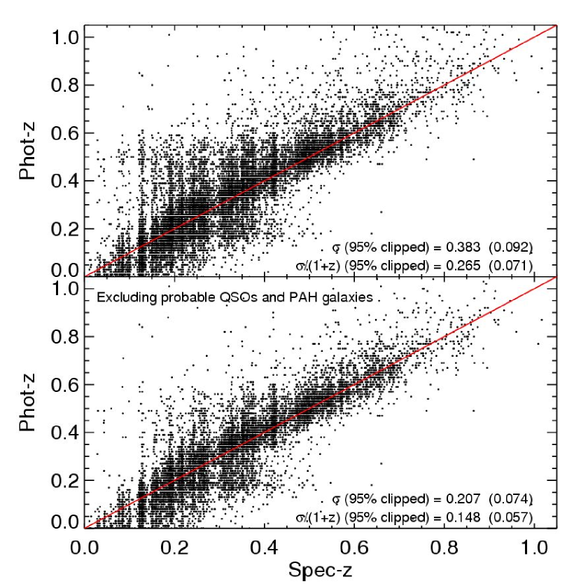
Figure 1.— Comparison of calibrated template–fitting photometric redshifts with AGES spectroscopy. In the top panel all $z<1.1$ AGES objects are plotted, whereas in the bottom panel likely AGN and strongly PAH–emitting galaxies have been removed. The full rms dispersion markedly improves in the bottom panel. The clipped statistics (in parentheses) are quite good in both cases, with $\sigma\lesssim 0.1$.

As discussed above, PAH–emitting and active galaxies, two object classes not represented in the empirical galaxy templates, are over–represented in the AGES sample. To see how this affects the statistics, the lower panel of Figure 1 omits objects likely to be either PAH–emitters or AGN. The former are defined in this work as objects with an IRAC color of $[5.8]-[8.0]>1$. The latter were identified on the basis of their infrared colors in an IRAC color–color diagram similar to the one described in detail in Stern et al. (2005). That paper demonstrated that active galaxies can be readily identified based solely on their infrared colors (also see Lacy et al., 2004). Omitting these two populations removes 70% of the variance, or about half the rms error, while maintaining similar clipped statistics. We now turn to techniques of estimating redshifts for these populations.

3.3. Artificial Neural Net Algorithm

Although the utility of purely empirical methods is limited to the parameter space of the calibration sample, such methods do offer several unique advantages. Neither absolute band–to–band calibrations, nor a complete knowledge of the galaxy population are required for accurate redshift estimation. Given a large spectroscopic training set, algorithms such as polynomial fits or artificial neural nets (ANNs) can be trained to predict the redshifts of objects of all types using the actual survey photometry.

Regardless of method, the uniqueness of the mapping from colors to redshifts is the underlying limitation in redshift accuracy. Objects with approximately power–law spectra such as QSOs will never allow very accurate photometric redshift estimation. Nevertheless, empirical methods do in principle allow the best redshift estimation possible for each population. For populations with strong spectral features but lacking accurate template spectra, empirical algorithms are expected to show marked improvement over template–fitting methods.

To improve the redshift estimation of $z<0.5$ PAH–emitting starburst galaxies, as well as very active galaxies, for which the AGN component dominates the observed mid–IR emission, the AGES spectroscopic sample was used to train a neural net algorithm. We adopted the public code ANNz (Collister and Lahav, 2004) for this purpose.

Briefly, the ANN is trained to match a set of observational inputs (in this case galaxy photometry) to a set of known outputs (the spectroscopic redshifts) by minimizing a cost function. The form of the cost function is determined by the architecture of the ANN, which specifies the number of hidden nodes between the input and output nodes. Following Firth et al. (2003), we employ a 7:10:10:10:1 architecture, which takes 7 inputs, the $B_{W}RI[3.6][4.5][5.8][8.0]$ photometry, has three 10–node hidden layers and a single output node, the photometric redshift (see Collister and Lahav, 2004; Firth et al., 2003; Lahav et al., 1996, for details). The inclusion of the $[5.8]$ and $[8.0]$ photometry (or limits) allow the PAH features in starburst galaxies and the mid–IR excesses in active galaxies to be fitted, or at least differentiated. Only objects observed in all of the above bands were used in the fit; the near–IR data covering only a subset of the field was not used.

The AGES sample was divided into training, validation and testing subsets, containing 7500, 2500, and 5052 objects, respectively. The cost function is fitted on the training set and evaluated on the validation set after each iteration. When trained, the algorithm can be run on the independent testing set to determine the accuracy of the method. The “consensus” median prediction from a committee of ANNs, each the result of independent training sessions (initialized with different random seeds), produces the most reliable redshifts and error estimates (e.g., Firth et al., 2003). Although the current implementation of ANNz does not incorporate the photometric errors in its determination of the photometric redshift, it does use them to estimate the redshift uncertainties. A committee of 10 ANNs was adopted in this work.

The results are plotted in Figure 2 for both the full AGES sample (top panel), and the smaller test set which was independent of the ANN training. The results for these two samples are essentially identical, indicating that our training sample is large enough to span the distribution of spectral types and redshifts in the AGES sample. The dispersion over all redshifts, $\sigma\sim 0.13$, is dominated by the $z>1$ AGN, whose weak broad–band spectral features lead to greater redshift uncertainty for any algorithm. Considering just the $z<1$ AGES galaxies, we find the dispersion drops to $\sigma\sim 0.08$, whereas for the $z>1$ AGN it rises to $\sigma\sim 0.4$. This is typical of the accuracy of other attempts to measure AGN redshifts photometrically (e.g., Kitsionas et al., 2005; Babbedge et al., 2004; Weinstein et al., 2004).

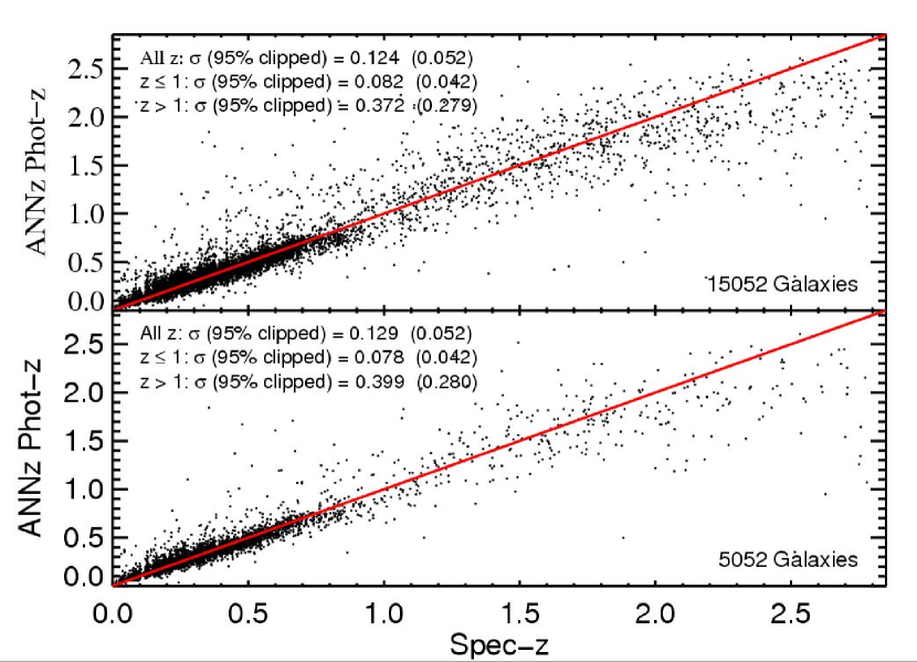
Figure 2.— ANNz photometric vs. spectroscopic redshift for the full AGES sample (top panel), and the testing sample alone (bottom). The clipped results are quite similar in both samples, with very accurate ($\sigma\sim 0.05$) redshift prediction for the normal galaxy sample at $z<1$ (including PAH–emitting galaxies), and more modest accuracy ($\sigma\sim 0.3-0.4$) at $z>1$ where the sample is dominated by QSOs and AGN.

3.4. Hybrid Approach

In assessing the advantages and drawbacks of the two redshift algorithms presented so far, an obvious complementarity is apparent. The ANN provides excellent redshift estimation for low–z galaxies bright enough to have well measured photometry in all 4 IRAC bands, including strongly PAH–emitting galaxies. Furthermore, the ANN redshift accuracy for AGN is superior at all redshifts to that achievable by template–fitting methods. Due to the IR–excess of these active galaxies (Stern et al., 2005), large numbers of them are well-measured in all four IRAC bands, at least out to $z\sim 2$. Therefore, within the bright limits of the AGES survey, these two populations are well represented and hence well calibrated in the ANN.

The template–fitting method, while not reliable for accretion–dominated active galaxies, is quite robust for normal galaxies in the $z\lesssim 1$ AGES sample, barring low redshift strong PAH–emitters. This method has the critical advantage that it is expected to be robust outside the parameter space in which it was tested. In particular it should be reliable to magnitudes much fainter that the AGES sample, and out to higher redshift. Another important advantage of this method is that it allows straightforward generation of redshift probability functions, which are essential for many applications. Finally, it produces restframe properties for the fitted galaxies, such as absolute magnitudes.

We therefore construct a hybrid photometric redshift sample, combining the above methods according to their strengths. While it is tempting to simply adopt the ANN method for all bright galaxies, we limit its sphere of influence to the color–selected AGN and PAH–emitters as defined below.

Selection of objects for ANN redshift estimation was made using color cuts in $[3.6]-[4.5]$ vs. $[5.8]-[8.0]$ color–color space, illustrated in Figure 3. Model tracks illustrate where representative quiescent and starburst galaxies appear from $0\leq z\leq 2$ in this plot. Objects lying in the “AGN wedge”, defined in Stern et al. (2005), were classified as likely active galaxies. On the other hand, objects outside the AGN wedge and with $[5.8]-[8.0]>1$ were taken to be potential PAH galaxies. For both populations we only estimated redshifts for objects matching the IRAC flux limits of the full spectroscopic sample, which were $[17.5,17.0,16.2,15.5]$ for AGN and $[16.75,16.6,16.2,14.25]$ for PAH–emitters in the 3.6, 4.5, 5.8, and 8.0 micron bands, respectively. The limits are generally deeper for the active galaxies since unresolved AGN candidates were targeted to a greater depth in AGES. No extrapolation to fainter magnitudes was allowed for either object class. In addition, adequate photometric coverage was required in all 7 bands that were used in the calibration of the ANN.

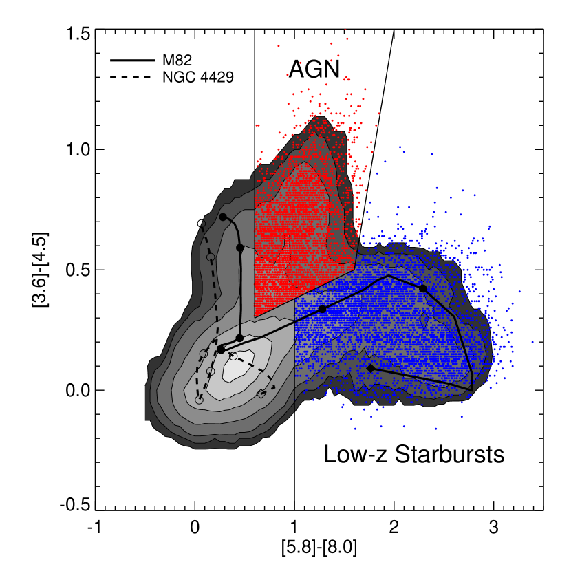
Figure 3.— IRAC color–color plot showing the color criteria for inclusion in the neural net component of the hybrid photometric redshift algorithm. Grey contours illustrate the colors of the full photometric redshift sample. The likely AGN and PAH-emitters are overplotted in red and blue points, respectively. In addition to these color selections, objects are subject to strict AGES–defined flux limits, as defined in the text. Model tracks of two $0\leq z\leq 2$ non–evolving galaxy templates from Devriendt et al. (1999) are also plotted. The solid curve represents M82, a starburst galaxy; the dashed curve shows NGC 4429, an S0/Sa galaxy with a star formation rate approximately 4000 times lower. The tracks begin at $z=0$ at the diamond symbols, and circular annotations are made at z = 0.25, 0.5, 0.75, 1.0, 1.5, and 2.0.

The strong flux constraints, in particular in the $[5.8]$ and $[8.0]$ bands, limit the sample to the very brightest AGN at $z\lesssim 2.5$ and PAH–emitters at $z\lesssim 0.5$, as in the AGES sample. The final selection included 3681 AGN and 4766 PAH–emitters for which the template–fitting redshifts were replaced with ANN redshifts. Representing only $\sim 4\%$ of the galaxy sample, this approach serves primarily to reduce the number of outliers.

3.5. Comparison to Spectroscopy

In this Section we demonstrate that the hybrid method surpasses the simple template–fitting algorithm in redshift accuracy for both galaxies and AGN, though the improvement is more substantial for the latter. We adopt the QSO/AGN targeting criteria employed in the AGES survey to distinguish between normal and active galaxies. These criteria, described fully in Kochanek et al. (in preparation), identify AGN by combining optical morphology with flux or color cuts in x–ray through radio wavelengths.

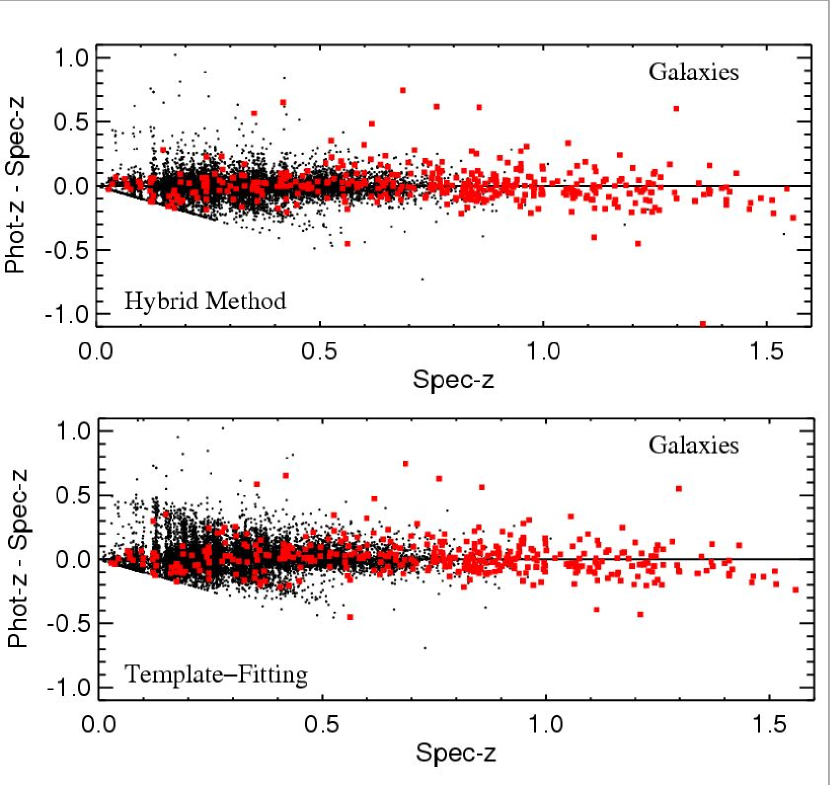
Figure 4.— Hybrid (top) and template–fitting (bottom) photometric redshifts for the AGES galaxy sample (dots) and the deeper, in–house spectroscopic sample (filled squares). The hybrid method produces a major improvement in $z\lesssim 0.5$ starburst galaxies, and, as quantified in Table 1, reduces the overall dispersion by over 20% compared with the standard template–fitting method.

Figure 4 compares the hybrid (top panel) and template–fitting (bottom panel) photometric redshift predictions to the spectroscopy for the AGES sample of galaxies (dots). The difference between the methods is subtle, but most evident at low redshift ($z\sim 0.2$) where the improvement for starburst PAH–emitters is apparent. Also plotted is the in–house spectroscopic galaxy sample (filled squares), which extends to much fainter flux limits ($R\sim 25$) and higher redshifts than the AGES galaxies. As such it provides a valuable, independent test of the method. Clearly redshift estimation is reliable to $z\sim 1.5$ for this deeper sample. There are a handful of outliers between $0.5\lesssim z\lesssim 1$, and evidence of possible systematic errors at $z\lesssim 0.25$ where the $B_{W}$ filter is not fully blueward of the 4000 Å break.

Various measures of the accuracy of the hybrid and template–fitting methods are given in Table 1. The basic result is that a redshift accuracy of $\sigma\approx 0.06\,(1+z)$ is being achieved for 99.5% of galaxies in the AGES sample. For the more challenging in–house sample, 98.5% of galaxies have a redshift accuracy of $\sigma\approx 0.10\,(1+z)$. The hybrid method also reduces the number of outliers, as seen in the fraction of 3$\sigma$ outliers. The final two columns of Table 1 report the dispersions for subsamples constrained to contain 95% of the objects, thereby allowing a direct comparison of the hybrid and template methods. Clearly the hybrid method is superior, reducing the dispersion by over 20% compared with standard template-fitting.

Table 1Photometric Redshift Accuracy for Galaxies

			Unclipped			3$\sigma$ Clipped				95% Clipped
Sample	Algorithm		$\sigma$	$\sigma/(1+z)$		% Rejected	$\sigma$	$\sigma/(1+z)$		$\sigma$	$\sigma/(1+z)$
AGES	Hybrid		0.143	0.105		0.52	0.077	0.060		0.060	0.047
In–House	Hybrid		0.397	0.185		1.46	0.160	0.096		0.101	0.059
AGES + In–House	Hybrid		0.160	0.109		0.53	0.080	0.061		0.062	0.048
AGES	Template		0.230	0.170		0.60	0.102	0.081		0.079	0.061
In–House	Template		0.498	0.253		2.51	0.190	0.111		0.127	0.081
AGES + In–House	Template		0.245	0.174		0.69	0.104	0.082		0.081	0.062

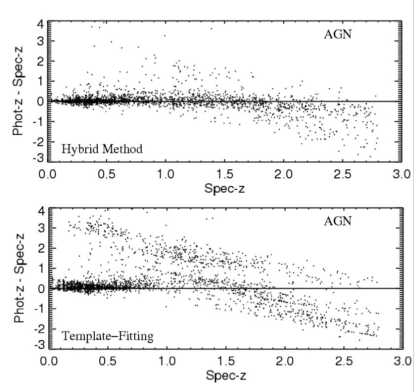
Figure 5.— Hybrid (top panel) and template–fitting (bottom panel) photometric redshifts for the AGN sample. The improvement of the hybrid method is clear at all redshifts, dramatically so at $z>1$. A statistical comparison of the two methods, given in Table 2, demonstrates that the hybrid method reduces the redshift dispersion by 65% over the template–fitting method.

Figure 5 shows a similar comparison for the AGN sample. Here the improvement of the hybrid technique over simple template–fitting is dramatic, though not surprising. With no AGN template in the mix, the template–fitting algorithm should not be expected to succeed for accretion–dominated objects. This is clear from the lower panel of this figure, where beyond $z\gtrsim 1$ the results are essentially useless. The fairly accurate results at low redshift are likely for galaxies which, though active, have luminosities dominated by fusion processes. In the bright AGES sample, these galaxies would only be visible at modest redshifts, whereas the $z>1$ sample should be almost entirely composed of extremely luminous quasars (some of which are also present at low redshift).

As a check on this hypothesis, histograms of the morphological stellarity indicator discussed above are plotted in Figure 6 for two AGN subsets, split according to their observed redshift accuracy and range. Those AGN for which the template–fitting algorithm works reasonably well, taken to be those with both spectroscopic redshifts and absolute redshift differences of less than unity, are plotted as the solid histogram in Figure 6. The complement, for which the algorithm largely fails, is plotted as a dot–dashed histogram. Thus the bimodality observed in the lower panel of Figure 5 is strongly reproduced in the morphological stellarity measurements in Figure 6. The AGN for which the template–fitting method works are clearly resolved objects for which the nuclear emission does not dominate the flux of the galaxy. Conversely, the redshift failures are overwhelmingly unresolved sources, consistent with the expectation of nuclear–dominated emission from very luminous AGN and QSOs.

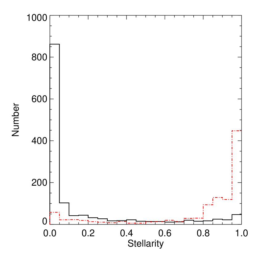
Figure 6.— Histogram of the SExtractor CLASS_STAR parameter in the best-seeing optical band of two subsets of AGN isolated from the lower panel of Figure 5. This parameter varies continuously between zero and unity, where the extreme values correspond to sources which are completely resolved and unresolved, respectively. The solid histogram represents those objects for which the template–fitting algorithm is reasonably robust, taken to be those objects with $|\mbox{Phot--}z-\mbox{Spec--}z|<1$ and $\mbox{Spec--}z<1$. The dot–dashed histogram is for those objects excluded by this selection. Clearly the template-fitting algorithm works well for resolved AGN and fails for truly quasi–stellar objects.

In marked contrast with the template-fitting redshifts, the hybrid redshifts (top panel of Figure 5) are quite accurate for all AGN to $z\sim 2$, with no obvious systematic issues or significant occurrence of catastrophic errors. Beyond $z>2$ the redshifts for AGN are systematically underestimated, presumably due the relative paucity of calibrators at these high redshifts.

Statistics of the redshift accuracy for AGN are given in Table 2. The hybrid redshift dispersion is $\sigma\approx 0.14\,(1+z)$ for over 97% of the active galaxies. The tremendous improvement achieved by this method, apparent in Figure 5, is borne out in a direct statistical comparison of the 95%–clipped samples. The dispersion of the hybrid method is a factor of 3 smaller than that achieved with galaxy template fitting.

Table 2Photometric Redshift Accuracy for AGN

			Unclipped			3$\sigma$ Clipped				95% Clipped
Sample	Algorithm		$\sigma$	$\sigma/(1+z)$		% Rejected	$\sigma$	$\sigma/(1+z)$		$\sigma$	$\sigma/(1+z)$
AGES	Hybrid		0.473	0.219		2.94	0.309	0.138		0.255	0.120
AGES	Template		0.998	0.540		0.60	0.918	0.462		0.797	0.341

3.6. Comparison with an Independent Photometric Redshift Catalog

We have also verified that the hybrid photometric redshift algorithm presented here is in excellent agreement with an independent photometric redshift catalog in the same field. Brown et al. (in preparation), adopting a pure neural net approach, have generated a photometric redshift catalog from independently extracted multi–color catalogs, photometered with an original code. By making fainter copies of the AGES spectroscopic galaxies, they have effectively extended the calibration set to much fainter magnitudes. In addition to the photometric data, structural information, in the form of sizes of the major and minor axes, was also incorporated into the neural net for bright objects to improve accuracy at low redshift. Using an independent calibration of the neural net on this extended sample, they derive neural net photometric redshifts for a large optically-selected sample in Boötes.

At relatively bright magnitudes ($R\leq 23$) objects with SExtractor CLASS_STAR parameters greater than 0.85, measured in the best–seeing optical band, are taken be stars (Jannuzi et al. in preparation) and are removed for this comparison. The stellar contamination is negligible faintward of this limit and no attempt is made to remove fainter stars. Over the redshift range where spectroscopic calibrators exist, $0<z\lesssim 1.5$, the inter–catalog 95% clipped redshift dispersion for the sample of galaxies common to both samples is $\sigma=0.09$, or $\sigma=0.05\,(1+z)$. These two sets of redshifts were computed using independent galaxy photometry and error estimates, and for the vast majority of objects, different photometric redshift algorithms (template–fitting vs. artificial neural net). Yet there is excellent agreement, similar in accuracy to that demonstrated versus spectroscopy in the preceding section, probing right down to the 13.3$\mu$Jy limit. This provides strong evidence that both photometric redshift catalogs are free from substantial systematic errors.

3.7. Dependence on Magnitude and SED

Comparing the results for the AGES and in-house galaxy samples in Table 1, it is clear that the redshift precision is lower for the fainter in-house sample. In general the photometric redshift precision depends on both photometric S/N and galaxy spectral type, with slightly smaller uncertainties typically achieved for redder galaxies due to their larger continuum breaks. Table 3 quantifies the hybrid redshift accuracy in differential magnitude bins for galaxies classified in the template fits as earlier or later than an unevolved CWW Sbc galaxy.

Table 3Dependence on Galaxy Magnitude and SED

		Early–Type			Late–Type
4.5$\mu$m Mag Range		$\sigma$	$\sigma/(1+z)$		$\sigma$	$\sigma/(1+z)$
14.5 – 15.0		0.039	0.031		0.038	0.030
15.0 – 15.5		0.038	0.029		0.046	0.034
15.5 – 16.0		0.040	0.029		0.049	0.036
16.0 – 16.5		0.050	0.037		0.071	0.054
16.5 – 17.0		0.069	0.054		0.083	0.063
17.0 – 17.5		0.074	0.060		0.073	0.057

Note. — The AGES + in–house galaxy sample is divided into early– and late–type samples according to the best–fit SED templates; objects with best-fit templates earlier than an unevolved CWW Sbc template are classified as early–type, whereas those of type Sbc or later are taken to be late–type. Statistics are for the 95% clipped sample.

The available spectroscopy beyond the AGES 4.5$\mu$m statistical limit of 15.7 mag is both incomplete and inhomogeneous. The tabulated redshift accuracies therefore may not be representative of those which would be obtained for magnitude limited samples to fainter depths.

4. Redshift Probability Functions

Redshift likelihood functions were constructed by projecting the likelihood surface of redshift and spectral type onto the redshift axis. Convolution of these likelihood functions with a variable–width Gaussian kernel, which increases the error with redshift, accounts for the template–mismatch variance inherent in the method (e.g., Brodwin et al., 2006; Fernandez-Soto et al., 2002). From the results of Table 1, the kernel is taken to be $\sigma(z)=0.06(1+z)$.

This renders the area under these functions reasonable proxies of redshift probability density, resulting in approximate redshift probability distribution functions (PDFs) for all objects in the survey. Due to the excellent redshift accuracy for $0<z<1.5$, no redshift prior was applied to these likelihood functions, other than the weak prior imposed by the limited fitting range. Stronger priors can, of course, be imposed for certain kinds of analyses; we employ this methodology in computing the galaxy redshift distribution in the next section. The statistical validity of the PDFs in the present paper can be explicitly confirmed for those objects which have spectroscopic redshifts as follows.

Redshift confidence intervals are derived from the PDFs by associating area with probability density as illustrated in Figure 7. We define the 1$\sigma$, 2$\sigma$, and 3$\sigma$ confidence intervals as those redshift regions which enclose the top 68.3%, 95.4% and 99.7% of the normalized area under the PDFs.

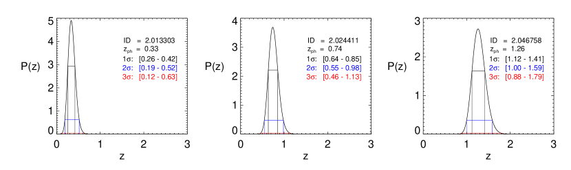
Figure 7.— Redshift PDFs for 3 sample galaxies, with the 1$\sigma$ (68.3%), 2$\sigma$ (95.4%), and 3$\sigma$ (99.7%) confidence intervals denoted by horizontal lines under the curves.

While the full PDF should in general be used for statistical analyses of the galaxy population, confidence intervals defined in this way offer a straightforward test of the PDFs. In Table 4 we report the fraction of objects which agree with the spectroscopic redshift at each confidence level, for both the full spectroscopic sample and for the galaxy sample alone (i.e., excluding objects identified as QSOs and AGN in AGES, but including PAH–emitting starburst galaxies). We only consider objects here with photometry of sufficient quality to be included in the main photometric redshift sample as described in Section 2.2.2.

The $1\sigma$ confidence intervals are approximately Gaussian for the full sample in that the spectroscopic redshift is included in this photometric redshift confidence interval for 70% of the objects. The 2$\sigma$ and 3$\sigma$ confidence intervals have inclusion rates slightly below the Gaussian expectation, by 3.9% and 2.7%, respectively. This small outlier fraction is reduced to 0.8% and 1.2% when QSOs and AGN are excluded, though the $1\sigma$ interval is slightly conservative in this case. That the inclusion of a large fraction of active galaxies affects the statistics so little is an indication of the robustness of the redshift probability functions. The lack of strong continuum spectral features results in quite broad redshift probability functions for these objects, reflective of the larger uncertainty in their redshifts. These lead to wide, but valid, confidence intervals, which can be incorporated in large statistical studies. On the other hand, previous IRAC Shallow survey papers (Eisenhardt et al., 2004; Stern et al., 2005) have demonstrated how these objects can be reliably removed, if desired, using photometric information prior to redshift fitting.

Table 4Confidence Level Statistics

		All Objects			Galaxies
Confidence	Gaussian	Correct Within	Observed		Correct Within	Observed
Level	Expectation	Confidence Interval	Fraction		Confidence Interval	Fraction
$\leq 1\sigma$	68.3%	10870/15530	70.0%		9722/13043	74.5%
$\leq 2\sigma$	95.4%	14206/15530	91.5%		12335/13043	94.6%
$\leq 3\sigma$	99.7%	15065/15530	97.0%		12848/13043	98.5%
$>3\sigma$	0.3%	465/15530	3.0%		195/13043	1.5 %

5. Science Applications

A shared primary goal of the IRAC Shallow, NDWFS and FLAMEX surveys is to study structure formation and evolution at $0.5<z<2$, both in the field and in cluster environments. In this Section we present two specific large scale structure science applications enabled by the hybrid photometric redshifts and redshift probability distributions derived in this paper: a measurement of the 4.5$\mu$m galaxy redshift distribution, and the discovery of a high–redshift ($z>1$) galaxy cluster.

5.1. Redshift Distribution at 4.5$\mu$m

A key issue in structure formation models is the mass assembly history of massive galaxies (e.g., Faber et al., 2006). Recent work (Yan et al., 2005; Mobasher et al., 2005; Bunker et al., 2006) has indicated that massive galaxies form the bulk of their stars soon after reionization, and evolve passively over most of the history of the universe (Treu et al., 2005; Juneau et al., 2005; Bundy et al., 2005). While hierarchical models can accommodate a modest number of early, massive halos, these results were not predicted in advance of the observations.

More generally, any viable galaxy formation theory must predict the low order moments of the mass distribution, including the redshift distribution and the autocorrelation function. Previous attempts to constrain galaxy formation models using these moments have been limited by the difficulty in relating optical light to mass, the natural theoretical variable. Kauffmann and Charlot (1998) suggested employing a $K$–band selection to minimize this source of uncertainty, and Cimatti et al. (2002, hereafter K20) subsequently presented the $K_{s}<20$ redshift distribution. Their sample had a median redshift of $z_{\mbox{\small{med}}}\sim 0.80$, and a distribution that was best reproduced by pure luminosity evolution models.

However, the $K$–band is only a good proxy for stellar mass at redshifts where it samples the rest–frame near-IR stellar peak. At $1<z<2$, where significant elliptical galaxy assembly is expected in hierarchical models (e.g., Kauffmann, 1996), the stellar peak is firmly in the Spitzer/IRAC bands. We therefore present in Figure 8 the 4.5$\mu$m galaxy redshift distribution derived from the 13.3$\mu$Jy sample described above. The survey is over 85% complete to this limit, based on the recovery fraction of artificial stars in standard completeness simulations. Very strict multi–band masking was employed in determining the redshift distribution, rejecting areas not containing valid coverage in all of the key optical ($B_{W}RI$) and IRAC ($[3.6][4.5]$) bands. This resulted in a final unmasked area of 7.25 deg². Stars are rejected at bright magnitudes only, using the criteria described in §3.6.

Figure 8.— Differential 4.5$\mu$m–selected photometric redshift distribution in Boötes. The hybrid redshift catalog was used for the histogram. The smooth curve was constructed from summing up the individual galaxy redshift probability functions as described in the text. The dashed vertical line indicates the maximum redshift at which the photometric redshift method has been verified against spectroscopy.

The redshift distribution is calculated in two ways. The simple histogram is derived using the best-estimate redshifts of the hybrid method. The curve in the figure shows the result of summing up the full normalized redshift probability function for each galaxy, following the method of Brodwin et al. (2006). The prior in this method is taken to be the approximate $N(z)$ estimated from a direct summation of the galaxy likelihood functions. The vertical dashed line represents the redshift limit of the available spectroscopy; beyond this limit the robustness of the photometric redshifts has not been explicitly demonstrated. The median redshift is $z_{\mbox{\small{med}}}=0.98$ for the simple hybrid–method histogram, and $z_{\mbox{\small{med}}}=0.99$ for the PDF summation method. Assuming the galaxies with formal photometric redshifts of $z\geq 2$ are distributed according to the plotted $0<z<2$ distribution, the median redshifts are $z_{\mbox{\small{med}}}=0.85$ and $z_{\mbox{\small{med}}}=0.88$, respectively. The two methods are in excellent agreement, which, while not tautological, is nevertheless expected. It provides a measure of confidence in the consistency of the methods employed here.

Despite being shallower than the K20 survey, the IRAC Shallow survey has a higher median redshift, owing to a beneficial, negative K–correction (e.g., Eisenhardt et al. in preparation). This deeper reach, along with a 500–fold increase in area over the K20 survey, enables stronger constraints to be placed on models of galaxy evolution. We will be examining this in detail in a future paper.

5.2. A High Redshift Galaxy Cluster Search

We present some early results of a high redshift ($z>1$) galaxy cluster search underway in the Boötes field. The detection technique, described in Eisenhardt et al. (in preparation, see also Stanford et al. 2005; Elston et al. 2006; Gonzalez et al. in preparation), implements a wavelet search algorithm tuned to identify structure on cluster scales ($\sim 500$ kpc). The redshift probability functions are the input to the wavelet code, and so the cluster detection is principally dependent on the accuracy and statistical reliability of the redshift PDFs. The method is independent of the strength, or even presence, of the cluster red sequence, and therefore provides an unbiased window on the era of cluster formation.

Four cluster candidates were targeted spectroscopically in the first half of 2005, and all four were confirmed to be $z>1$ galaxy clusters, at redshifts ranging from $\left<z\right>=1.11$ to $\left<z\right>=1.41$. The latter cluster, the highest yet found in a cluster survey, is presented in Stanford et al. (2005). In this Section we present one of the newly discovered clusters, a filamentary cluster at $\left<z\right>=1.24.$

The cluster ISCS J1434.5+3427 is shown in Figure 9. The cluster–finding power of the Spitzer/IRAC imaging is clearly demonstrated in this figure. Though no structure is apparent in the optical bands, a striking filamentary structure emerges beyond rest–frame 4000 Å in the 4.5$\mu$m band. The spectroscopic cluster members are circled in red on the greyscale 4.5$\mu$m image. Objects which have the cluster systemic redshift of $\left<z\right>=1.24$ within their 1$\sigma$ confidence intervals are marked by blue squares.

ISCS J1434.5+3427 was observed spectroscopically in 2005 February with Keck/LRIS (Oke et al., 1995) and 2005 May with Keck/DEIMOS (Faber et al., 2003). For a more detailed description of these spectroscopic observation see Stanford et al. (2005) and Desai et al. (in preparation). The eight spectroscopic members within $\Delta z=0.01$ of the systemic redshift confirm the reality of this cluster at $\left<z\right>=1.241$. Details of these members are given in Table 5. An estimate of the cluster velocity dispersion is deferred until additional spectroscopy yields more members. In addition, deep follow–up imaging observations with HST/ACS and Spitzer/IRAC are underway.

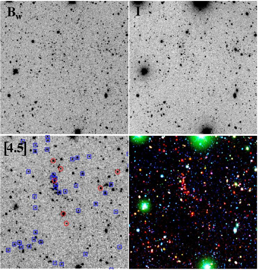
Figure 9.— 5′$\times$5′ $B_{W}$, $I$, $[4.5]$, and composite color image of cluster ISCS J1434.5+3427 at $\left<z\right>=1.24$. North is up and East is left. Notice the striking filamentary morphology that emerges in the 4.5$\mu$m band, and is quite prominent in the composite image. Spectroscopically confirmed cluster members are denoted by red circles on the $[4.5]$ image. Objects which contain the cluster systemic redshift within their 1$\sigma$ photometric redshift confidence levels are denoted with blue squares.

Table 5Summary of Spectroscopic Members

					95% Confidence
ID	R.A.	Dec.	$[4.5]$	phot–$z$	Interval	spec–$z$	$\delta z$	Date	Instrument
IRAC J143430.3+342712	14:34:30.36	+34:27:12.1	15.81	1.26	[0.98, 1.63]	1.2365	0.0005	UT 2005 Feb 10	LRIS
IRAC J143428.6+342557	14:34:28.66	+34:25:57.7	15.19	1.12	[0.89, 1.43]	1.238	0.003	UT 2005 Feb 10	LRIS
IRAC J143421.6+342656	14:34:21.64	+34:26:56.2	16.67	1.09	[0.84, 1.37]	1.2502	0.0005	UT 2005 Feb 11	LRIS
IRAC J143429.2+342739	14:34:29.21	+34:27:39.1	16.99	1.06	[0.68, 1.49]	1.2436	0.0005	UT 2005 Feb 11	LRIS
IRAC J143430.1+342657	14:34:30.15	+34:26:57.2	15.90	1.17	[0.92, 1.48]	1.23	0.01	UT 2005 Feb 11	LRIS
IRAC J143428.0+342535	14:34:28.05	+34:25:35.8	16.64	1.19	[0.89, 1.57]	1.240	0.002	UT 2005 May 07	DEIMOS
IRAC J143418.4+342733	14:34:18.41	+34:27:33.1	16.42	1.21	[0.96, 1.52]	1.240	0.001	UT 2005 May 07	DEIMOS
IRAC J143430.6+342757	14:34:30.63	+34:27:57.2	15.35	0.95	[0.00, 4.17]	1.242	0.002	UT 2005 May 07	DEIMOS

6. Summary

Accurate photometric redshifts, calibrated using over 15,000 spectroscopic redshifts, have been computed for a 4.5$\mu$m sample of 194,466 galaxies in the 8.5 deg² IRAC Shallow survey. A hybrid technique, in which a standard template fitting code is augmented using a neural net approach, was adopted to optimize the redshift accuracy for both active and low–$z$ starburst galaxies without compromising reliability for the general galaxy population. This is primarily enabled by the fact that these two populations, which are often troublesome for template-fitting codes, are particularly well represented in the AGES sample. Between $0<z<1.5$ the resulting hybrid algorithm has a demonstrated accuracy of $\sigma\lesssim 0.06\,(1+z)$ for 95%, and $\sigma\lesssim 0.1\,(1+z)$ for 98.5%, of the galaxy population. For over 97% of the active galaxies, the redshift accuracy is $\sigma\lesssim 0.14\,(1+z)$.

Redshift probability functions have been computed for all objects directly from the template–fitting algorithm. Comparison with the large spectroscopic sample has verified the statistical validity of these functions, and in particular, the reliability of confidence intervals derived from them. These confidence intervals, or indeed the full probability functions, can be reliably used in statistical studies of the galaxy population. Several such programs are underway, and we present in this paper two new results which employ them.

The 4.5$\mu$m-selected galaxy redshift distribution, a primary observable for confronting theories of structure formation, was computed using both the hybrid photometric redshifts and the full redshift probability functions. The methods yield entirely consistent results. This measurement is provided in anticipation of future model predictions extending into the mid–IR, where flux is closely related to stellar mass above $z\gtrsim 1$.

Another program making extensive use of these redshift PDFs is a search for high redshift ($z>1$) galaxy clusters. We presented one such cluster, ISCS J1434.5+3427, spectroscopically confirmed at $\left<z\right>=1.24$, which was discovered by incorporating the redshift PDFs in a wavelet search algorithm. Spectroscopic confirmations of two similarly discovered high redshift clusters, at $\left<z\right>=1.11$ and $\left<z\right>=1.41$, are presented in companion papers (Stanford et al., 2005; Elston et al., 2006). A complete description of the cluster survey sample and methodology is presented in Eisenhardt et al. (in preparation), along with the spectroscopic confirmation of a $\left<z\right>=1.37$ cluster.

References

- Babbedge et al. (2004) Babbedge, T. S. R., et al. 2004, MNRAS, 353, 654
- Benítez (2000) Benítez, N. 2000, ApJ, 536, 571
- Bertin and Arnouts (1996) Bertin, E. and Arnouts, S. 1996, A&AS, 117, 393
- Blake et al. (2006) Blake, C., Collister, A., Bridle, S., and Lahav, O. 2006, ArXiv Astrophysics e-prints MNRASsubmitted (astro–ph/0605303)
- Brand et al. (2006) Brand, K., et al. 2006, ApJ, in press (astro–ph/0512343)
- Brodwin et al. (2006) Brodwin, M., Lilly, S. J., Porciani, C., McCracken, H. J., Le Fèvre, O., Foucaud, S., Crampton, D., and Mellier, Y. 2006, ApJS, 162, 20
- Brunner et al. (2000) Brunner, R. J., Szalay, A. S., and Connolly, A. J. 2000, ApJ, 541, 527
- Bruzual and Charlot (2003) Bruzual, G. and Charlot, S. 2003, MNRAS, 344, 1000
- Bundy et al. (2005) Bundy, K., Ellis, R. S., and Conselice, C. J. 2005, ApJ, 625, 621
- Bunker et al. (2006) Bunker, A., Stanway, E., Ellis, R., McMahon, R., Eyles, L., and Lacy, M. 2006, New Astronomy Review 50, 94
- Cimatti et al. (2002) Cimatti, A., et al. 2002, A&A, 391, L1
- Collister and Lahav (2004) Collister, A. A. and Lahav, O. 2004, PASP, 116, 345
- Connolly et al. (1995) Connolly, A. J., Csabai, I., Szalay, A. S., Koo, D. C., Kron, R. G., and Munn, J. A. 1995, AJ, 110, 2655
- Connolly et al. (1997) Connolly, A. J., Szalay, A. S., Dickinson, M., Subbarao, M. U., and Brunner, R. J. 1997, ApJ, 486, L11
- Cool et al. (2006) Cool, R. J., et al. 2006, ApJ, in press (astro–ph/0605030)
- Devriendt et al. (1999) Devriendt, J. E. G., Guiderdoni, B., and Sadat, R. 1999, A&A, 350, 381
- Eisenhardt et al. (2004) Eisenhardt, P. R., et al. 2004, ApJS, 154, 48
- Elston et al. (2006) Elston, R. J., et al. 2006, ApJ, 639, 816
- Faber et al. (2003) Faber, S. M., et al. 2003, in Instrument Design and Performance for Optical/Infrared Ground-based Telescopes. Edited by Iye, Masanori; Moorwood, Alan F. M. Proceedings of the SPIE, Volume 4841, pp. 1657-1669 (2003)., pp 1657–1669
- Faber et al. (2006) Faber, S. M., et al. 2006, ApJ, submitted (astro–ph/0506044)
- Fabricant et al. (2005) Fabricant, D., et al. 2005, PASP, 117, 1411
- Fernandez-Soto et al. (2002) Fernandez-Soto, A., Lanzetta, K. M., Chen, H.-W., Levine, B., and Yahata, N. 2002, MNRAS, 330, 889
- Fioc and Rocca-Volmerange (1999) Fioc, M. and Rocca-Volmerange, B. 1999, ArXiv Astrophysics e-prints
- Firth et al. (2003) Firth, A. E., Lahav, O., and Somerville, R. S. 2003, MNRAS, 339, 1195
- Firth et al. (2002) Firth, A. E., et al. 2002, MNRAS, 332, 617
- Fontana et al. (2000) Fontana, A., D’Odorico, S., Poli, F., Giallongo, E., Arnouts, S., Cristiani, S., Moorwood, A., and Saracco, P. 2000, AJ, 120, 220
- Helou et al. (2000) Helou, G., Lu, N. Y., Werner, M. W., Malhotra, S., and Silbermann, N. 2000, ApJ, 532, L21
- Hsieh et al. (2005) Hsieh, B. C., Yee, H. K. C., Lin, H., and Gladders, M. D. 2005, ApJS, 158, 161
- Jannuzi and Dey (1999) Jannuzi, B. T. and Dey, A. 1999, in ASP Conf. Ser. 191 — Photometric Redshifts and the Detection of High Redshift Galaxies, p. 111
- Juneau et al. (2005) Juneau, S., et al. 2005, ApJ, 619, L135
- Kauffmann (1996) Kauffmann, G. 1996, MNRAS, 281, 487
- Kauffmann and Charlot (1998) Kauffmann, G. and Charlot, S. 1998, MNRAS, 297, L23+
- Kenter et al. (2005) Kenter, A., et al. 2005, ApJS, 161, 9
- Kinney et al. (1996) Kinney, A. L., Calzetti, D., Bohlin, R. C., McQuade, K., Storchi–Bergmann, T., and Schmitt, H. R. 1996, ApJ, 467, 38
- Kitsionas et al. (2005) Kitsionas, S., Hatziminaoglou, E., Georgakakis, A., and Georgantopoulos, I. 2005, A&A, 434, 475
- Lacy et al. (2004) Lacy, M., et al. 2004, ApJS, 154, 166
- Lahav et al. (1996) Lahav, O., Naim, A., Sodré, L., and Storrie-Lombardi, M. C. 1996, MNRAS, 283, 207
- Lu et al. (2003) Lu, N., et al. 2003, ApJ, 588, 199
- Makovoz and Khan (2005) Makovoz, D. and Khan, I. 2005, in P. Shopbell, M. Britton, and R. Ebert (eds.), Astronomical Society of the Pacific Conference Series, p. 81
- Maraston (2005) Maraston, C. 2005, MNRAS, 362, 799
- Mobasher et al. (2005) Mobasher, B., et al. 2005, ApJ 635, 832
- Monet et al. (2003) Monet, D. G., et al. 2003, AJ, 125, 984
- Murray et al. (2005) Murray, S. S., et al. 2005, ApJS, 161, 1
- Oke et al. (1995) Oke, J. B., et al. 1995, PASP, 107, 375
- Padmanabhan et al. (2006) Padmanabhan, N., et al. 2006, ArXiv Astrophysics e-prints MNRASsubmitted (astro–ph/0605302)
- Pahre et al. (2004) Pahre, M. A., Ashby, M. L. N., Fazio, G. G., and Willner, S. P. 2004, ApJS, 154, 235
- Reach et al. (2005) Reach, W. T., et al. 2005, PASP, 117, 978
- Sawicki (2002) Sawicki, M. 2002, AJ, 124, 3050
- Sawicki et al. (1997) Sawicki, M. J., Lin, H., and Yee, H. K. C. 1997, AJ, 113, 1
- Simpson and Eisenhardt (1999) Simpson, C. and Eisenhardt, P. 1999, PASP, 111, 691
- Stanford et al. (2005) Stanford, S. A., et al. 2005, ApJ, 634, L129
- Stern et al. (2005) Stern, D., et al. 2005, ApJ, 631, 163
- Treu et al. (2005) Treu, T., Ellis, R. S., Liao, T. X., and van Dokkum, P. G. 2005, ApJ, 622, L5
- Vanzella et al. (2004) Vanzella, E., et al. 2004, A&A, 423, 761
- Vazdekis et al. (1996) Vazdekis, A., Casuso, E., Peletier, R. F., and Beckman, J. E. 1996, ApJS, 106, 307
- Vázquez and Leitherer (2005) Vázquez, G. A. and Leitherer, C. 2005, ApJ, 621, 695
- Weinstein et al. (2004) Weinstein, M. A., et al. 2004, ApJS, 155, 243
- Wolf et al. (2003) Wolf, C., Meisenheimer, K., Rix, H.-W., Borch, A., Dye, S., and Kleinheinrich, M. 2003, A&A, 401, 73
- Yan et al. (2005) Yan, H., et al. 2005, ApJ, 634, 109