The Arecibo Galaxy Environment Survey: Precursor Observations of the NGC 628 group

Abstract

The Arecibo Galaxy Environment Survey (AGES) is one of several H i surveys utilising the new Arecibo L-band Feed Array (ALFA) fitted to the 305m radio telescope at Arecibo. The survey is specifically designed to investigate various galactic environments to higher sensitivity, higher velocity resolution and higher spatial resolution than previous fully sampled, 21 cm multibeam surveys. The emphasis is on making detailed observations of nearby objects although the large system bandwidth (100 MHz) will allow us to quantify the H i properties over a large instantaneous velocity range.

In this paper we describe the survey and its goals and present the results from the precursor observations of a 5^∘$\times$1^∘ region containing the nearby ($\sim 10$ Mpc) NGC 628 group. We have detected all the group galaxies in the region including the low mass (M${}_{HI}\sim 10^{7}$M_⊙) dwarf, dw0137+1541 (Briggs, 1986). The fluxes and velocities for these galaxies compare well with previously published data. There is no intra-group neutral gas detected down to a limiting column density of 2$\times 10^{18}$cm^-2.

In addition to the group galaxies we have detected 22 galaxies beyond the NGC 628 group, 9 of which are previously uncatalogued. We present the H i data for these objects and also SuperCOSMOS images for possible optical galaxies that might be associated with the H i signal. We have used V/V_max analysis to model how many galaxies beyond 1000 km s^-1 should be detected and compare this with our results. The predicted number of detectable galaxies varies depending on the H i mass function (HIMF) used in the analysis. Unfortunately the precursor survey area is too small to determine whether this is saying anything fundamental about the HIMF or simply highlighting the effect of low number statistics. This is just one of many questions that will be addressed by the complete AGES survey.

1 Introduction

With the advent of 21cm multibeam receivers on single dish telescopes, it has become possible to carry out fully sampled surveys over large areas of sky. The H i Parkes All Sky Survey (HIPASS: Barnes et al. 2001) and its sister survey the H i Jodrell All Sky Survey (HIJASS: Lang et al. 2001) have recently completed mapping the whole sky south of $\delta$ =+25^∘ as well as selected fields north of $\delta$=+25^∘. These surveys have been used to construct H i selected catalogues of galaxies (Koribalski et al. 2004, Meyer et al. 2004), identify extended H i structures and High Velocity Clouds (HVCs) in the Local Group (Putman et al. 2002; Putman et al. 2003), place limits on the faint end of the HIMF (Kilborn, Webster & Staveley-Smith 1999; Zwaan et al. 2005), to identify a population of gas-rich galaxies (Minchin et al. 2003), to place limits on the number of previously undetected H i clouds and extended H i features (Ryder et al. 2001; Davies et al. 2001; Ryan-Weber et al. 2004), to measure the H i properties of cluster galaxies (Waugh et al. 2002; Davies et al. 2004) and to measure the cosmic mass density of neutral gas (Zwaan et al. 2003). Although these surveys have been very successful in many ways they have suffered from rather poor sensitivity ($\sim$13 mJy beam^-1), velocity resolution ($\sim 18$ km s^-1) and spatial resolution (HIPASS: $\sim 15$′, HIJASS: $\sim 12$′). They have however set a benchmark against which other surveys will be measured.

The installation of the Arecibo L-Band Feed Array (ALFA) at Arecibo presents the opportunity to survey the sky with higher sensitivity and higher spatial resolution than has been achievable previously. In addition to the receiver array, new back-ends have been designed specifically for Galactic, extragalactic and pulsar observers. Three consortia have been formed to gain the full potential from ALFA: PALFA for Pulsar research, GALFA for Galactic science and EALFA is the extragalactic consortium. The new back-end for extragalactic astronomers provides not only increased spectral resolution but also more bandwidth than was available for previous H i surveys.

The Arecibo Galaxy Environment Survey (AGES) forms one of four working groups within EALFA and will study environmental effects on H i characteristics. The Arecibo Legacy Fast ALFA, ALFALFA, survey (Giovanelli et al. 2005) covers a larger area ($\sim$7000 sq. deg.) but is much shallower than AGES (T${}_{int}\sim$24s). AGES will use 2000 hours of telescope time over the next 5 years and will go deeper than ALFALFA to produce a much more sensitive survey (T${}_{int}\sim$300s) over a smaller area ($\sim$200 sq. deg.).

The Zone of Avoidance survey, ZOA (Henning et al. in prep.) will concentrate on the low-Galactic latitude ($b<5$^∘) portion of the sky visible to Arecibo. By performing commensal observations with the Galactic ALFA working group (GALFA) and the Pulsar ALFA working group (PALFA), they will reach a T${}_{int}\sim 270$s.

The ALFA Ultra Deep Survey, AUDS (Freudling et al. in prep.) will reach an integration time of $\sim$75 hours, over a small area ($\sim$0.4 sq. deg.) and will search for objects more distant than the previous surveys will be able to detect.

The paper is organised as follows: first we describe the aims of the AGES survey and the survey fields. Then in section 2 we discuss the observing strategy and the data reduction. In section 3 we describe the precursor observations of the field around NGC 628 and present preliminary analysis. In 4 we present the results from the NGC 628 group and discuss objects detected beyond the NGC 628 group. Conclusions of the AGES precursor observations are given in section 5.

2 The Arecibo Galaxy Environment Survey (AGES)

Exploiting the improvements in sensitivity, velocity resolution and spatial resolution offered by the ALFA system, the Arecibo Galaxy Environment Survey (AGES) aims to study the atomic hydrogen properties of different galactic environments to sensitive limits; low H i masses ($5\times 10^{6}$M_⊙) and low column densities ($3\times 10^{18}$cm^-2). These environments range from apparent voids in the large scale structure of galaxies, via isolated spiral galaxies and their halos, to galaxy-rich regions associated with galaxy clusters and filamentary structures. Our intentions are: to explicitly investigate the HIMF in each environment, to measure the spatial distribution of H i selected galaxies, to identify individual low mass and low column density objects, to determine the low column density extent of large galaxies and to compare our results with expectations derived from QSO absorption line studies. In addition we aim to explore the nature of High Velocity Clouds (HVCs) and their possible link to dwarf galaxies, measure the contribution of neutral gas to the global baryonic mass density, identify gaseous tidal features as signatures of mergers and interactions and compare our results with numerical models of galaxy formation.

While ALFALFA and AGES share similar goals, by going deeper AGES will be able to reach lower mass limits and column density limits than ALFALFA at any given distance. An added benefit of choosing smaller fields is that deep multi-wavelength comparison surveys become much more feasible. This is extremely important as it will allow us to study not only objects of interest but also the surrounding environment which may be influencing their evolution. This environment may stretch over length scales of degrees, particularly for nearby galaxies, requiring sensitive telescopes with large fields of view. The Hubble Space Telescope, MEGACAM on the Canada-France-Hawaii Telescope, GALEX and UKIRT amongst others will be used for deep observations of each of the AGES fields in optical, UV, and NIR bands.

2.1 The Arecibo L-band Feed Array (ALFA)

Here we summarise the properties of ALFA. For a more complete description the reader is referred to Giovanelli et al. (2005). ALFA operates between 1.225 and 1.525 GHz and consists of a cluster of seven cooled dual-polarisation feed horns. The outer six feeds are arranged in a hexagonal pattern around the central beam. The digital back-end signal processors are Wide-band Arecibo Pulsar Processors (WAPPs) that have been upgraded to perform spectral line observing. The WAPPs were configured to cover 100 MHz observing bandwidth with 4096 channels, giving a channel spacing of 24.4 kHz $\equiv$ 5.15 km s^-1 at the rest frequency of H i. At 1.4 GHz the mean half power beam width is 3.4′and the mean system temperature is 30 K.

2.2 The AGES fields

Because Arecibo is a fixed-dish telescope the observable sky is restricted in declination ($-1^{\circ}\la\delta\la+38^{\circ}$) on-source time is limited to typically a 2 hour window centred on the meridian on any night. To optimise scheduling, AGES fields were chosen across a range of RAs (Fig. 1). Most areas comprise a 5^∘$\times$4^∘ field with an integration time of 300s per point in two polarisations. The rms noise in the final data is estimated to be between 0.5–1 mJy/beam per channel for a channel separation of 5.15 km s^-1. At the distance of the Virgo cluster ($\sim$16 Mpc) this will enable us to reach an H i mass limit of $5\times 10^{6}$M_⊙ ($W_{50}$ = 30 km s^-1), and will permit us to detect H i masses as low as $5\times 10^{7}$M_⊙ out to 3 times this distance. This is of particular significance as the HIMF is poorly constrained below 10⁸M_⊙.

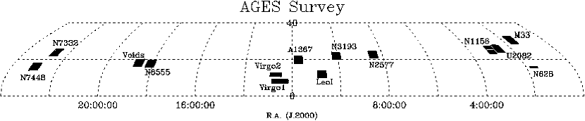
Figure 1: A northern sky map showing the location of the AGES fields.

2.2.1 The Virgo cluster

We have selected two regions of the Virgo cluster to make a comparison of the H i properties of cluster galaxies with those in the field. Both regions avoid the inner 1^∘ of the cluster as the large continuum source associated with M87 limits the dynamic range in the area of about 1 degree around it. Also previous observations indicate very little H i within the cluster core (Davies et al. 2004).

The first region is 10^∘$\times$2^∘ centred on ($\alpha,\delta$) = 12^h 30^m 00^s, 8^∘ 00′ 00″. This region will be imaged as part of the UKIDSS large area survey (Lawrence et al. in prep.) in $J,H$ and $K$ bands. We also have deep $B$-band images of the region taken with the Isaac Newton Telescope, on La Palma. To complement these data, this region will also be observed by GALEX (Martin et al. 2005) in the near (2300 Å) and far ultraviolet (1500 Å) later in 2006. NIR bands are less susceptible to extinction and are thus more accurate measures of stellar mass. Optical-NIR colours can also be used for studying galaxy metallicity and star formation histories. UV is a tracer of ongoing star formation and will allow us to compare current star formation rates with integrated star formation histories. The UV is also useful for searching for signs of star formation in tidal features.

The second region is a 5^∘$\times$1^∘ E–W strip centred on ($\alpha,\delta$) = 12^h 48^m 00^s, 11^∘ 36′ 00″. This strip extends radially towards the cluster edge and will be used to observe changes in galaxy properties with radius from the cluster centre, expanding on the work of Sabatini et al. (2003). This strip extends through the galaxy grouping known as sub-cluster A that is associated with M87 (Binggeli et al. 1993). The results of these observations will be useful for comparing with models of how the cluster environment affects galaxy evolution (tidal stripping, ram pressure stripping etc.).

We will also search for low mass galaxy companions or cluster dwarf galaxies as well as previously unidentified H i clouds. Another interesting study will be to see how baryonic material (stars, X-ray gas, neutral gas) in the cluster is distributed and compare this with the environment surrounding field galaxies.

2.2.2 The local void

We have selected a 5^∘$\times$4^∘ region centred on ($\alpha,\delta$) = 18^h 38^m 00^s, 18^∘ 00′ 00″. We will search for H i signatures that might be associated with very low surface brightness galaxies or with H i clouds devoid of stars. The properties of galaxies detected will provide an interesting comparison with those in more dense environments.

2.2.3 M33 and the Perseus-Pisces filament

This will comprise a 5^∘$\times$4^∘ region centred on ($\alpha,\delta$) = 01^h 34^m 00^s, 30^∘ 40′ 00″. The aim is to map in detail the environment of M33 to search for tidal bridges, HVCs etc. that are signatures of diffuse hydrogen in the Local Group. Westmeier et al. (2005) and Braun & Thilker (2005) have already observed numerous HVCs around M31 and M33, as well as a H i bridge connecting M31 and M33.

M33 will occupy about 1 sq. deg. at the centre of the field. At the distance of M33, the ALFA beam width (3.4′) will be about 0.6 kpc, providing us with superb spatial resolution. The H i mass sensitivity will be as low 2$\times 10^{4}$M_⊙. The Perseus-Pisces filament will become visible behind M33 at approximately 4000–6000 km s^-1.

2.2.4 The cluster A1367

A1367 is a spiral-rich, dynamically young cluster at a velocity of around 6500 km s^-1, and is currently forming at the intersection of two large scale filaments (Cortese et al. 2004). Recent optical and X-ray observations (i.e. Gavazzi et al.2001; Sun & Murray, 2002) suggest that ram pressure stripping and tidal interactions are strongly affecting the evolution of cluster galaxies, making this cluster the ideal place to study the environmental effects on the gas content. The whole cluster will just about fill a 5^∘$\times$4^∘ region centred on ($\alpha,\delta$) = 11^h 44^m 00^s, 19^∘ 50′ 00″. Given the morphology of the cluster we expect many detections including new objects that are more prominent in H i than other wavelengths. The H i mass detection limit at this distance will be approximately 2$\times 10^{8}$ M_⊙.

2.2.5 The Leo I group

This group lies at about 1000 km s^-1 and we will survey a 5^∘$\times$4^∘ region centred on ($\alpha,\delta$) = 10^h 45^m 00^s, 11^∘ 48′ 00″. The group is of particular interest because of the relatively large number of early-type galaxies (e.g. NGC 3377 & NGC 3379) and will make a good comparison with spiral rich groups. We should reach a lower H i mass limit of $\sim 2\times 10^{6}$ M_⊙ at its distance of 10 Mpc.

2.2.6 The NGC 7448 group

NGC 7448 is a Sbc spiral galaxy at a velocity of $\sim$ 2200 km s^-1, with a number of late and early type companions. The group will serve as a good contrast to the Leo I group. We will study a 5^∘$\times$4^∘ area centred on ($\alpha,\delta$) = 23^h 00^m 00^s, 15^∘ 59′ 00″. At the distance of this group (30.6 Mpc) we should reach a H i mass limit of 1.8$\times 10^{6}$ M_⊙.

2.2.7 The NGC 3193 group

NGC 3193, in contrast to NGC 7448, is an elliptical galaxy and there are another 9 known group members all part of a well defined galaxy filament. NGC 3193 has a velocity of 1362 km s^-1 and we will be surveying an area of 5^∘$\times$4^∘ centred on ($\alpha,\delta$) = 10^h 03^m 00^s, 21^∘ 53′ 00″. The lower H i mass limit at this distance (18.9 Mpc) will be approximately 7.0$\times 10^{6}$ M_⊙.

2.2.8 Individual galaxies

This will consist of observations of pairs of galaxies (principle galaxy either early or late type) and very isolated galaxies such as NGC 1156 and UGC 2082. NGC 1156 has no neighbouring galaxies within 10^∘ (Karachentsev, 1996), UGC 2082 has no neighbour within 5 ^∘ in the Nearby Galaxies Atlas (Tully & Fisher, 1987). Details are shown in Table 1.

2.2.9 AGESVOLUME

In addition to the data collected from the targets mentioned above, the large system bandwidth (100 MHz) will allow us to simultaneously sample a much deeper volume of the universe and search for more distant galaxies along the line of sight out to $cz\sim 19000$ km s^-1. The detection limit at this distance will be M${}_{HI}=1.4\times 10^{9}$M_⊙. This is the AGESVOLUME and will be a very important part of the project, providing information on the HIMF, the baryonic mass density of neutral gas and the distribution of H i.

Table 1: H i Survey fields for individual galaxies.

Galaxy	RA	dec.	Type	$V_{sys}$	Distance	H i mass limit	Comments	Survey
	($h~{}m~{}s$)	(∘ ′ ″)		(km s-1)	(Mpc)	(M⊙)		area
NGC 6555	18 06 00	17 30 00	Sc,	2225	30.9	1.9$\times 10^{7}$	paired with	5∘$\times$4∘
			face-on				NGC 6548
NGC 2577	08 24 00	22 30 00	S0	2057	28.6	1.6$\times 10^{7}$	paired with	5∘$\times$4∘
							UGC 4375
NGC 7332	22 36 00	23 48 00	S0 (pec)	375	5.2	5$\times 10^{5}$	paired with	2.5∘$\times$2∘
							NGC 7339
UGC2082	02 36 00	25 48 00	Sc,	696	9.7	1.8$\times 10^{6}$	very	2.5∘$\times$2∘
			edge-on				isolated
NGC 1156	03 00 00	25 12 00	Irr	375	5.2	5$\times 10^{5}$	very	2.5∘$\times$2∘
							isolated

2.3 Observing strategy

A number of observing strategies were considered for the survey, which involved pointed observations, drift scanning, driven scanning techniques or combinations thereof. The successful observing method had to strike the right balance between data quality and observing efficiency.

Giovanelli et al. (2005) describe in detail an observing mode known as drift scanning. As the name suggests, the array is kept at a fixed azimuth and elevation while the sky drifts overhead. The benefits of this technique are that the telescope gain remains constant and the system temperature only varies slowly over a single scan. Standing waves set up between the receiver and the dish cause ripples to appear in the spectrum baseline. These waves are quasi-periodic and depend on the polarisation, the geometry of the dish and the location of continuum sources in the main beam and sidelobes. Hence each beam and polarisation will have a different baseline ripple at any given time. This baseline ripple can cause confusion with low signal sources so limiting its effect is highly desirable. The drift scan technique has the advantage that this ripple is more or less constant over the course of the scan. It is then possible to accurately estimate the ripple and remove it from the data during the data reduction. The benefits made the drift scan highly desirable for our own observations.

The Earth’s rotation rate governs the on source time in a drift scan. For Arecibo this means that each point in the sky takes 12s to cross the beam at 1.4 GHz. 25 separate scans are then required per point to reach the 300s integration time. Since the technique used in ALFALFA only allows for scans taken along the meridian (Giovanelli et al. 2005) it was necessary to adapt the method to allow us to conduct scans before and after transit, and hence build up sky coverage more quickly.

In order to compensate for the change in parallactic angle, and thus achieve uniform sky coverage, ALFA must be rotated before every scan. The geometry of the Gregorian system projects a slightly elliptical beam pattern on the sky. The projected beams are also slightly elliptical (see Fig. 2). As a result of these effects, once the array is rotated to produce equidistant beam tracks, the beam separation is slightly larger than that required for Nyquist sampling. To attain fully sampled sky coverage it is necessary to stagger the declination of individual scans by $\sim$1′ (half the beam separation). An IDL routine has been developed to calculate the rotation angle and the starting coordinates and LSTs in advance of every observing run. This staggering is arranged such that every beam covers the same patch of sky helping to combat variations in gain between the beams. Another benefit of this method is to reduce the impact of sidelobe contamination. This effect is discussed separately in the next section.

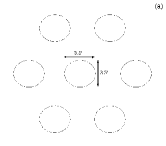
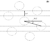
Figure 2: An illustration of the projected ALFA footprint, (a) unrotated with respect to the direction of the scan, and (b) rotated to produce equidistant beams of 2.1′ separation. Dotted lines indicate the individual beam tracks across the sky.

2.4 Data reduction

Data reduction will be performed using the aips++ packages livedata and gridzilla (Barnes et al. 2001), developed by the Australian Telescope National Facility (ATNF). These packages were originally designed for the HIPASS and HIJASS surveys but were modified to accept the Arecibo CIMAFITS file format. livedata performs bandpass estimation and removal, Doppler tracking and calibrates the residual spectrum. It also has the ability to apply spectral smoothing if required. Bandpass calibration can be performed using a variety of algorithms, all based around the median statistic. The median has the advantage that it is more robust to outliers than the mean statistic. This property makes the median estimated bandpass more resistant to radio frequency interference (RFI).

gridzilla is a gridding package that co-adds all the spectra using a suitable algorithm, to produce 3-D datacubes. The user has full control over which beams and polarisations to select, the frequency range, the image size and geometry, pixel size and data validation parameters as well as the gridding parameters themselves. Various weighting functions are available for gridding the data. The output datacube has two spatial dimensions and the spectral dimension can be chosen by the user to be frequency, wavelength or velocity (numerous conventions are available for each choice). Full details of the bandpass estimation and gridding technique are given in Barnes et al. (2001).

The sidelobes for the central beam are symmetric, while sidelobe levels for each of the outer beams are highly asymmetric, as shown in Fig. 3. Our ability to regain low column density emission could be highly compromised if they are not corrected, particularly near bright objects or very extended objects. In the final, gridded data, each beam has contributed equally to each pixel apart from at the extreme edges of the map where sky coverage is not complete. Fig. 3 highlights the radial alignment of the peaks of each of the sidelobes. When median gridding is applied this means that in order for a pixel to be significantly contaminated by sidelobe emission, the source must appear in more than three of the beams. Point sources can therefore be considered free of sidelobe contamination. It should be noted that there is likely to be some low level contamination in extended objects and we are investigating ways to reduce this.

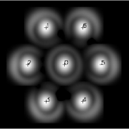
Figure 3: An illustration of the ALFA beam footprint to emphasise the strength and symmetry of the sidelobes. (a) A highly stretched image of the combined response of all seven ALFA beams, the image size is 32′$\times$32′. (b) The beam separations have been stretched to 2.5 times the true separations to highlight the sidelobes of the beams. The angular scales of each beam is correct and unchanged. The image size in this case is 48′$\times$48′. (Figures appear courtesy of Carl Heiles.)

3 Precursor observations

The observations were taken using the 305m radio telescope located at Arecibo, Puerto Rico. We were allocated a total of 86 hours which was split between different observing strategies, as part of a ‘shared risk’ strategy. The drift scan observations received 42.5 hours and we discuss only these observations in this paper. The observations were taken over 22 nights between November 19th 2004 and December 18th 2004. No radar blanking was used because it was not functional at the time, leading to several sources of RFI as discussed later. System malfunctions were inevitable during a testing run such as this, but only four nights’ of observing were affected. This corresponded to approximately 10 hours lost time.

3.1 The NGC 628 group

The group is centred round a large, face-on spiral, NGC 628 and the peculiar spiral NGC 660. NGC 628 is associated with several companions: UGC 1104, UGC 1171, UGC 1176(DDO13), UGC A20 and KDG10. NGC 660 also has a couple of companions: UGC 1195 and UGC 1200 (Fig. 4). Most of the companions are star forming dwarf irregulars and together these galaxies form a gas-rich group analogous to the Local Group (Sharina et al., 1996). The recessional velocity of NGC 628 is $\sim$660 km s^-1 (Huchra, Vogeley & Geller, 1999; de Vaucouleurs, 1991; Kamphuis & Briggs, 1992) placing it at approximately 10 Mpc away (assuming no peculiar motion and $H_{o}$ = 75 km s^-1 Mpc^-1, as used in Briggs, 1986). Supernovae measurements (Hendry et al. 2005) give a distance measurement of 9.3$\pm$1.8 Mpc.

NGC 628 has a very narrow velocity width, $W_{50}=56$ km s^-1 (Kamphuis & Briggs 1992). It is close enough to allow detection of low-mass H i objects with only M${}_{HI}=2\times 10^{6}$M_⊙ of neutral hydrogen, but separated enough from local Galactic gas to be able to detect any high velocity gas associated with the galaxy. Kamphuis & Briggs (1992) looked at this galaxy at 21cm with the VLA and discovered high velocity gas on the outskirts of NGC 628 but nothing that could be considered HVCs. A few years earlier another survey (Briggs, 1986) revealed a new, low-mass companion, dw0137+1541 (M${}_{HI}=7\times 10^{6}$M_⊙). This group has also been covered by the HIPASS northern extension. The interesting aspects of the group and the availability of comparison observations from other instruments made it a natural choice for precursor observations using a new instrument.

3.2 Observations and data reduction

A 5^∘$\times$1^∘ field was chosen centred on a position halfway between NGC 628 and the nearest dwarf UGC 1176 (Fig. 4). The region includes NGC 628, UGC 1176, UGC 1171, KDG010 and dw0137+1541. The observing band was centred on 1381 MHz, giving a heliocentric velocity range of $-$2270 km s^-1 to $+$20079 km s^-1. The roll off at the edge of the bandpass due to the filter reduces the sensitivity for about 1000 km s^-1 at either end.

Figure 4: The NGC 628 group with the observed field outlined. Group members are denoted by a cross, dw0137+1541 has not been included due to its proximity to UGC 1176 and UGC 1171.

The strategy consisted of two sets of scans. The first set covered the entire field on one night while the second set were offset by half a beam width as shown in Fig. 5. This observing strategy differs slightly from those described in section 2.3 since in this technique individual points in the sky are only covered by one or two beams. This was a necessary sacrifice since the tools that assisted in the design of the survey strategy were still in development.

Figure 5: An illustration of how the sky coverage is built up over two nights of observations. The declination axis has been stretched for convenience. The solid lines represent the central beam tracks, the dashed lines mark the outer beam tracks. On the first night (a), 5 separate drift scans are performed to cover the 5^∘$\times$1^∘ area. On the second night (b), exactly the same pattern is reproduced offset by half the beam separation (the outer beams from the second night at denoted by dotted lines). On subsequent nights the two patterns are alternated to build up integration time and also maintain uniform sky coverage. Due to observation scheduling it was often necessary to drop the northern-most scan. Galaxies are marked with a cross, with NGC 628 marked for guidance. Refer to Fig. 4 to locate other group members.

Observations were planned such that the central drift scan was always conducted close to the meridian. Due to the time limits imposed by the telescope schedule, this often meant only four of the five scans were completed. With the available time we were able to cover most of the region to a uniform depth using 16 nights’ data. Due to observing constraints, the region north of 16^∘ 06′ 00″ was often omitted from the observing run, and hence this region was only observed successfully on 6 nights. This is illustrated by Fig. 6, which shows the number of spectra that were obtained for each pixel in the final, gridded data. This was reflected in the noise quality of the final data which was significantly poorer for the more sparsely covered region (above $\sim$16^∘06′00″). Calibration was performed at the beginning of every scan using a high-temperature noise diode that was injected into the beam for a duration of 1s. We integrated every 1s for each of the 7 beams, both polarisations and 4096 channels as 4-bit floating point numbers. Over a 20 minute drift scan this equates to a total file size of $\sim$ 395 Mb.

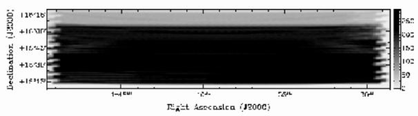
Figure 6: A map showing the sky coverage in the final data. The number of spectra that contributed to each pixel is shown as a greyscale from least (light), to most (dark). The region above 16^∘ 06′ 00″ was less well covered than the remaining region due to observing time constraints.

After data reduction, the resulting fits datacube from gridzilla has dimensions of RA, dec and velocity/frequency. The 5^∘$\times$1^∘ region was gridded using a median gridding technique into 1′$\times$1′ pixels, each of which contains a 4096 channel spectrum. This produced a $\sim$365 Mb file. Initial investigations of the effects of RFI and the behaviour of noise in the data were conducted using idl. Detailed analysis of the NGC 628 group was performed using miriad, gipsy and karma.

3.3 Radio Frequency Interference (RFI)

Man-made RFI is now, unfortunately, a constant source of contamination at most radio observatories. At Arecibo in the L-band there are a number of RFI sources. The L3 GPS satellite appears at approximately 1381 MHz. There are also several narrow contributions from aircraft radar at FAA and Punta Salinas in the range 1200–1381 MHz. While RFI from Punta Salinas was not noticed during the observations, two sources were noticed at 1350 MHz (FAA radar) and 1381 MHz (L3 GPS). These interference sources were present throughout the observing runs but other sources were only noticed occasionally. The median filtering applied by livedata and gridzilla is very robust to intermittent sources of RFI but can do nothing for constant sources. As a result several channels were contaminated around 1351 MHz and 1381 MHz. These channels were included in the final data, to allow for the possibility of detecting bright sources that might still be visible.

In addition to these sources of RFI there was also a varying source. While the RFI was quite narrow, usually occupying a few channels, it would shift frequencies in a quasi-periodic fashion contaminating up to 60 MHz of the band. There was also a harmonic that would drift in an out of our bandwidth. Figs. 7 & 7 are two graphs showing the noise in each channel of the spectrometer, for two identical regions of sky taken over two consecutive nights. The first night’s data are contaminated by this transient RFI source, the second night’s data are free of it. The effect on the quality of the final data is significant, causing a rise in the noise level throughout the band. The RFI source has been attributed to equipment in the focus cabin and has now been eliminated.

Figure 7: The impact of the persistent, frequency-varying RFI on the data quality. Each figure shows the rms noise per channel from observations on consecutive nights (a) with the interference present and (b) without the interference. Both datasets represents averages taken over the same source-free patch of sky.

3.4 Noise behaviour

By combining multiple observations of the survey field it is possible to build up the effective integration time and hence increase the depth of the survey. One would expect that as more observations are taken, the noise level in the combined data should fall. Datacubes were produced for 1, 2, 4, 8, and 16 nights’ observations. Since the integration time each night was the same (12s beam^-1), this was equivalent to 12, 24, 48, 96, and 192s beam^-1. A robust mean noise value was then calculated for each datacube, using the idl astro library routine resistant_mean within a large region of sky that didn’t contain sources over the inner 3696 channels. The data were fitted using a least-squares fit. In theory we would expect the noise level to be, $\sigma$ $\propto t^{-0.5}$ where $t$ is the integration time. Fig. 8 shows how the rms noise level varies with the integration time. The line fit indicates the noise decreases as $t^{-0.49\pm 0.06}$ which is in very good agreement with the $t^{-0.5}$ dependence as predicted. This represents 16 nights’ data which provided uniform coverage for most of the region. Following this predicted trend, a final noise level of 0.95 mJy for a velocity resolution of 10.3 km s^-1 could have been achieved if all 25 nights’ observing (300s beam^-1) had been successful.

Figure 8: The effect of co-adding successive nights observations results in the expected reduction in the rms noise value, i.e. $\sigma\propto t^{-0.5}$.

To investigate the Gaussianity of the noise in the final co-added data (t${}_{int}=192s$), a source-free region of sky was chosen and the noise in each channel for each pixel was recorded. The values were binned into 100 equally spaced bins. The noise distribution about the mean value was then compared to a Gaussian distribution. The values lay very close to a Gaussian, distributed about zero (Fig. 9). From Fig. 9 there is a slight excess in noise at $\sim$3.0 mJy ($\sim 3\sigma$). This is probably due to numerous sources lying just below the detection limit.

Figure 9: (a) The distribution of flux values within an apparently blank patch of sky in the reduced datacube is well fit by a Gaussian distribution, centred on -0.1 mJy. The data points are represented by crosses and the solid line is the Gaussian fit (b) There is a departure from Gaussianity between 2.5–4.0 mJy corresponding to 2.3–3.6$\sigma$. This is possibly due to very low-level sources within the region that were not detected by eye.

3.5 Baseline stability

The quality of the final data is highly dependent on the stability of our baselines. It is extremely important therefore to examine the baseline before any fitting is applied to it, and confirm that the drift-scanning technique is producing the stable baselines expected. Observations were chosen from a night in which there was no contamination by the persistent, variable RFI. Comparisons were then made from spectra taken at the beginning of a scan to those at the end of the scan.

Fig. 10 shows, for each individual beam and polarisation, the percentage difference between the first 100 spectra and the last 100 spectra within one scan. The baseline remains stable to within 0.1% over the duration of a scan.

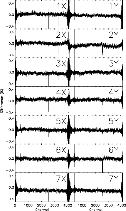
Figure 10: Percentage variation of the raw bandpass over a single scan for each individual beam and polarisation. Each raw bandpass remains unvarying to within $\sim$0.1%.

4 Results

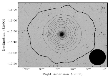
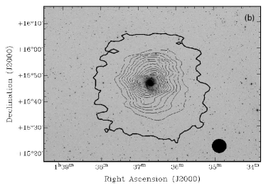
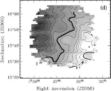
Figure 11: NGC 628 (a) HIPASS H i contours overlaid on a POSS II image. Contours ($\times 10^{18}$ cm^-2): 2.8 (3$\sigma$), 50, 100, 150, 200, 250, 300, 350, 400, 450, 500. The solid circle illustrates the size of the HIPASS beam. (b) AGES H i contours overlaid on a POSS II image. Contours ($\times 10^{18}$ cm^-2): 2.2 (3$\sigma$), 100, 200, 300, 400, 500, 600, 700, 800, 900, 1000, 1100. The solid circle illustrates the size of the AGES beam.(c) H i velocity profiles: HIPASS is shown as the dashed line, AGES as the solid line. (d) Velocity field from AGES data. Isovelocity contours increase from light to dark: 635, 640, 645, 650, 655, 659, 660, 665, 670, 675, 680, 685, 690 km s^-1.

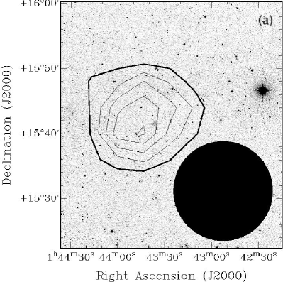
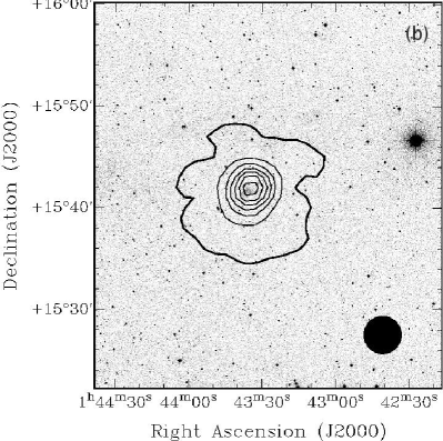
Figure 12: KDG 010 (a) HIPASS H i contours overlaid on a POSS II image. Contour values: 1, 2 (3$\sigma$), 3, 4, 5 ($\times 10^{18}$cm^-2). The solid circle illustrates the size of the HIPASS beam. (b) AGES H i contours overlaid on a POSS II image. Contour values: 2 (3$\sigma$), 20, 40, 60, 80 ($\times 10^{18}$cm^-2). The solid circle illustrates the size of the AGES beam. (c) H i velocity profiles: HIPASS is shown as the dashed line, AGES as the solid line.

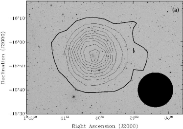
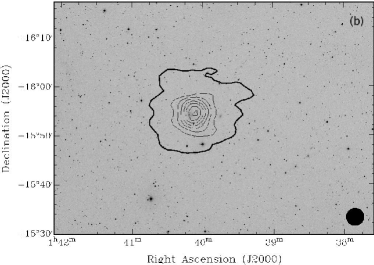
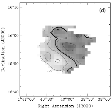
Figure 13: UGC 1176 (a) HIPASS H i contours overlaid on a POSS II image. Contours ($\times 10^{18}$ cm^-2): 2 (3$\sigma$) 5, 10, 15, 20, 25, 30, 35, 40, 45. The solid circle illustrates the size of the HIPASS beam. (b) AGES H i contours overlaid on a POSS II image. Contours ($\times 10^{18}$ cm^-2): 2 (3$\sigma$), 60, 120, 180, 240, 300, 360, 420. The solid circle illustrates the size of the AGES beam. (c) H i velocity profiles: HIPASS is shown as the dashed line, AGES as the solid line. (d) Velocity field from AGES data. Isovelocity contours increase from light to dark: 620, 625, 630, 634, 635, 640.

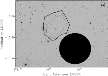
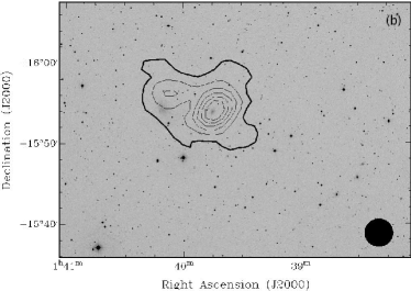
Figure 14: UGC 1171 & dw0137+1541 (a) HIPASS H i contours overlaid on a POSS II image. Contours ($\times 10^{18}$ cm^-2): 2 (3$\sigma$), 3. The solid circle illustrates the size of the HIPASS beam. (b) AGES H i contours overlaid on a POSS II image. Contours ($\times 10^{18}$ cm^-2): 2 (3$\sigma$), 5, 10, 20, 30. The solid circle illustrates the size of the AGES beam. (c) H i velocity profiles for UGC 1171 and dw0137+1541: HIPASS data for UGC 1171 is shown as the dashed line, AGES data for UGC 1171 is the solid line. Dw0137+1541 is shown by the dash-dot line.

The reduced datacube was masked to isolate all the H i emission from each member of the NGC 628 group and then moment maps were constructed for each galaxy. Moment 0 maps were constructed to illustrate the H i distribution over the channel range occupied by each galaxy. Where the galaxy was resolved, moment 1 maps (velocity fields) were also produced. These moment maps are shown in Figs. 11–14 and also include the velocity profile of each galaxy. For comparison purposes we also provide moment 0 maps produced from HIPASS data. None of the galaxies were resolved by HIPASS and so there are no velocity fields from HIPASS data.

The 3$\sigma$ column density limit is around 2$\times 10^{18}$ cm^-2 in the integrated H i maps for both HIPASS and the AGES precursor. The benefit of our increased spectral resolution is immediately clear in the velocity profiles. The improvement in spatial resolution is also highlighted by the detection of dw0137+1541. This dwarf is so close to UGC 1171 that it is undetected in the HIPASS data but is clearly visible in the AGES data (Fig. 14b) at position $(\alpha,\delta)=01h\/40m\/03s$, +15^∘ 56′ 00″. Fig. 14(b) suggests that UGC 1171 & dw0137+1541 are embedded in a neutral gas envelope extending from northeast to southwest. This could be an effect of beam smearing since there is no hint of extended emission in Briggs et al. (1986), but it is possible that it is real and has been resolved out by the synthesised beam of the VLA.

An important step is to compare the velocity profiles from AGES and HIPASS to see if the flux calibration is being performed correctly. From Figs. 11–14 the fluxes calculated from the AGES data are generally in agreement with the HIPASS data. The most probable reason for discrepancies is that the gridding technique responds differently to sources of different size and strength. The problem is that the gridding technique tends to overestimate the flux of extended objects (objects comparable to or larger than the beam size). This was an expected side effect of the gridding process and Barnes et al. (2001) simulated observations in the HIPASS data using sources of known flux and size to quantify the effect and calculate correction values. Another side effect of the technique is to produce larger gridded beam sizes for stronger sources (see Tables 2 & 3 in Barnes et al. 2001).

We have corrected for this as follows. First the ratio of the AGES source size to the AGES beam was found. The source size was measured from higher resolution H i data (Briggs, 1986; Briggs, 1992). This ratio was multiplied by the HIPASS mean observing beam size (14.4′) to find the size of a hypothetical HIPASS source that would produce the equivalent source/beam ratio. Table 3 in Barnes et al. (2001) was then used to find the HIPASS flux-weighted beam area for this hypothetical source. The ratio of the HIPASS flux-weighted beam area to the mean observing beam area was then calculated. Finally the AGES observing beam area was then multiplied by this ratio to get the AGES flux-weighted beam area. The integrated flux was then simply the summed AGES flux from the source multiplied by the AGES pixel size divided by the AGES flux-weighted beam area.

There are other possible sources of inaccuracy in the AGES data. The gain calibration did not take into account the telescope’s response at different zenith angles - beyond a zenith angle of $\sim$15^∘ the Arecibo 305m dish is known to lose sensitivity since only part of the dish is illuminated. This effect was limited since very few scans were taken at zenith angles greater than 15^∘.The system temperature is also known to vary over the frequency range of the system which was not taken into account during the data reduction. Steps are underway to document these variations so that they may be included in future revisions of livedata and gridzilla.

Table 2 shows the measured parameters from AGES, for each galaxy, compared to those measured from HIPASS and also from other previous surveys (Kamphuis & Briggs, 1982; Briggs, 1986; Huchtmeier, 2003). Positions were found from applying the fitting routine imfit within miriad to the flux map integrated over the galaxy’s velocity extent. Uncertainties are shown in brackets after each measurement. Positional uncertainties for AGES data were estimated from fitting NRAO VLA Sky Survey (Condon et al., 1998) sources to a continuum map produced from our data. For AGES, positions of NVSS sources were found to be accurate to within $\pm$30″. Uncertainties in position from the HIPASS data were taken from Zwaan et al. (2003). The AGES positions agree with HIPASS and previous measurements to within the measured uncertainties.

The uncertainties in each of the H i properties depend on the S/N of the source, the velocity width of the source, the velocity resolution and the shape of the spectrum. An excellent summary of techniques for estimating the uncertainties in these H i properties is given in Koribalski et al. (2004) and references therein. The uncertainty in the integrated flux density is given by

$$\sigma(F_{HI})=4\times SN^{-1}(S_{peak}F_{HI}\delta v)^{1/2}$$ (1)

where $S_{peak}$ is the peak flux, SN is the ratio of $S_{peak}$ to $\sigma(S_{peak})$, F_HI is the integrated flux and $\delta v$ is the velocity resolution of the data. $\sigma(S_{peak})$ is found to increase in extended sources, regions of high 20-cm continuum emission and it also increases with rising flux density values. We adopt the estimate of Koribalski et al. (2004) that ($\sigma S_{peak})^{2}$ = rms² + (0.05 $S_{peak})^{2}$.

The uncertainty in the systemic velocity is given by:

$$\sigma(V_{sys})=3\times SN^{-1}(P\delta v)^{1/2}$$ (2)

where $P=0.5\times(W_{20}-W_{50})$, which is simply a measure of the steepness of the profile edges. Errors in the widths are given by $\sigma(W_{50})=2\times\sigma(V_{sys})$ and $\sigma(W_{20})=3\times\sigma(V_{sys})$. Distances are based on pure Hubble flow and the associated errors arise from the errors in the integrated flux.

Table 2: H i measurements of the NGC 628 group.

Survey	RA	DEC	Vsys	W50	W20	FHI	MHI
	(2000)	(2000)	(km s-1)	(km s-1)	(km s-1)	(Jy km s-1)	($\times 10^{8}$M⊙)
NGC 628
AGES	1 36 41.9 (2.0)	15 47 44 (30)	659.2 (1)	56 (2)	73 (3)	352.6 (3.7)	9.1 (0.1)
HIPASS	1 36 42.0 (4.5)	15 47 34 (48)	654 (3)	50 (6)	75 (9)	431 (13)	11.0 (0.3)
Kamphuis	1 36 42.0 (1.0)	15 47 12 (14)	657 (0.7)	56 (1)	—	470.1	12
& Briggs (1982)
KDG010
AGES	1 43 34.9 (2.0)	15 41 48 (30)	792 (1)	34 (2)	49 (3)	3.13 (0.28)	0.80 (0.07)
HIPASS	1 43 46.5 (4.6)	15 42 48 (48)	787 (5)	27 (10)	45 (15)	2.0 (1.1)	0.5 (0.3)
Huchtmeier	1 43 37.2 (4.6)	15 41 43 (48)	788.9 (0.4)	32 (1.1)	—	2.35	0.6
(2003)
UGC 1176
AGES	1 40 06.0 (2.0)	15 54 45 (30)	634 (1)	36 (2)	54 (3)	27.4 (1.9)	7.0 (0.5)
HIPASS	1 40 08.4 (4.6)	15 55 06 (48)	628 (2)	40 (4)	58 (6)	28.2 (4.3)	7.2 (1.8)
Briggs (1986)	1 40 07.7 (1.0)	15 53 55 (14)	629 (1)	38 (1)	—	30.17	7.7
UGC 1171
AGES	1 39 38.6 (2.0)	15 55 19 (30)	743 (1)	29 (2)	41 (3)	1.46 (0.14)	0.37 (0.04)
HIPASS	1 40 00.2 (4.6)	15 53 56 (48)	743 (2)	27 (4)	45 (6)	2.2 (1.2)	0.56 (0.3)
Briggs (1986)	1 39 44.2 (1.0)	15 54 01 (14)	740 (3)	23 (4)	—	1.80	0.5
dw0137+1541
AGES	1 40 03.9 (2.0)	15 55 45 (30)	749 (1)	28 (2)	47 (3)	0.39 (0.21)	0.10 (0.05)
HIPASS	—	—	—	—	—	—	—
Briggs (1986)	1 40 09.2 (1.0)	15 56 16 (14)	750 (5)	23 (10)	—	0.27	0.07

One of the aspects of AGES is the potential to detect diffuse H i that is located in the intergroup or intracluster medium. The high resolution of the AGES observations, however, has the advantage of allowing differentiation between H i that may be associated with a hitherto unknown LSB galaxy in the group (for instance, see Pisano et al. 2004) and a more extended, smooth, diffuse component or extended clump of emission within the overall structure of the group. The nature of the distribution of baryonic material in this medium (e.g. White et al. 2003) can provide interesting constraints on structure formation (see Mihos et al. 2005; Osmond et al. 2004). In Fig. 4, the rectangular survey area has physical dimensions of approximately 1 Mpc$\times$200 kpc. This provides an indication of how spread out this group is. The overall physical radius of the NGC 628 extended group is approximately 1.5 Mpc with a relatively low velocity dispersion of 100–150 km s^-1 depending on which choices are made for group membership. Overall its physical extent is similar to our Local Group, but it contains more than just 3 bright galaxies (all the listed UGC and NGC galaxies are more massive than M33).

There appears to be no evidence of intra-group gas down to a H i column density of 2$\times 10^{18}$ cm^-2 integrated over a velocity width, $\Delta v$ = 50 km s^-1. In Table 2, the sum of the detected H i masses is approximately 2$\times 10^{10}$M_⊙, of which 1/2 belongs to NGC 628 and its extended H i emission. Excising that region from the search area and using our observed upper limit on column density of any H i emission, leads to an upper limit of 5$\times 10^{8}$M_⊙ for the integrated smooth, intergroup H i mass that might be distributed between NGC 628 and KDG 010. This is less than 3% of the H i mass observed to exist in the bodies of the galaxies and strongly suggests that tidal interactions in this gas-rich group of galaxies have not been very robust in removing H i from the host galaxies. This result is consistent with the symmetry and pronounced lack of tidal distortion of the extended H i emission around NGC 628. Perhaps this suggests that loose galaxy structures, like the NGC 628 group and the Local Group are too dynamically young for sufficient interactions to have occurred.

4.1 Objects beyond the NGC 628 group

Due to the large observing bandwidth offered by the WAPPs (100 MHz) it was expected that a number of background objects would also be detected. The datacube was examined by eye for more distant objects and 22 other objects were detected out to a velocity of $cz$=17500 km s^-1. Including the NGC 628 group this gives a detection rate of 5.4 objects deg^-2. This implies that the total number of galaxies detected by AGES will be $\sim$1500. The ALFALFA survey (Giovanelli et al. 2005) has predicted that they will detect a 20000 objects over an area of 7000 deg², giving an average detection rate of 2.9 deg^-2.

Another important aspect of this project is to identify potential optical counterparts. Positional data is not enough for optical associations, it is also necessary to obtain optical spectral data to compare the redshift of the gas with that of the visible galaxies in the image field. If the positional or spectral data of the radio observations don’t correlate with that of the optical observations, then an optical object cannot be considered the optical counterpart to the H i emission.

NED was used to search for objects within a 3′ radius of each H i detection. 6′$\times$6′ POSS II images, taken from the SuperCOSMOS database, were also examined for possible optical counterparts. Of the 22 detections, 9 appear to be previously uncatalogued and none of the objects are listed in NED as having previous H i measurements. SDSS redshift data is available for only 3 objects, but these compare favourably with the H i redshifts as described below. The H i detections are listed in Table 3 along with any objects listed in NED within a 3′ radius. The final column in Table 3 shows the angular distance between the centre of the H i detection and the NED object’s position. Fig. 15 shows the SuperCOSMOS images for each object, centred on the H i detection, together with the H i spectra. The Arecibo beam is represented by the circle and is to scale. Optical detections within the Arecibo beam have been identified with an arrow and previously catalogued objects have been labelled. Descriptions of the images and the corresponding spectra are given below. Although some objects coincide with the centre of the H i emission, one should bear in mind that without optical redshift data, it is impossible to say for certain whether or not these objects are associated with the gas.

	RA	DEC	Vsys	Distance	W50	W20	FHI	MHI	Previously catalogued	Angular	M${}_{HI}/$LH
AGES ID	(2000)	(2000)	(km s-1)	(Mpc)	(km s-1)	(km s-1)	(Jy km s-1)	($\times 10^{8}$M⊙)	objects	separation
										(arcmin)	M${}_{\odot}/$L⊙
J013149+152353	01 31 48.9	15 23 53	10705 (3)	146	178 (6)	220 (9)	1.44 (0.11)	72.2	SDSS J01314980+1523265	0.5	0.9
J013204+152947	01 32 04.1	15 29 47	13196 (7)	178	326 (14)	400 (21)	1.01 (0.11)	75.5	SDSS J013204.6+153001.2	0.3	0.1
									2MASX J01320599+1529298	0.5	0.5
J013313+160139	01 33 12.9	16 01 39	8895 (3)	122	138 (6)	194 (9)	1.69 (0.11)	59.0	2MASXi J0133132+160125	0.2	—
J013323+160222	01 33 22.8	16 00 21	8587 (1)	118	69 (2)	81 (3)	0.07 (0.02)	2.1	New	—	—
J013538+154850	01 35 38.0	15 48 50	8012 (3)	110	132 (6)	153 (9)	0.61 (0.08)	17.5	New	—	—
J013718+153635	01 37 18.0	15 36 35	8174 (4)	112	144 (8)	169 (12)	0.46 (0.08)	13.7	NVSS J013714+153722	1.2	0.3
J013807+154328	01 38 07.0	15 43 28	13237 (2)	179	162 (4)	169 (6)	0.60 (0.08)	45.4	New	—	—
J013827+154728	01 38 26.8	15 47 28	8339 (2)	114	182 (3)	201 (5)	1.74 (0.11)	53.4	New	—	—
J013917+154613	01 39 17.1	15 46 13	17080 (5)	228	51 (9)	98 (14)	0.27 (0.05)	33.5	New	—	—
J013953+151955	01 39 52.7	15 19 55	16806 (6)	224	231 (12)	284 (18)	0.43 (0.07)	51.1	SDSS J013955.02+152036.7	0.9	—
J013956+153135	01 39 56.2	15 31 35	17343 (7)	231	105 (14)	214 (21)	0.42 (0.07)	53.7	New	—	—
J014013+153319	01 40 13.0	15 33 19	17052 (7)	227	535 (14)	566 (21)	1.33 (0.13)	163.0	2MASX J01401331+1533345	0.3	0.2
J014025+151903	01 40 25.2	15 19 03	16848 (5)	225	44 (9)	101 (14)	0.31 (0.06)	36.7	2MASX J01402402+1518240	0.7	0.2
J014033+160513	01 40 32.6	16 05 13	13017 (4)	176	101 (8)	152 (12)	0.59 (0.07)	42.6	2MASXi J0140360+160414	1.3	—
J014430+161502	01 44 30.3	16 15 02	5020 (2)	70	107 (3)	121 (5)	0.61 (0.07)	7.0	New	—	—
J014524+155923	01 45 23.7	15 59 23	5050 (4)	70	34 (7)	60 (11)	0.18 (0.04)	2.1	New	—	—
J014630+154332	01 46 30.4	15 43 32	17495 (3)	232	132 (6)	167 (9)	0.73 (0.09)	92.7	2MASX J01463012+1543250	0.1	0.4
J014644+155622	01 46 44.0	15 56 22	7063 (5)	97	27 (10)	51 (15)	0.10 (0.05)	2.2	2MASX J01465179+1557192	2.1	0.07
J014719+155603	01 47 19.1	15 56 03	5191 (3)	72	86(7)	104 (11)	0.35 (0.07)	4.3	NVSS J014722+155737	1.8	—
J014742+161317	01 47 41.7	16 13 17	4890 (3)	68	138 (6)	177 (9)	1.02 (0.09)	11.1	2MASXi J0147459+161318	1.0	—
J014752+155855	01 47 51.7	15 58 55	17514 (11)	233	450 (22)	578 (33)	1.59 (0.13)	200.0	2MASX J01475424+1558247	0.8	1.0
									2MASX J01475424+1559387	1.0	—
J014834+152756	01 48 33.7	15 27 56	12985 (4)	175	114 (8)	129 (12)	0.50 (0.07)	36.3	New	—	—

Table 3: H i properties of objects detected beyond the NGC 628 group.

AGES J013149+152353 This signal coincides with the SDSS galaxy, SDSS J013149.81+152326.5. There is an optical redshift available for this galaxy placing it at $cz=$10717 km s^-1. The radio data place the galaxy at a recessional velocity of $cz=$10705 km s^-1. SDSS J013149.81+152326.5 is a spiral galaxy and this morphology is reflected in the H i profile. This galaxy appears to be somewhat isolated since there are no galaxies reported in this region within 1700 km s^-1.

AGES J013204+152947 The SDSS galaxy, SDSS J013204.6+153001.2, falls almost in the centre of the Arecibo beam. It has an optically measured redshift of $cz=$13195 km s^-1 from the SDSS. Our radio measurement of the recessional velocity is $cz=$13196 km s^-1. The good agreement between the positional and redshift data make it almost certain that this is the source of the H i. This galaxy has a red optical colour ($g-r\sim$0.75 mag) typically observed in early type galaxies (Bernardi et al. 2003). Moreover the SDSS nuclear spectrum shows a red continuum and no sign of recent star formation (i.e. no emission lines). A similar red colour ($g-r\sim$0.84 mag) is associated with the companion, 2MASX J01320599+1529298, which lies within the beam.

AGES J013313+160139 Spiral structure is clearly seen in the H i profile and is probably coming from 2MASXi J0133132+160125 which lies in the centre of the beam.

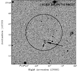
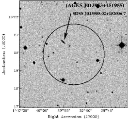
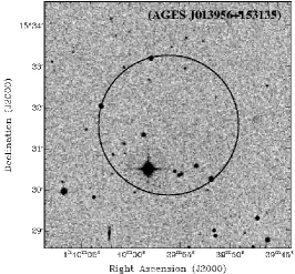
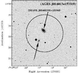
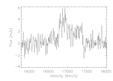
Figure 17: continued

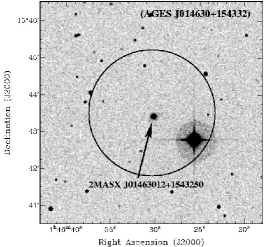
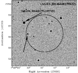
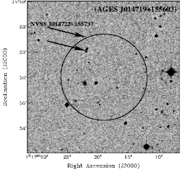
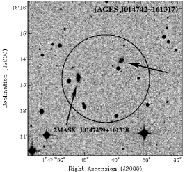
Figure 19: continued

AGES J013323+160222 The H i profile for this object is not the large S/N signal centred at $cz\sim$8650 km s^-1 in Fig. 19, but that located at $cz\sim 8350$ km s^-1. The large signal is coming from AGES J013313+160139 (Fig. 17). AGES J013323+160222 is admittedly a marginal detection ($\sim 3\sigma$) and will no doubt require deeper H i observations to confirm. There is a faint smudge visible in B and R (not shown) located at 01^h 33^m 14.8^s, 16^∘ 02′ 56″.

AGES J013538+154850 The H i position is likely to be coming from the spiral located near the centre of the image. This is supported by the H i profile which is a typical spiral, but only optical redshift data would really tie down the H i emission to this galaxy.

AGES J013718+153635 The H i profile for this object is typical of a spiral galaxy. Tying it down to a single galaxy is difficult though. There is a 21cm continuum source (NVSS J013714+153722) located at a distance of 1.2′. This frame is rather densely populated with at least five galaxies present, two of which fall within the Arecibo beam. Neither of these sources have any redshift information listed in NED for comparison. The continuum source could be associated with the smudge at 01^h 37^m 17.7^s, 15^∘ 38′ 00″and this just falls within the edge of the H i beam. The H i signal could also be coming from the object at 01^h 37^m 17.0^s, 15^∘ 39′ 50″.

AGES J013807+154328 The H i profile of this galaxy suggests a spiral galaxy of mass $\sim$4.5 $\times 10^{9}$M_⊙. The optical counterpart is probably the object located near the centre of the POSS II frame (Fig. 16) but this object is not listed in NED. There is a hint of spiral structure in the optical which does lend support to this being the counterpart. Optical spectroscopy would be needed to help confirm this.

AGES J013827+154728 While the bright galaxy to the south of the frame in Fig. 18 is identified by NED as 2MASX J01383039+1545455, the object in the centre of the frame is not listed at all. The double horn H i profile indicates a large, spiral galaxy. The optical image, however, shows a galaxy with a rather clumpy structure, although it may be exaggerated by the presence of foreground stars. Without optical redshift data one can’t say for certain that this galaxy is the source of the H i emission. However the correlation between the positions of the radio and optical data is very good.

AGES J013917+154613 There is a faint galaxy that can been seen nestling amongst the cluster of stars just south of the centre of the image. Although quite dim compared with the surrounding stars, the galaxy’s neutral gas content (3.3$\times 10^{9}$M_⊙) suggests we are looking at a Milky Way sized galaxy that is merely far away ($\sim$ 230 Mpc). This is unusual since this galaxy also has approximately the same mass as object 2 and is at the same distance, yet nothing as obvious as 2MASX J01463012+1543250 lies within the Arecibo beam.

AGES J013953+151955 This galaxy is probably the edge-on galaxy located in Fig. 16 at 01^h 39^m 55.0^s, 15^∘ 20′ 34″. This galaxy has also been identified by SDSS with an optical recessional velocity of $cz=$16693 km s^-1. Our redshift of $cz$=16806 km s^-1 compares reasonably well with this. The shape of the spectrum is fairly Gaussian and has a narrow width (W₅₀ = 49 km s^-1). It would be highly unusual for a galaxy as massive as this one (5.1$\times 10^{9}$M_⊙) to have such a narrow profile unless we were viewing it face-on. SDSS J013955.02+152036.7 looks more like an edge-on galaxy, so either some of the H i flux is hidden in the noise or this galaxy is not responsible for the H i emission. More sensitive radio observations would show for certain if we are just measuring the peak of one of the double-horns that one would expect from such an edge-on system.

AGES J013956+153135 The H i signal is about a 5-$\sigma$ detection with a peak of around 5.5 mJy and W₅₀=105 km s^-1. The optical counterpart is a little more tricky. There is a small smudge in Fig. 15 (object 4) at 01^h 39^m 55.0^s, 15^∘ 30′ 22″. However, the H i mass is $\sim 5\times 10^{9}$H_⊙, which is similar to object 2. Therefore we might expect to see a galaxy of a similar size to 2MASX J01463012+1543250. This is a very interesting detection. There are no obvious optical counterparts but the POSS II image is relatively shallow so it is possible this H i detection has a low surface brightness optical counterpart. Deep optical follow-up observations are essential to try and determine whether this object has an optical association.

AGES J014013+153319 Two objects have been identified within the beam that could be contributing to the H i emission. The H i profile shows an excess of neutral gas in the approaching half of the spectrum. This could be due to superposition of individual profiles or due to asymmetry in the gas distribution of one of the galaxies, if these galaxies are indeed responsible for the H i emission.

AGES J014025+151903 This object has a narrow velocity width (W₅₀ = 44 km s^-1) but is a 6-$\sigma$ detection. 2 objects exist in NED in this area, but one of them is a distant quasar (SDSS J014026.6+151813.5). 2MASX J01402402+1518240 falls within the Arecibo beam and shows up in the POSS II image as a faint smudge (Fig. 16). Follow-up optical spectroscopy and radio interferometry would enable us to determine if 2MASX J01402402+1518240 is the source of the H i emission.

AGES J014033+160513 The POSS II plate presents a particularly interesting object, 2MASXi J0140360+160414, which lies just on the edge of the beam. At first glance the optical image looks like a spiral galaxy with a spiral arm extending to the south. A closer inspection of the POSS II images has revealed that the central part of the galaxy can almost be resolved into two objects and the trailing spiral arm looks like a tidal stream linking a third object to the south. It looks as if there is an interesting merger going on here. Further investigation would be required to ascertain the nature of this merger, and to determine whether or not these objects are responsible for the H i emission.

AGES J01430+161502 The H i signal is unmistakable but locating the optical source is not as straightforward. 2MASX J01443758+1615501 is present in the optical frame in Fig. 20 but its position would place it at the very edge of the beam. The H i position is more likely linked to the smudge nearer the centre of the beam at 01^h 44^m 33.5^s, 16^∘ 14′ 48″. Its elongated structure is pointing towards 2MASX J01443758+1615501 which may be the result of an interaction with this galaxy.

AGES J014524+155923 Although the H i detection is narrow (W₅₀ = 30 km s^-1) the peak flux is a 6-$\sigma$ detection and the source of the H i is more or less centred on the galaxy in Fig. 20 at 01^h 45^m 22.5^s, 15^∘ 59′ 00″. This is the least massive of the detected galaxies, with a H i mass of $\sim$2.1 $\times 10^{8}$ M_⊙.

AGES 014630+154332 The H i profile is double-horned with a width of 132 km s^-1, suggesting this object is a spiral galaxy but the galaxy located at the centre of optical image does not reflect this. It is a very circular object, so if this object is the optical counterpart to the H i it must have a very bright bulge or very diffuse arms. It’s circular nature also suggests we are looking at the galaxy face-on, but if this was the case the H i profile would look more Gaussian.

AGES J014644+155622 Although the H i signal of this object is very narrow (26 km s^-1) it persists over several channels suggesting that it is indeed real even though the peak is only a 4-$\sigma$ detection. There are two objects visible on the optical image (Fig. 18) that are on the edge of the beam. The first object, 2MASX J01465179+1557192, is very bright and large although it is 2.1′ away from the centre point of the H i emission. The second object is only visible as a faint smudge in the B-band and R-band images but is closer in separation ($\sim$1.5′). The second object is not listed in NED.

AGES J014719+155603 The optical frame shows only one possible optical counterpart. The object is located at 01^h 47^m 21.5^s, 15^∘ 57′ 00″. NVSS J014722+155737 is listed in NED less than 30 ″away from the optical detection and is probably the source of the radio emission. Whether or not it is the source of the H i emission is difficult to say. The positions do not match that well but optical spectra would help make this distinction.

AGES J014742+161317 The H i profile is fairly Gaussian with a velocity width of W₅₀ = 138 km s^-1. The optical image shows two possible counterparts at 01^h 47^m 39.0^s, 16^∘ 13′ 56″ (most likely) and 01^h 47^m 46.0^s, 16^∘ 13′ 18″ (2MASXi 0147459+161318). Further investigation will reveal the true source of the H i emission.

AGES J014752+155855 There are 2 galaxies in the B-band image that fall within the beam. Both are listed as 2MASS objects and the H i emission may be coming from one, both, or neither of these objects. Without higher resolution H i images and optical spectra it is impossible to distinguish between them.

AGES J014834+152756 The double-horned H i velocity profile and the optical image both indicate the this galaxy is a spiral. On closer inspection of the optical data it seems that the galaxy may be a one-armed spiral. Again this object is not listed in NED. It would be interesting to acquire higher resolution radio data of this object to see if there is tidal debris linked to this perturbed spiral.

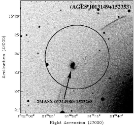
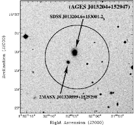
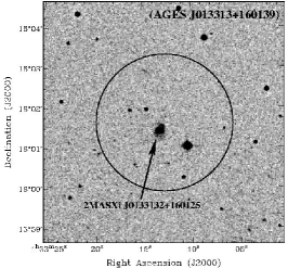
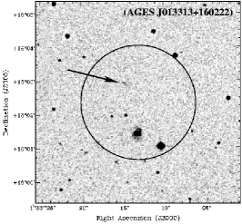
Figure 15: Top to bottom: B band images and accompanying H i spectra for AGES objects J013149+152353, J013204+152947, J013313+160139, J013313+160222

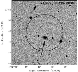
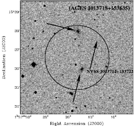
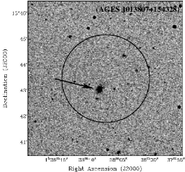
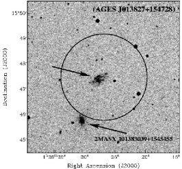
Figure 16: continued

Top to bottom: B band images and accompanying H i spectra for objects J013538+154850, J013718+153635, J013807+154328, and J013827+154728

Top to bottom: B band images and accompanying H i spectra for objects J013917+154613, J013953+151955, J013956+153135 and J014013+153319

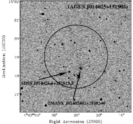
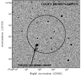
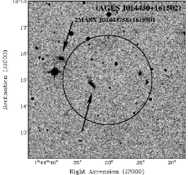
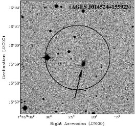
Figure 18: continued

Top to bottom: B band images and accompanying H i spectra for objects J014025+151903, J014033+160513, J014430+161502 and J014524+155923

Top to bottom: B band images and accompanying H i spectra for objects J014630+154332, J014644+155622, J014719+155603 and J014742+161317

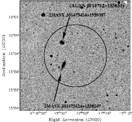
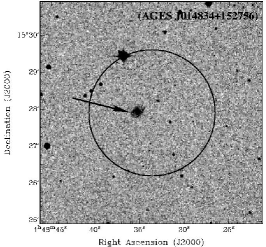
Figure 20: continued

Top to bottom: B band images and accompanying H i spectra for objects J014752+014752 and J014834+152756

There are a further 15 objects whose signals were considered too marginal (S/N $\la 3\sigma$ and $\Delta v<$ 30 km s^-1) to be included in this paper pending further follow-up observations from Arecibo and several other large radio telescopes. From the velocity information alone there appear to be four group associations at around 6000, 8000, 12500 and 16000 km s^-1. J013149+152353 is the one exception being the only galaxy that has no other neighbour within 1700 km s^-1. Fig. 21 is a 3D plot of the galaxies, position and redshift. From this it is possible to distinguish 3 groups: 1 group at $\sim$5000 km s^-1, one at $\sim$8000 km s^-1 and one at $\sim$17000 km s^-1. The objects at $\sim$12500 km s^-1 seem too scattered in RA to be considered a group, although they may be the massive tracers of a filament running at right-angles to our line of sight at this velocity.

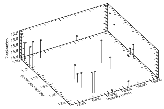
Figure 21: A 3D plot of the positions of the galaxies beyond the NGC 628 group with their H i redshifts.

4.2 Detection efficiency

The precursor survey covered an area of about 4.6 sq.deg. with an rms noise of 1.1 mJy (for 10 km s^-1 resolution) and another 0.9 sq.deg. with an rms noise of 1.8 mJy. Using these noise values we tested the distribution of detections beyond the NGC 628 group using a $V/V_{max}$ test following the procedures described in greater detail by Rosenberg & Schneider (2002). Assuming the line-width dependence for detections that they found along with a roll-off in completeness near the detection limit, the expected mean value of $V/V_{max}$ should be 0.61. By adjusting the signal-to-noise level at which there is a 50% completeness in the detection rate, we found that at an effective S/N = 7 (for a source of 300 km s^-1 line width), the correct value of $V/V_{max}$ was recovered. This sensitivity level is very similar to those derived from $V/V_{max}$ tests of past blind H i surveys.

Given these sensitivity estimates, we modelled the predicted number of sources that should be detected within the precursor survey volume. This analysis is complicated by the fact that the precursor survey covered an area centred on a known group with a substantial void region behind it. We populated the volume with galaxies based on the HIMF derived from an analysis of the Parkes data (Zwaan et al. 2003) down to an H i mass of $3\times 10^{6}$M_⊙. The model galaxies were given rotation speeds consistent with the range normally observed for their H i mass, and then given a random orientation as well as a standard deviation of 300 km s^-1 relative to the Hubble flow. We then ‘observed’ the volume at the measured sensitivity and completeness levels of the survey and determined which galaxies would be detected, repeating this process 1000 times to estimate the likely number of galaxies we should detect.

Based on the Parkes HIMF function we would have expected to detect 49.2$\pm$6.8 galaxies in total. This is almost twice as high as the actual number detected, 27, but only about 3$\sigma$ from the predicted number. Since the nearby volume contains both a known group and a void, we can look instead at the results for the more distant portion of the volume—indeed no galaxies were detected with velocities between that of the NGC 628 group and $cz=4890$ km s^-1. If we consider the volume beyond 4500 km s^-1, where we might anticipate that the volume is relatively unbiased by local large scale structure, the predicted number of detections is 42.3$\pm$6.3. This is again about 3$\sigma$ more than the number detected in this volume, 22.

The predicted number of sources for the Parkes HIMF is higher than would be predicted with most other mass functions because of the relatively high normalisation factor ($\Phi_{\star}=0.0086$ Mpc^-3), which indicates the relative number of galaxies near the ‘knee’ in the mass function at log(M_HI⋆/M_⊙) = 9.79. Both the HIMFs of Rosenberg & Schneider (2002) and Zwaan et al. (1997) have lower normalisation factors yielding a predicted number of detections of 37.2$\pm$6.2 and 28.4$\pm$5.3 respectively. Given the limited area covered by the precursor study, this result may indicate more about cosmic variance than about the HIMF. It should also be noted that because of the relatively low sensitivity of the Parkes survey, its results are based on a relatively nearby volume of space. The full AGES survey will provide a much larger and deeper volume for testing the variance of the HIMF.

4.3 $H$-band properties

In order to preform a preliminary study of the stellar properties of our H i selected sample we use the 2MASS (Skrutskie et al. 2006) data available for the candidate NIR counterparts listed in Table 3. The near infrared data are ideal for this kind of analysis since they are less affected by extinction and they are a good indicator of stellar mass (Gavazzi et al. 1996; Rosenberg, Schneider & Posson-Brown 2005).

2MASS data (extracted from the extended source catalogue) were available for only 15 candidate counterparts of our 27 H i sources. Fig. 22 shows the distribution of the M${}_{HI}/L_{H}$ ratio, of the $H$-band effective radius ($r_{e}$: the radius containing 50% of the light), effective surface brightness ($\mu_{e}$: the mean surface brightness within $r_{e}$) and concentration index ($C_{31}$: the ratio of the radii containing 75% and 25% of the light.) for our sample. As a reference, Fig. 23 shows the same distribution for a sample of 114 galaxies belonging to the HIPASS equatorial strip (Garcia-Appadoo, 2005). The two samples occupy a similar parameter space being composed by ‘normal’ disk-like gas-rich galaxies. Any deeper analysis of the stellar content of the H i sources must be postponed to future works due to the lack of sufficiently deep near infrared and optical data. We only point out that the distribution of the $M_{HI}/L_{H}$ ratio shown in Fig. 22 has to be considered as a lower limit of the real distribution of AGES sources, since it is based on the 15 brightest $H$-band candidate counterparts in our sample.

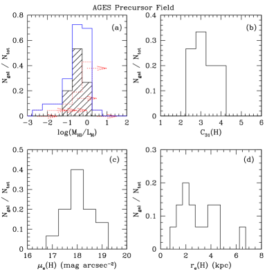
Figure 22: AGES precursor sample H i–$H$-band properties. (a) M${}_{HI}/$L_H distribution. The shaded region represents measured values, the dotted lines represent estimated lower limits for those galaxies that were not detected in $H$-band. The white region is the sum of the measured values and the estimated values. (b) $H$-band concentration parameter distribution. Bulge galaxies are those galaxies with a value greater than 4. (c) $H$-band effective surface brightness distribution. (d) $H$-band effective radius.

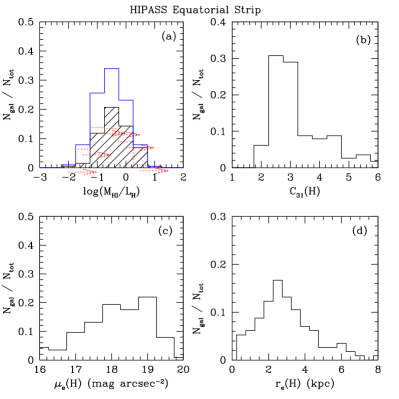
Figure 23: HIPASS Equatorial Strip H i–$H$-band properties. (a) M${}_{HI}/$L_H distribution. The shaded region represents measured values, the dotted lines represent estimated lower limits for those galaxies that were not detected in $H$-band. The white region is the sum of the measured values and the estimated values. (b) $H$-band concentration parameter distribution. Bulge galaxies are those galaxies with a value greater than 4. (c) $H$-band effective surface brightness distribution. (d) $H$-band effective radius.

5 Conclusions

The precursor observations of NGC 628 and its companions have shown that the observing strategy and the data reduction pipeline are all working successfully. The detection rate is close to what we would expect for this volume. With 192s integration time it has been possible to reach a column density limit of 2$\times 10^{18}$cm^-2. Studying the NGC 628 group has revealed no intergalactic gas down to this column density limit.

The detection of dw0137+1541 has shown that the survey is sensitive to low mass H i objects. We have also demonstrated the ability of AGES to detect galaxies out to a velocity of 17500 km s^-1. 3 groups have been identified beyond the NGC 628 group. Of the 22 detections outside of the NGC 628 group, 9 are new detections and 3 galaxies with redshift data available from SDSS compare well with the H i redshifts. 15 low signal-noise detections have also been identified and we have applied for time at several large radio telescopes for follow-up observations to confirm these sources.

From the point of dark galaxy detection, superCOSMOS images have revealed that there is an optical detection within each H i beam, but these objects cannot be assumed to be associated with the H i emission on grounds of spatial coincidence alone. Optical redshift data, and possibly higher resolution H i observations will be required to confirm the associations. To this end we are applying for follow-up observations on several other telescopes.

One of the project goals is to study the HIMF in different environments. With only 27 objects this sample, is much too small to perform any meaningful analysis of the HIMF. However, we have shown that the quality of this data is good enough that the galaxies can be included with those from future AGES fields to compile a HIMF.

References

- (1) Barnes D. G. et al., 2001, Mon. Not. R. Astr. Soc., 322, 486
- (2) Bernardi M. et al., 2003, Astron. J., 125, 1817
- (3) Binggeli B., Tammann G. A., Sandage A., 1987, Astron. J., 94, 251
- (4) Binggeli B., Popescu C. C., Tammann G. A., 1993, Astr. Astrophys. Suppl., 98, 275
- (5) Briggs F. H., 1986, Astrophys. J., 300, 613
- (6) Buckley M. W., Flint K., Impey C. D., Bolte M., 2003, American Astronomical Society Meeting Abstracts, 203,
- (7) Condon J. J., Cotton W. D., Greisen E. W., Yin Q. F., Perley R. A., Taylor G. B., Broderick J. J., 1998, Astron. J., 115, 1693
- (8) Davies J. I., de Blok W. J. G., Smith R. M., Kambas A., Sabatini S., Linder S. M., Salehi-Reyhani S. A., 2001, Mon. Not. R. Astr. Soc., 328, 1151
- (9) Davies J. et al., 2004, Mon. Not. R. Astr. Soc., 349, 922
- (10) de Vaucouleurs G., de Vaucouleurs A., Corwin H. G., Buta R. J., Paturel G., Fouque P., 1991, Third Reference Catalogue of Bright Galaxies. Volume 1-3, XII, 2069 pp. 7 figs.. Springer-Verlag Berlin Heidelberg New York
- (11) Garcia-Appadoo D. A., 2005, PhD thesis, Cardiff University
- (12) Gavazzi G., Pierini D., Boselli A., 1996, Astron. Astrophys., 312, 397
- (13) Gavazzi G., Boselli A., Mayer L., Iglesias-Paramo J., Vílchez J. M., Carrasco L., 2001, Astrophys. J. Letters, 563, L23
- (14) Giovanelli R. et al., 2005, Astron. J., 130, 2598
- (15) Hendry M. A. et al., 2005, Mon. Not. R. Astr. Soc., 359, 906
- (16) Huchra J. P., Vogeley M. S., Geller M. J., 1999, Astrophys. J. Suppl., 121, 287
- (17) Huchtmeier W. K., Karachentsev I. D., Karachentseva V. E., 2003, Astron. Astrophys., 401, 483
- (18) Kamphuis J., Briggs F., 1992, Astron. Astrophys., 253, 335
- (19) Karachentsev I., Musella I., Grimaldi A., 1996, Astron. Astrophys., 310, 722
- (20) Kilborn K., Webster R. L., Staveley-Smith L., 1999, Publs. Astr. Soc. Aust., 16, 8
- (21) Koribalski B. S. et al., 2004, Astron. J., 128, 16
- (22) Lang R. H. et al., 2003, Mon. Not. R. Astr. Soc., 342, 738
- (23) Martin D. C. et al., 2005, Astrophys. J. Letters, 619, L1
- (24) Meyer M. J. et al., 2004, Mon. Not. R. Astr. Soc., 350, 1195
- (25) Mihos J. C., Harding P., Feldmeier J., Morrison H., 2005, Astrophys. J. Letters, 631, L41
- (26) Minchin R. F. et al., 2003, Mon. Not. R. Astr. Soc., 346, 787
- (27) Osmond J. P. F., Ponman T. J., Finoguenov A., 2004, Mon. Not. R. Astr. Soc., 355, 11
- (28) Pisano D. J., Wakker B. P., Wilcots E. M., Fabian D., 2004, Astron. J., 127, 199
- (29) Putman M. E. et al., 2002, Astron. J., 123, 873
- (30) Putman M. E., Staveley-Smith L., Freeman K. C., Gibson B. K., Barnes D. G., 2003, Astrophys. J., 586, 170
- (31) Rosenberg J. L., Schneider S. E., 2002, Astrophys. J., 567, 247
- (32) Rosenberg J. L., Schneider S. E., Posson-Brown J., 2005, Astron. J., 129, 1311
- (33) Ryan-Weber E. V. et al., 2004, Astron. J., 127, 1431
- (34) Ryder S. D. et al., 2001, Astrophys. J., 555, 232
- (35) Sabatini S., Davies J., Scaramella R., Smith R., Baes M., Linder S. M., Roberts S., Testa V., 2003, Mon. Not. R. Astr. Soc., 341, 981
- (36) Sharina M. E., Karachentsev I. D., Tikhonov N. A., 1996, Astr. Astrophys. Suppl., 119, 499
- (37) Skrutskie M. F. et al., 2006, Astron. J., 131, 1163
- (38) Sun M., Murray S. S., 2002, Astrophys. J., 576, 708
- (39) Tully R. B., Fisher J. R., 1987, Nearby galaxies Atlas. Cambridge: University Press, 1987
- (40) Waugh M. et al., 2002, Mon. Not. R. Astr. Soc., 337, 641
- (41) White P. M., Bothun G., Guerrero M. A., West M. J., Barkhouse W. A., 2003, Astrophys. J., 585, 739
- (42) Zwaan M. A., Briggs F. H., Sprayberry D., Sorar E., 1997, Astrophys. J., 490, 173
- (43) Zwaan M. A. et al., 2003, Astron. J., 125, 2842
- (44) Zwaan M. A., Meyer M. J., Staveley-Smith L., Webster R. L., 2005, Mon. Not. R. Astr. Soc., 359, L30