Point Process Algorithm: A New Bayesian Approach for Planet Signal Extraction with the Terrestrial Planet Finder Interferometer

Abstract

The capability of the Terrestrial Planet Finder Interferometer (TPF-I) for planetary signal extraction, including both detection and spectral characterization, can be optimized by taking proper account of instrumental characteristics and astrophysical prior information. We have developed the Point Process Algorithm (PPA), a Bayesian technique for extracting planetary signals using the sine-chopped outputs of a dual nulling interferometer. It is so-called because it represents the system being observed as a set of points in a suitably-defined state space, thus providing a natural way of incorporating our prior knowledge of the compact nature of the targets of interest. It can also incorporate the spatial covariance of the exozodi as prior information which could help mitigate against false detections. Data at multiple wavelengths are used simultaneously, taking into account possible spectral variations of the planetary signals. Input parameters include the RMS measurement noise and the a priori probability of the presence of a planet. The output can be represented as an image of the intensity distribution on the sky, optimized for the detection of point sources. Previous approaches by others to the problem of planet detection for TPF-I have relied on the potentially non-robust identification of peaks in a “dirty” image, usually a correlation map. Tests with synthetic data suggest that the PPA provides greater sensitivity to faint sources than does the standard approach (correlation map $+$ CLEAN), and will be a useful tool for optimizing the design of TPF-I.

1 Introduction

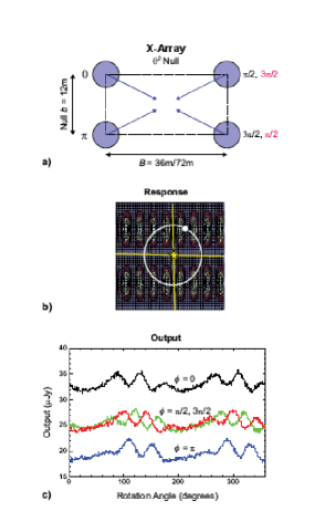
Figure 1: Schematic of Dual-Bracewell Nulling Interferometer array in the X-configuration. (a) Assumed geometry: Two 12 m nulling pairs are separated by 36 m or 72 m. Within each nulling pair, the signals are combined with a relative phase shift of $\pi$, resulting in destructive interference at the location of the star. The signals from the two nulling pairs are then combined coherently after introducing relative phase shifts, alternately, of $\pi/2$ and $3\pi/2$; the difference between these two signals then constitutes the “sine-chop” signal. In practice, the required pair of sine-chop differencing signals is obtained by combining the beams from all four elements simultaneously in a central beam combiner, after introducing a set of phase shifts, to the individual elements, of either $\{0,\pi,\pi/2,3\pi/2\}$ or $\{0,\pi,3\pi/2,\pi/2\}$. (b) Angular response on the sky when combining the two nulled signals with $\pi$ phase shift; the star (nulled out) is at the center, and the planet position is indicated by the white disk. A modulated signal is produced as the interferometer system rotates and the planet passes through peaks and valleys of the response. (c) Example of modulated signals at 12 $\mu$m wavelength simulating an observation of a planet 3 Earth radii in size, 1 AU from a G2 star at 10 pc, using an X-array with $B=36$ m and $b=9$ m.

A key component of the proposed Terrestrial Planet Finder mission is a nulling interferometer (TPF-I) for the wavelength range 7–15 $\mu$m, currently envisaged as a free-flying four-element dual-Bracewell array in the “X” configuration as shown in Figure 1. The signals from the two elements in a nulling pair are combined with $\pi$ phase shift, resulting in destructive interference for a source on the optical axis, i.e., the axis corresponding to equal geometrical path lengths to the two nulling elements. By placing this null at the location of the star, the contrast between planets and star is dramatically increased, thereby overcoming one of the chief obstacles to planet detection (Bracewell, 1978). The starlight suppression is further improved by using two such nulling pairs and combining their outputs coherently (see, for example, Beichman & Velusamy (1999)). As the interferometer system is rotated about the line of sight, a modulated signal is then produced, and this signal contains information on the intensity distribution of sources on the sky. Its information content can be increased by alternately applying phase shifts of $\pi/2$ and $3\pi/2$ and taking the difference of the phase-shifted signals. This has the effect of suppressing instrumental effects such as low-frequency detector noise and thermal background drifts, and is commonly referred to as “sine chopping” ((Woolf et al., 1998; Velusamy & Beichman, 2001)). Sine chopping also suppresses any structure on the sky which is symmetrical about the star, including that from symmetrical structure in the exo-zodiacal (exozodi) cloud, thus increasing the contrast for the detection of planetary signals.

Since the interferometric signals from such a small number of baselines provide very limited information on spatial Fourier components of the intensity distribution of sources on the sky, it is necessary to supplement the observations with a priori information in order to recover that distribution. One widely-used procedure for this purpose is the maximum entropy method (see Narayan & Nityananda (1986) for a review, and Sutton & Wandelt (2006) for recent developments). However, such procedures are not optimal for the present problem because they do not incorporate an important piece of prior knowledge, namely the pointlike nature of the planetary sources.

Of the various inversion procedures that do incorporate such information (see, for example, Angel & Woolf (1997); Velusamy & Marsh (2004)), the one most widely used involves making a correlation map (referred to as a “dirty image”) followed by deconvolution with the CLEAN algorithm (Högbom, 1974; Draper et al., 2005). A key step in that procedure is an iterative search for peaks in the dirty image, which can be non-robust when noise bumps fall on “side lobes” of the responses to other sources.

In this paper we propose a Bayesian technique for planet detection which avoids the noise-vulnerable peak-finding step. It can process data at many wavelengths simultaneously, and can incorporate prior information such as the spatial covariance of the exozodi. Since the planetary signals are represented as a random set of points in a suitably-defined state space, we refer to the resulting algorithm as a “Point Process Algorithm” (PPA) following the terminology of Richardson & Marsh (1992).

The PPA, whose mathematical foundation is presented in detail by Richardson & Marsh (1987), is a general technique of which the TPF problem represents a specific application (Velusamy et al., 2005). It may be regarded as a state estimation technique in which the system to be described (for example, an image) consists of the superposition of an indefinite number of objects, each of which is characterized by a set of parameter values. Each object can thus be represented as a single point in a multidimensional state space of which each axis corresponds to one of the parameter values. In our application, the axes of the state space are simply the $x$ and $y$ positions and flux density of an individual point source. Other possible examples are: (1) the representation of an image of a cluster of galaxies in terms of a 6-dimensional state space in which the axes represent the $x$ and $y$ location, the flux density, major and minor axes and orientation of an individual galaxy, and (2) the representation of a planetary system using a state space whose axes consist of the orbital parameters characterizing an individual planet, using a set of measurements of Doppler shifts or astrometric measurements of the parent star (or both). In each of these examples, the goal of the PPA is to estimate the most probable set of points in the state space given the set of measurements.

2 Measurement Model

The starting point of our approach is a measurement model which relates a data vector, $\mathbf{d}$ (whose components are the complete set of samples of the sine-chop signal at all wavelengths of observation), to the intensity distribution, $I(x,y)$, on the sky. The latter is modeled as the superposition of a set of point sources of unknown number, fluxes and positions, upon an extended background whose intensity at position $\left(x_{j},y_{j}\right)$ is denoted by $\zeta_{j}$. The distribution of point sources is represented as a set of occupation numbers in a 3-dimensional state space whose axes are flux and $x$, $y$ position. The state space is divided into a regularly-sampled grid of cells, such that the cell with coordinates $\left(f_{k},x_{j},y_{j}\right)$ represents the $k$th possible flux value, $f_{k}$, at the $j$th spatial position, $\left(x_{j},y_{j}\right)$. If a point source of that particular flux density is present at that particular position, then the occupation number of that cell, $\Gamma_{n}$ (where indices $j$ and $k$ have been mapped onto a single index, $n$), will be equal to 1; otherwise, it will equal zero. This representation provides a convenient framework within which to incorporate our prior knowledge of spatial dilution.

We assume that the source distribution is being observed by a rotating dual-Bracewell interferometer consisting of two nulling pairs separated by an “imaging baseline,” and that the measurements consist of a time series of sine-chop signal values as the system rotates with respect to the sky. If the $i$th such measurement is made at an orientation corresponding to instantaneous baseline vectors ${\mathbf{b}}_{i}$ and ${\mathbf{B}}_{i}$ for the nulling and imaging baselines respectively, then the instantaneous response to a point source of unit flux at off-axis sky position $(x_{j},y_{j})$ (denoted by unit vector ${\mathbf{s}}_{j}$) is given by:

$$H_{i}(x_{j},y_{j})=-4\sin^{2}(\pi{\mathbf{s}}_{j}\cdot{\mathbf{b}}_{i})\sin(2\pi{\mathbf{s}}_{j}\cdot{\mathbf{B}}_{i})R_{i}({\mathbf{s}}_{j})$$ (1)

where $R_{i}({\mathbf{s}}_{j})$ is the “primary beam” response, i.e., the response of an individual detector, and the baselines ${\mathbf{b}}_{i}$ and ${\mathbf{B}}_{i}$ are in units of wavelengths.

The measurement model must include a spectral model which relates the planetary fluxes at the different wavelengths. There are several possibilities, one of which is to treat the planets as black bodies at the local radiation temperature. If the orbital inclination and position angle of the orbital tilt axis are known, the planet temperature, $T_{j}\equiv T\left(x_{j},y_{j}\right)$, can then be determined at each $\left(x_{j},y_{j}\right)$ from knowledge of the stellar luminosity and radial distance. Our measurement model can then be written as:

$$d_{i}=\sum_{j,k}{f_{k}\left[{B\left(\lambda_{i},T_{j}\right)}/{B\left(\lambda_{0},T_{j}\right)}\right]H_{i}\left(x_{j},y_{j}\right)\Gamma_{n}}+\sum_{j}{H_{i}\left(x_{j},y_{j}\right)\zeta_{j}\left(\lambda_{i}\right)}+\nu_{i}$$ (2)

where $\lambda_{i}$ represents the wavelength at which the $i$th measurement is made, $B\left(\lambda,T\right)$ represents the Planck function, and the $f_{k}$ represent possible values of planetary flux at some suitably-defined reference wavelength, $\lambda_{0}$, and $\nu_{i}$ is the measurement noise. The index, $n$, is understood to be a function of $j$ and $k$.

It will be convenient to lump both of the last two terms on the r.h.s. of (2) into a single “noise” vector, $\mu$, whose components are given by:

$$\mu_{i}=\sum_{j}{H_{i}\left(x_{j},y_{j}\right)\zeta_{j}}+\nu_{i}$$ (3)

If we then define a matrix $\mathbf{A}$ whose components are

$$A_{in}=f_{k}\left[{B\left(\lambda_{i},T_{j}\right)}/{B\left(\lambda_{0},T_{j}\right)}\right]H_{i}\left(x_{j},y_{j}\right)$$ (4)

then we can rewrite (2) in matrix notation as:

$$\mathbf{d}=\mathbf{A}\mathbf{\Gamma}+\mu$$ (5)

where $\mathbf{\Gamma}$ is the state vector whose components are $\Gamma_{n}$.

3 Statistical Assumptions

The measurement noise in the TPF signals is distributed as a Poisson process, dominated by the photon statistics of stellar leakage and the local zodi background. Since the expected number of photons per integration period is large (typically $\sim 10^{5}$), the statistical distribution accurately attains the limit corresponding to a Gaussian random process (GRP). The measurement noise, $\nu_{i}$, on the sine-chop signal can then be regarded as a zero-mean GRP for which:

$$E\nu_{i}\nu_{i^{\prime}}=\left(\sigma_{\nu}\right)_{i}^{2}\delta_{ii^{\prime}}$$ (6)

where $E$ is the expectation operator and $\delta$ is the Kronecker delta.

For present purposes we regard the exozodi as an error source rather than as a quantity to be estimated. We model it only to the extent necessary to mitigate its effects on planet detection. If it is distributed symmetrically about the star, then its only effect is to increase $\sigma_{\nu}$ by a factor corresponding to the square root of the increase in the overall photon count, since its coherent contribution cancels out in the sine chop signal. If the exozodi is not symmetrical, one approach for dealing with it is to subtract its estimated contribution from the measurements ahead of time, based on available data from previous (possibly ground-based) observations at lower resolution. The error resulting from this subtraction may be regarded as an additional zero-mean error contribution to our measurement model. It will, in general, be spatially correlated as a result of the finite resolution of the observations and the intrinsic spatial correlation properties of the exozodi itself. We therefore approximate the residual exozodi, $\zeta_{j}(\lambda_{i})$, as a GRP with covariance $C_{\zeta}$ defined by:

$$E\zeta_{j}\zeta_{j^{\prime}}=\left(C_{\zeta}\right)_{jj^{\prime}}$$ (7)

From (6) and (7), we can then show that the covariance of $\mu$ is given by:

$$\left(C_{\mu}\right)_{ii^{\prime}}\equiv E\mu_{i}\mu_{i^{\prime}}=\sum_{j,j^{\prime}}\left(C_{\zeta}\right)_{jj^{\prime}}H_{i}\left(x_{j},y_{j}\right)H_{i^{\prime}}\left(x_{j^{\prime}},y_{j^{\prime}}\right)+\left(\sigma_{\nu}\right)_{i}^{2}\delta_{ii^{\prime}}$$ (8)

The state vector, $\mathbf{\Gamma}$, is also regarded as a stochastic process; its a priori probability distribution is assumed to be described by:

$$P\left(\mathbf{\Gamma}\right)=\prod_{n}P\left(\Gamma_{n}\right)$$ (9)

where

$$P\left(\Gamma_{n}\right)=\left\{\begin{array}[]{r@{\qquad}l}P_{1}&\mbox{if}~{}~{}\Gamma_{n}=1\\ 1-P_{1}&\mbox{if}~{}~{}\Gamma_{n}=0\\ 0&\mbox{otherwise}\end{array}\right.$$ (10)

The quantity $P_{1}$ thus represents the a priori probability of occupancy of a cell in the state space of flux and position.

4 Estimation Procedure

The central operation is to estimate the state vector, $\mathbf{\Gamma}$, given the observed data. The details of the estimation process depend on the type of optimality criterion selected. For the present algorithm we choose a mean square error criterion, for which the optimal estimate is the a posteriori average value of $\mathbf{\Gamma}$, given by:

$$\rho\left(z_{n}|\mathbf{d}\right)\equiv E\left(\Gamma_{n}|\mathbf{d}\right)=\sum_{\mathbf{\Gamma}}\Gamma_{n}P\left(\mathbf{\Gamma}|\mathbf{d}\right)$$ (11)

where $z_{n}$ is a 3-d vector representing the coordinates, $(x_{j},y_{j},f_{k})$, of the $n$th cell in state space, and the conditional probability, $P(\mathbf{\Gamma}|\mathbf{d})$, is given by Bayes’ rule:

$$P\left({\mathbf{\Gamma}}|\mathbf{d}\right)=P\left(\mathbf{d}|\mathbf{\Gamma}\right)P(\mathbf{\Gamma})/P(\mathbf{d})$$ (12)

in which $P({\mathbf{\Gamma}})$ is given by (9), $P(\mathbf{d})$ is a normalization constant, and

$$\ln P\left(\mathbf{d}|\mathbf{\Gamma}\right)=-\frac{1}{2}(\mathbf{d}-\mathbf{A\Gamma})^{\mbox{\scriptsize{T}}}\mathbf{C}_{\mu}^{-1}(\mathbf{d}-\mathbf{A\Gamma})+{\rm const.}$$ (13)

We refer to $\rho\left(z_{n}|\mathbf{d}\right)$ as a density, since it represents the average local density of occupied cells in the state space of position and flux. Its estimation is a generic problem in statistical mechanics; previous applications have included acoustical imaging (Richardson & Marsh, 1987) and target tracking (Richardson & Marsh, 1992). The solution procedure involves the solution of a hierarchy of integro-differential equations which fortunately can be truncated, to a good approximation, at the first member. We then obtain:

$$\frac{\partial\rho}{\partial t}+\phi_{1}\rho=0$$ (14)

where $t$ is a dimensionless progress variable representing the degree of conditioning on the data, and $\phi_{1}$ is the conditioning factor given by:

$$\phi_{1}=-\left(\mathbf{d}-\mathbf{A}\rho\right)^{\mbox{\scriptsize{T}}}\mathbf{C}_{\mu}^{-1}\mathbf{A}+\mathbf{b}/2$$ (15)

where $\mathbf{b}$ represents a vector formed from the diagonal elements of $\mathbf{A}^{\mbox{\scriptsize{T}}}\mathbf{C}_{\mu}^{-1}\mathbf{A}$. A discretized version of (14) is formed by regarding the process as a series of $N_{\rm c}$ weak conditionings, each of which corresponds to a measurement noise covariance of $N_{\rm c}\mathbf{C}_{\mu}$. The progress variable, $t$, then corresponds to the number of conditionings, and the $dt$ in (14) is replaced by 1. Equation (14) is then to be integrated from $t=0$ to a terminal value, $t_{f}=N_{\rm c}$, representing full conditioning on the data.

The initial condition on $\rho$ for the numerical solution of (14) is $\rho_{(t=0)}=\rho_{0}$, where $\rho_{0}$ is the a priori density equal to the constant value $P_{1}$; its sum over all state space is equal to $N_{0}$, the a priori expectation number of planets present. If we regard the true number of planets, $N$, as an unknown, then this quantity could, in principle, be estimated by adjusting $P_{1}$ for equality between $N_{0}$ and the a posteriori number of planets, corresponding to the sum of $\rho(z_{n}|\mathbf{d})$ over all state space (Richardson & Marsh, 1987). In practice, however, this would be numerically cumbersome. We have therefore adopted an approximate alternate procedure in which the number of planets is estimated with the aid of $\chi_{\nu}^{2}$, given by:

$$\chi_{\nu}^{2}=\frac{1}{M}\sum_{i}\left(\mathbf{d}-\mathbf{A}\rho\right)_{i}^{2}/\left(C_{\mu}\right)_{ii}$$ (16)

where $M$ is the total number of data samples. In this procedure, we fix $P_{1}$ at a very small value, thereby producing an a priori bias towards a small number of planets being present. We then proceed with the numerical integration (during the course of which, $\chi_{\nu}^{2}$ decreases monotonically), terminating it when $\chi_{\nu}^{2}=1$. We thereby arrive at a solution in which the data are fit by the minimum possible number of planets.

Our corresponding estimate of the source intensity distribution is then:

$$\hat{I}\left(x_{j},y_{j}\right)=\sum_{k}f_{k}\rho\left(z_{n(j,k)}|\mathbf{d}\right)$$ (17)

Estimates of the planet fluxes themselves may be obtained from the integrated value around each peak in this image; the uncertainties correspond to the standard a posteriori variances of maximum likelihood estimates.

5 Tests with Synthetic Data

We have tested the PPA using a set of 15 test cases designed to replicate realistic observing scenarios for TPF-I in the wavelength range 7–15 $\mu$m. Each case involved 0–5 planets at radial distances of 0.4–5.25 AU from a solar-type star at a distance of 10 or 15 pc, superposed on a 1 Zodi dust distribution. The 15 cases involved a total of 37 planets, 24 of which were of 1 Earth flux, and 2 of which were $<1$ Earth flux. The orbital inclination was $60^{\circ}$ except for two face-on cases. All planets were at Earth temperature (260 K). Radial distances and signal-to-noise ratios were distributed as shown in Figure 2.

The measurement configuration was the “X array” consisting of four 4-m detectors at the vertices of a rectangle of width 12 m (corresponding to the nulling baseline length) and a length of either 36 m or 72 m, as shown in Figure 1. We adopted the 12 m nulling baseline in lieu of the nominal design value of 20 m to improve the sensitivity at the short wavelengths. For longer baselines (20 m in particular), the stellar leakage becomes larger because of the narrower null, with particularly severe effects at the shorter wavelengths.

The measurements consisted of the simulated sine chop signals through a full rotation of the array, at wavelengths of 7.44, 8.50, 9.92, 11.90 & 14.90 $\mu$m, with bandwidths ranging from 0.9 $\mu$m at 7.44 $\mu$m to 3.7 $\mu$m at 14.9 $\mu$m, and a total integration time of 1 day. Superposed on these signals was Poisson noise due to the various instrumental and astrophysical effects discussed by Beichman & Velusamy (1999), the most important ones being stellar leakage (due to incomplete nulling of the stellar photosphere) and thermal emission from the local- and exo-zodiacal dust clouds, the latter assumed geometrically symmetrical.

The data were inverted using the PPA, and also by the standard technique of “correlation map + CLEAN” for comparison purposes. The spatial covariance of the exozodi was ignored (i.e., $C_{\zeta}$ was set at zero) since symmetrical sources cancel in the sine chop signal. Full account was, however, taken of the Poisson noise contribution of this component. Figure 3 shows the results for five representative cases involving both array configurations. The results of the PPA and CLEAN algorithms are shown for the 36 m and 72 m configurations; note that in the case of CLEAN, only the 6 strongest source components are shown. Also shown (Column 4) is the result of using the PPA with a combination of data from both configurations, but with the integration time split equally between the two, i.e., the integration time was 0.5 day per configuration.

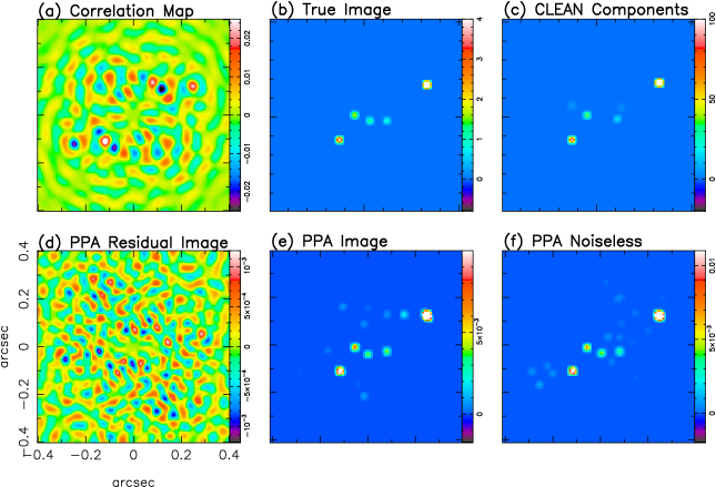
Figure 4: Images obtained by PPA and CLEAN methods for a test case involving 5 planets with the X-36m array. Similar images were obtained for all 15 test cases.

Figure 4 shows the results for the case involving 5 assumed planets (Case 4 of the previous figure). Also shown for comparison (panel (e) of Figure 4) is the result of using noiseless data; it demonstrates that the fidelity of the PPA image is limited, in part, by the gaps in spatial frequency coverage of the measurements.

For all 15 test cases, these inversions yielded images from which we extracted estimates of point source locations, fluxes, and corresponding uncertainties. We identified the six brightest peaks in each image, then applied a SNR threshold and counted the detections. Comparison with the true (assumed) planet positions then led to the number of true detections and false alarms as a function of the detection threshold in sigmas. The fluxes of detected sources were recovered to an accuracy consistent with their theoretical uncertainties. For the 5-planet case above, with the 36 m array, these uncertainties ranged from approximately 2% for the brightest source (8 Earth fluxes) to 20% for the weakest (1 Earth flux).

Figure 5 shows a plot of true positives vs. false negatives, known as the operating characteristic curve of the detection system, for both PPA and CLEAN. Also included in the figure is the theoretical operating characteristic curve for an isolated source observed with the 36-m array, assuming pure Gaussian statistics. It is apparent that the PPA detected significantly more planets than CLEAN, particularly in the case of the fainter objects at low $S/N$ thresholds. While it is also apparent that the PPA results fall below the theoretical curve, it should be borne in mind that the latter did not take into account the interactions between sources due to the incomplete spatial frequency coverage. Figure 6 shows the PPA performance as a function of detection threshold in sigmas for the 36-m array.

6 Discussion

The PPA is theoretically a near-optimal approach, and the present results support this. They demonstrate that use of the PPA increases the effective sensitivity for planet detection over standard techniques exemplified by CLEAN.

The results also indicate that the 72 m array would be less sensitive than the 36 m array for this ensemble of planets, presumably due to the smaller relative range of spatial frequencies involved. For this reason, it would be more effective, for a given amount of integration time, to use the 36 m array exclusively rather than split the time between the 36 m and 72 m configurations, even though the inclusion of the 72 m array would increase the overall spatial frequency coverage. The fact that this added coverage did not offset the reduced integration time of the 36 m array is apparent from the results in Figure 3, and is confirmed by the statistical results from the complete set of 15 cases.

Future work in the application of the PPA to the planet detection problem will emphasize the effects of exozodi, including the effects of spatial inhomogeneities which may masquerade as planets in the interferometer signals, and their mitigation via appropriate incorporation of a priori estimates and spatial covariance. For the latter purpose we will make use of recent observations of debris disks using the Spitzer Space Telescope (Beichman et al., 2005).

We will also explore some of the possible applications of the PPA beyond the TPF problem, since, as we have discussed, it is not limited to the detection of point sources. It may, in fact, be regarded as a generic technique for modeling a set of data (which may or may not be image-like) in terms of user-defined primitives (i.e., objects) which are parametrizable. The main requirement is that the superposition rule be satisfied, i.e. that the measurements represent a linear combination of the contributions from the individual objects in the system. The objects themselves need not be defined in terms of astrophysical entities; they may instead be a set of parametrizable fractal elements convenient for representing an observed image. In such an application, the goal of the PPA would be similar to that of adaptive scale pixel deconvolution techniques such as the Asp-CLEAN technique of Bhatnagar & Cornwell (2004) and the “pixon” technique (Dixon et al., 1996). Unlike the latter, however, the PPA is not restricted to cases involving PSFs of finite support, and it has some potential advantages over the former. One of these is that it may provide a more efficient procedure for spatially-complex images, since a consequence of the PPA’s use of an occupation-number representation is that the computational burden does not increase significantly with the number of source components in the image. The second potential advantage of the PPA is that it is fully capable of superresolution, which in practical terms means that it can separate adjacent point sources whose separation is less than the PSF width. It is not clear that Asp-CLEAN would have this capability given the fact that the standard CLEAN algorithm does not. We will investigate these and other issues in order to better characterize PPA’s niche in astronomical problems.

Figure 2: The distribution of planet parameters in the test cases, with respect to radial distance from the star and corresponding ideal SNR for an isolated planet. The distances to the stars are as indicated.

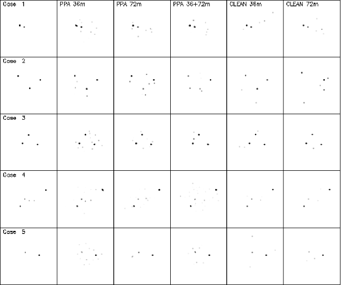
Figure 3: Five representative cases, showing the results for PPA and CLEAN with two configurations of the interferometer. The true intensity distributions are shown in the left hand column. Columns 2 and 3 show the results of the PPA for the 36 m and 72 m arrays, respectively, for an total integration time of 1 day. Column 4 shows the results of the PPA using data from both configurations combined, but with the same total integration time, i.e., a half-day per configuration. Columns 5 and 6 give the results obtained using CLEAN for the 36 m and 72 m arrays, showing the 6 strongest source components in each case.

Figure 5: Planet detection statistics, showing the operating characteristic curves for PPA and CLEAN. The solid line on the left hand plot represents the idealized theoretical curve for an isolated planet.

Figure 6: Detection performance of PPA with the 36-m array as a function of threshold in sigmas.

References

- Angel & Woolf (1997) Angel, J. R. P. & Woolf, N. J. 1997, ApJ, 475, 373
- Beichman et al. (2005) Beichman, C. A. et al. 2005, ApJ, 622, 1160
- Beichman & Velusamy (1999) Beichman, C. A. & Velusamy, T. 1999 in: S. C. Unwin & R. V. Stachnick (eds.), Optical & IR Interferometry from Ground and Space (ASP Conference Series) Vol. 194, pp 405–419
- Bhatnagar & Cornwell (2004) Bhatnagar, S. & Cornwell, T. J. 2004, A&A, 426, 747
- Bracewell (1978) Bracewell, R. N., 1978, Nature, 274, 780
- Dixon et al. (1996) Dixon, D. D. et al. 2006, A&AS, 120, 683
- Draper et al. (2005) Draper, D. W. et al. 2005, AJ, submitted
- Högbom (1974) Högbom, J. A. 1974, A&AS, 15,417
- Narayan & Nityananda (1986) Narayan, R. & Nityananda, R. 1986, ARA&A, 24, 127
- Richardson & Marsh (1987) Richardson, J. M. & Marsh, K. A. 1987, Acoustical Imaging, 15, 615
- Richardson & Marsh (1992) Richardson, J. M. & Marsh, K. A. 1992, in: C. R. Smith et al. (eds.), Maximum Entropy and Bayesian Methods (Kluwer Academic Publishers, Netherlands), pp 213–220
- Sutton & Wandelt (2006) Sutton, E. C. & Wandelt, B. D. 2006, ApJS, 162, 401
- Velusamy & Beichman (2001) Velusamy, T. & Beichman, C. A. 2001, IEEE Aerospace Conference Proceedings Vol 4, p 2013
- Velusamy & Marsh (2004) Velusamy, T. & Marsh, K. A. 2004, Proceedings of 2nd TPF/Darwin International Conference (Dust Disks and the Formation, Detection and Evolution of Habitable Planets) San Diego, July 28–29, 2004
- Velusamy et al. (2005) Velusamy, T., Marsh, K. A., Ware, B. 2005, “Point Process Algorithm: A New Bayesian Approach for TPF-I Planet Signal Extraction,” in C. Aime & F. Vakili, eds., Proceedings of IAU Colloquium No. 200, “Direct Imaging of Exoplanets: Science & Techniques,” Cambridge University Press
- Woolf et al. (1998) Woolf, N. J. et al. 1998, Proc. SPIE 3350, Astronomical Interferometry, R. D. Reasenberg, ed., 683