The Metal-Strong Damped Ly$\alpha$ Systems

Abstract

We have identified a metal-strong (log${N({\rm Zn^{+}})}\geq 13.15$ or log${N({\rm Si^{+}})}\geq 15.95$) DLA (MSDLA) population from an automated quasar (QSO) absorber search in the Sloan Digital Sky Survey Data Release 3 (SDSS-DR3) quasar sample, and find that MSDLAs comprise $\approx 5\%$ of the entire DLA population with $z_{abs}\geq 2.2$ found in QSO sightlines with $r<19.5$. We have also acquired 27 Keck ESI follow-up spectra of metal-strong candidates to evaluate our automated technique and examine the MSDLA candidates at higher resolution. We demonstrate that the rest equivalent widths of strong Zn II $\lambda$2026 and Si II $\lambda$1808 lines in low-resolution SDSS spectra are accurate metal-strong indicators for higher-resolution spectra, and predict the observed equivalent widths $W_{obs}$ and signal-to-noise ratios (SNRs) needed to detect certain extremely weak lines with high-resolution instruments. We investigate how the MSDLAs may affect previous studies concerning a dust-obscuration bias and the ${N({\rm HI})}$-weighted cosmic mean metallicity $<Z(z)>$. Finally, we include a brief discussion of abundance ratios in our ESI sample and find that underlying mostly Type II supernovae enrichment are differential depletion effects due to dust (and in a few cases quite strong); we present here a handful of new Ti and Mn measurements, both of which are useful probes of depletion in DLAs. Future papers will present detailed examinations of particularly metal-strong DLAs from high-resolution KeckI/HIRES and VLT/UVES spectra.

Accepted to the PASP: July 12, 2006

1 Introduction

Damped Ly$\alpha$ systems (DLAs) are the subset of quasar absorption line (QAL) systems classically defined to have neutral hydrogen column densities $N_{\rm HI}\geq 2\times 10^{20}$ atoms cm^-2 (Wolfe, Gawiser & Prochaska, 2005). They are identified by their wide damped Ly$\alpha$ absorption profiles, and all DLAs (to date) show associated metal-line absorption (Prochaska et al., 2003). DLAs dominate the neutral gas content of the universe and may be expected to constitute the primary reservoir of star-forming gas at high redshift (Wolfe et al. 1995; Prochaska and Herbert-Fort 2004; Prochaska, Herbert-Fort and Wolfe 2005, hereafter PHW05). Therefore, measurements of DLA chemical abundances at high redshift help quantify the chemical evolution of the young universe.

Echelle observations of DLAs allow one to accurately measure the gas-phase abundances of a number of elements and thereby examine processes of nucleosynthetic enrichment and differential depletion in these galaxies (e.g. Lu et al., 1996; Vladilo et al., 2001; Prochaska & Wolfe, 2002; Dessauges-Zavadsky et al., 2003). However, Pettini et al. (1994) showed that high-redshift DLAs are generally metal-poor. Their results and subsequent studies (Pettini, 1999; Prochaska et al., 2003; Kulkarni et al., 2005) have tracked the enrichment of the ISM of galaxies reaching back to the first few Gyr. The majority of DLAs show detections of Fe II, Ni II, Si II, and Al II transitions. It is unfortunate that the signatures of Type II SNe enrichment (Woosley & Weaver, 1995) and differential depletion (e.g. Savage & Sembach, 1996) are nearly degenerate for this small set of elements. As such, progress in interpreting the gas-phase abundance patterns of the damped Ly$\alpha$ systems has been difficult, although recent works on S, Zn, N and O have made advances.

Prochaska, Howk, and Wolfe (2003) reported the discovery of a metal-strong DLA at $z_{abs}=2.626$ towards the quasar FJ0812+32 (hereafter DLA-B/FJ0812+32). In contrast with the majority of damped Ly$\alpha$ systems, the authors detected over 20 elements in this single DLA system and revealed the detailed chemical enrichment pattern of this galaxy. Many of the detected transitions had never before been observed outside of the Local Group and are important diagnostics to theories of nucleosynthesis and galaxy enrichment. The authors suggested that this system was enriched mainly by short-lived, massive stars and that it is the progenitor of a massive elliptical galaxy (see also Fenner, Prochaska, & Gibson, 2004). The goal of this work is to speed the discovery and analysis of more systems like DLA-B/FJ0812+32; these rare DLAs are unique laboratories for the study of nucleosynthesis, galaxy enrichment, dust depletion, and ISM physics in the high-redshift universe. We hereafter refer to this special subset of DLA as the metal-strong DLA (MSDLA) systems.

Whilst our primary motivation for defining MSDLAs as those absorbers with high metal column densities (see $\S$ 2), we note that our definition also corresponds to an empirical upper bound to ${N({\rm Zn^{+}})}$ noted by Boissé et al. (1998) for a sample of DLAs in the literature at that time. Boissé et al. interpreted the upper bound to ${N({\rm Zn^{+}})}$ as a selection bias related to dust obscuration (i.e. very large dust-to-gas ratio). However, our statistics on MSDLAs (in sightlines with $r<19.5$) now lead us to argue that the paucity of high N(Zn) absorbers is not due to dust, but simply an indication of their intrinsic rarity (see also Johansson & Efstathiou 2006).

We will show that only a few percent of all DLAs are truly metal-strong, and so thousands of quasar sightlines must be searched in order to discover just a handful of MSDLAs. Therefore, automated detection algorithms used on large quasar surveys are critical to metal-strong DLA research. This paper presents our automated method of detecting metal-strong absorbers in low-resolution Sloan Digital Sky Survey (SDSS) quasar spectra. We detail and release our search algorithms and present all of the metal-strong candidates from SDSS Data Release Three (SDSS-DR3; Abazajian et al., 2005).

As mentioned above, the elemental abundances from DLAs can be used to constrain and test processes of nucleosynthesis. For example, there are several different theories on the production of Boron. Woosley et al. (1990) suggested that B production results from neutrino spallation in the carbon shells of SNe, while Cassé et al. (1995) have argued for the spallation of C and O nuclei accelerated by SNe onto local interstellar gas. Other theories involve protons and neutrons being accelerated onto interstellar CNO seed nuclei, and each theory predicts how B may scale with the galaxy’s metallicity (and so here, for example, one must eventually acquire ${N({\rm HI})}$, although it is not necessary for the project at hand). Measurements of such elements in DLA systems can thus help distinguish between the various theories. Other elements measured in the Galactic ISM would also impact our understanding of nucleosynthesis and star formation in young galaxies if these elements were observed in high redshift DLA. These include: (1) O – an unambiguous $\alpha$-element and the most abundant metal in the universe; (2) Sn and Kr – r-process elements (rapid neutron capture in high density and temperature regions); and (3) Pb – an s-process element (slow neutron decay and capture in low density and temperature regions). Unfortunately, these elements are rarely detected in typical DLA spectra because they have small absolute abundances and/or their dominant ions have transitions with either too large or small oscillator strengths (e.g. O I $\lambda\lambda 1302,1355$). In MSDLAs, however, weaker transitions become available, allowing high-redshift studies of the processes mentioned above.

To gauge the success rate of our algorithms, we have obtained moderate-resolution follow-up observations of a subset of the SDSS-DR3 MSDLA candidates with the
Echelle Spectrograph and Imager (Sheinis et al., 2002, ESI) on the 10m-class Keck II telescope. We present our ESI spectra of 27 MSDLA candidates ($1.6\leq z_{abs}\leq 3.1$ and $r<19.5$) and discuss the implications of this candidate metal-strong subsample.

We define the MSDLAs and discuss the impact of Ly$\alpha$ on our study in $\S$ 2, present our automated technique for detecting metal-strong systems in SDSS, describe how we compiled our sample for medium-resolution observations, and report our SDSS search success rates in $\S$ 3. Section 4 gives a summary of our ESI follow-up observations, data reduction, and measurements. $\S$ 5 presents our analysis and discussion of metal-strong indicators in SDSS QSOs, using our ESI sample as a reference. Section 6 derives our predictions for detecting certain extremely weak lines with HIRES. Section 7 discusses our metal-strong sample and its relation to the proposed dust-obscuration bias, as well as a preliminary investigation of how this MSDLA population might influence previous detections of an evolution in the $N_{\rm HI}$-weighted cosmic mean metallicity $<Z(z)>$. Section 8 concludes the discussion with a few abundance ratios from our ESI data with comments on SNe enrichment and depletion due to dust, and our summary and conclusions are blended together in $\S$ 9.

2 MSDLA Definition and the Impact of Ly$\alpha$

With this paper we define the metal-strong DLAs (MSDLAs) to have log${N({\rm Zn^{+}})}\geq 13.15$ or log${N({\rm Si^{+}})}\geq 15.95$, based on the Zn II and Si II transitions measured in
KeckI/HIRES data of DLA-B/FJ0812+32. These values are somewhat arbitrary, but chosen because they imply equivalent widths for weak transitions like B II 1362 that can be detected with current 10m-class telescopes. We have specifically chosen to define the MSDLA subset based on column density thresholds and not metallicity (ie. not [Zn/H] or [Si/H]), due to motivations from the DLA-B/FJ0812+32 study. Specifically, we aim to discover systems which may be used as high-redshift probes of the production of elements like B, O and Ge (among others) independent of the $N_{\rm HI}$ value. Therefore, we do not require having Ly$\alpha$ measurements and corresponding metallicities (ie. for targeting metal-strong systems), although having $N_{\rm HI}$ will eventually allow the calculations of ionization fractions and dust-to-gas ratios. We caution that choosing a metal column density threshold leads to a mixture of high-$N_{\rm HI}$, low-metallicity, and low-$N_{\rm HI}$, high-metallicity systems which may be very different in their properties. This may affect our conclusions about the nature or evolution of the metal-strong systems. We will address these issues in more detail with future papers on high-resolution metal-line observations complete with $N_{\rm HI}$ measurements.

Also note that most systems presented here are not confirmed DLAs as they lack spectral coverage of Ly$\alpha$, but (as will be shown) the following analysis is largely independent of H I measurements. Previous works (eg. Khare et al. 2004) have attempted to estimate $N_{\rm HI}$ from the reddening $E(B-V)_{g-i}$. But, we find that for the systems in our sample where $N_{\rm HI}$ values exist, this method consistently overestimates $N_{\rm HI}$, often dramatically so. This may be due to reddening contributions from both the QSO host and the absorber in question, as well as possible differences between the properties of local and high-redshift dust grains. We therefore avoid these rough estimations for $N_{\rm HI}$ and await Ly$\alpha$ observations to comment on ionization corrections and dust-to-gas ratios of particular systems. A quantitative justification of the term ‘MSDLA’ is provided below in $\S$ 3.2.

3 Metal Strong Absorbers in the SDSS

The SDSS is a tremendous survey conducted using a 2.5-meter telescope at the Apache Point Observatory (APO, Sunspot, NM). Millions of objects have been observed by this wide-field digital telescope. All of the SDSS spectra analyzed here were reduced using the SDSS spectrophotometric pipeline. The third dataset, SDSS-DR3, contains all data taken through June 2003, and we retrieved the quasar spectra from http://www.sdss.org. With rare exception, the fiber-fed SDSS spectrograph provides full-width half-maximum FWHM $\approx 150$ km/s spectra of each quasar for the wavelength range $\lambda\approx 3800-9200$Å. The $1\sigma$ Poisson noise from counting statistics is also calculated and recorded during the reduction. For our metal-strong subset, we chose a limiting magnitude of $r=19.5$ mag to facilitate follow-up observations with 10m-class telescopes. The signal-to-noise ratios (SNRs) of this subset of SDSS spectra range from $\approx$ 5 to 30 per pixel, with a typical value of $\approx$ 12.

Figure 1 shows the SDSS spectrum of the metal-strong DLA system first identified by Prochaska, Howk, & Wolfe (2003). The successful detection of more than 20 elements in this DLA (DLA-B/FJ0812+32) motivated us to develop an automated procedure to identify a complete catalog of similarly metal-strong systems in SDSS.

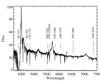
Figure 1: Sloan Digital Sky Survey spectrum of DLA-B/FJ0812+32 (plate 861, fiber 333), with wavelengths in Å along the x-axis, flux ($f_{\lambda}*10^{17}{\rm erg\,s^{-1}\,\,{\rm cm^{-2}}\,\AA^{-1}}$) along the y-axis, and the $1\sigma$ error in gray. This example shows a bit of the Ly$\alpha$ forest between 4200-4450 Å, the damped Ly$\alpha$ profile of log $N_{\rm HI}=21.35$ near 4400 Å ($z_{abs}=2.626$), and QSO Ly$\alpha$  NV, Si IV & OIV, and C IV emissions near 4500, 4600, 5200, 5700 and Å, respectively ($z_{em}=2.701$). Various strong metal absorption lines can be seen scattered redward of the QSO Ly$\alpha$ emission peak, many of them associated with the DLA system (marked; the longer dashes show the key metal-strong transitions Si II 1808 and Zn II 2026). This is a bright QSO ($r=17.46$ mag) and therefore this spectrum has high SNR for SDSS data.

3.1 SDSS Search Algorithm and Visual Inspection

This section describes the codes we developed to identify metal-strong DLA candidates in the SDSS quasar spectra. These algorithms are now available as part of the XIDL package developed by J.X. Prochaska; see http://www.
ucolick.org/$\sim$xavier/IDL/index.html. Our strategy was to identify all significant absorption features redward of the Ly$\alpha$ forest and search for sets of these lines which have a common absorption redshift. The search is complicated by the (possible) presence of other metal lines associated with separate systems along the same sightline as well as telluric lines from our atmosphere.

We set the minimum redshift of this survey to $z_{abs}=1.6$ because the Earth’s ozone (${\rm{O}}_{3}$) layer blocks UV radiation below 3000 Å and, therefore, the Ly$\alpha$ profile cannot be observed at $z_{abs}<1.6$ with ground-based telescopes. Follow-up UV observations are largely unattainable because of the current lack of space-based UV facilities with the requisite wavelength coverage and resolution. SDSS spectra have a starting wavelength at $\approx 3800$Å such that systems with $z_{abs}<2.1$ have their Ly$\alpha$ profile blueward of the SDSS spectra. It is nevertheless worthwhile to extend the search to $z=1.6$ rather than $z=2.1$, because we expect to observe more metal-strong systems at lower redshift given: (1) galaxies enrich in time (Prochaska et al., 2003); and (2) the QSO luminosity function peaks at $z_{em}\sim 2$ providing many additional targets at $z<2.2$. Also, extending the search to $z=1.6$ is worthwhile simply because we’d like to increase our chances of of finding potentially rare metal-strong DLAs. Many of our metal-strong candidates are detected at $z_{abs}<2$ and therefore have no corresponding Ly$\alpha$ profile in the SDSS spectra. Follow-up observations with medium-sized ground-based telescopes will provide the H I measurements necessary for determining metallicities and ionization fractions of the systems.

The first step in our analysis is to process every quasar with the algorithm sdss_qsolin. This routine fits a continuum to each spectrum using a principle component analysis (PCA) developed by S. Burles. It then convolves each spectrum with a Gaussian of FWHM$=$2.5 pixels (chosen to match the width of unresolved metal profiles in SDSS) and records any resulting absorption features that are detected to be $\geq 3.5\sigma$. Finally, the code records the wavelengths of all features separated by more than 4 pixels; multiple features identified with smaller separation are recorded as a single line. We restrict the metal search to the spectral region redward of the QSO Ly$\alpha$ emission to (1) avoid misidentifying Ly$\alpha$ forest lines as metal absorption, and (2) simplify the automated continuum fitting. We estimate that a negligible amount of candidate metal-strong systems are missed by avoiding the Ly$\alpha$ forest in our metal search, largely due to the possibility of lone Mg II systems being retained by the algorithm, as well as the broad $\lambda_{rest}$ range of other typically strong lines used in the search (see Table The Metal-Strong Damped Ly$\alpha$ Systems). Also note that this issue is particularly negligible when considering the MSDLA fraction computed in $\S$ 7.1, due to the availability of Ly$\alpha$ absorption and high $\lambda_{rest}$ transitions (eg. Mg II & Fe II).

The wavelengths of the detected features are then sent to sdss_search (the controlling code for sdss_metals,
sdss_compare and sdss_dla, the latter detailed in Prochaska & Herbert-Fort 2004) where they are matched against 14 redshifted metal transitions (see Table The Metal-Strong Damped Ly$\alpha$ Systems). These 14 transitions were chosen due to their frequent occurrence in high-redshift DLAs; the ions are typically present in large amounts (due to SNe enrichment from massive stars) and/or have large oscillator strengths. We systematically redshift the 14 lines from $z=1.6$ to $z_{em}$ in increments of 0.0001 in $z$. For each corresponding absorption feature in the observed spectrum within the local dispersion $\Delta\lambda$ of the spectrograph (roughly 1 Å pixel^-1 near 4000 Å to 2 Å pixel^-1 near 8000 Å), the algorithm records a match. The matched wavelengths are also restricted to be $>1230\times$(1+$z_{em}$) to avoid misidentifying QSO-associated Ly$\alpha$ absorption as metal absorption, and regions of the spectrum containing severe atmospheric effects (particularly in the red) are avoided. If more than 10 lines were identified redward of 8000 Å, this region is flagged for severe sky effects and is not included in any further analysis. Otherwise, the search terminates at 9200 Å.

At each redshift, we calculate a percentage-based detection to be the ratio of matches to the number of possible matches; $P=n/m$, where $n$ is the number of matched transitions and $m$ is the number of possible matched transitions, specifically those lying in the spectral coverage (excluding the Ly$\alpha$ forest) and not in a masked sky area. We are especially interested in detecting the Si II 1808 transition (after examining many SDSS spectra we have determined that it is an excellent metal-strong indicator; see $\S$ 5 below); therefore, we do not include it as a possible match (the $m$ of our percentage-based detection), but do increment $n$ if this line is detected. We then define candidate absorption systems to be at those redshifts where $P>60\%$ and $n>1$. If two or more of these systems lie within $\Delta z=0.01$ we combine them into one system (to account for wide absorption line systems and the low resolution of SDSS spectra). Finally, the redshift, the percentage of detection and number of line matches, $n$, of each detected metal system are recorded. The latter two are then used to assign each system an overall quality rating in sdss_compare.

The final step was to visually inspect every detected system with a customized tool, sdss_finchk, and visually rate the strengths of the metal absorptions. Each system was subjectively rated as either ‘bizarre’, ‘none’, ‘weak’, ‘medium’, ‘strong’, or ‘very strong’, depending on the
amount and strengths of the lines present in the system. We mostly used the presence of Si II 1808 to judge ‘strong’ and ‘very strong’ systems in SDSS, as Zn II may often be buried in the noise of low-SNR SDSS spectra. If the minimum depth of the Si II 1808 profile $F_{min}/F_{q}\approx 0.9$ where $F_{q}$ is the quasar flux, then the system was rated as ‘strong’. If the normalized intensity was $F_{min}/F_{q}\leq 0.85$ the system was rated ‘very strong’. Note that this is a subjective visual inspection and the minimum depths were chosen based on experience of looking at many SDSS Si II 1808 absorption profiles. Any other metals present were also taken into account, especially if the Zn II 2026 line was covered. Candidates that were found as a result of confusion with severe noise or sky lines were rated ‘bizarre’. For reference, a summary of our subjective metal-rating scale is shown in Table 2.

All 435 ‘strong’ and ‘very strong’ candidate systems from our search in SDSS-DR3 ($z_{abs}\geq 1.6$) are compiled in Table 3. The complete table is available in the electronic (online) version of this paper; we present only a sample here. Table 3 lists SDSS plate, MJD, and fiber, together with RA, Dec, $r$, $z_{em}$, $z_{abs}$, the overall quality rating of each system (18 is the highest with a strong candidate DLA automatically detected by sdss_dla, otherwise 10 if the system lacks Ly$\alpha$ coverage) and our metal rating from visual inspection (4=‘strong’, 5=‘very strong’). Most ($\frac{17}{27}\approx 63\%$) systems in our ESI sample (described below) were taken from the ‘very strong’ category, while the remainder are all classified as ‘strong’. Broad absorption line (BAL) spectra (see Barlow & Junkkarinen, 1994) were avoided if determined to be too severe (via subjective visual inspection), as these are often associated with the QSO itself and can significantly confuse any subsequent absorption analysis. Approximately 3% of the SDSS-DR3 quasar sample were flagged as BALs (PHW05).

3.2 SDSS Search Results

Of the 19,435 SDSS-DR3 QSO sightlines with $z_{QSO}\geq 1.6$, 2,352 systems show metal absorption ranging from ‘weak’ to ‘very strong’ (ie. all but the ’bizarre’ and ’none’ categories). 16,649 sightlines (86% of those searched) were without sufficient features resembling DLA and/or metal absorption to be retained by the algorithm (note that, for example, a single C IV absorption system won’t satisfy our search criteria). From the set of 2,352 candidate metal absorbers (not yet limited to $r<19.5$), we rated 285 (12%) as ‘strong’ (S) and 150 (6%) as ‘very strong’ (VS) systems (see Table 3). Of the 78 systems categorized as ‘strong’ with $z_{abs}\geq 2.2$, 74 (95%) show a corresponding DLA, while 3 of the 4 others have $N_{\rm HI}$ within $1\sigma$ of the DLA threshold. The exception at $z=2.44$ toward J150606.82+041513.1 (SDSS plate and fiber [589,547]) has a measured log${N({\rm HI})}=19.65\pm 0.15$ at $z_{abs}=2.44$ and represents a rare subset of the super-LLS population. Therefore, we report that $<5\%$ of S absorbers in our sample (with observable Ly$\alpha$ profiles in SDSS) are not DLAs. Of the 41 VS systems with $z_{abs}\geq 2.2$, 100% show a corresponding DLA in the SDSS spectra. Even allowing for an evolution in the $N_{\rm HI}$ distribution of metal-strong candidates between redshifts $1.6<z<2.2$, we contend that only a very small fraction of our MSDLA candidates are not truly DLAs. We are therefore confident in having identified a metal-strong DLA population while lacking Ly$\alpha$ coverage on most systems. However, the presence of a larger fraction of lower $N_{\rm HI}$ systems cannot be excluded until $N_{\rm HI}$ values are obtained for all systems in our sample.

Note, however, that we do have one confirmed super-LLS case in our sample – discussed below; also see Péroux et al. (2006) for another possible example of such a system, although note that the $N_{\rm HI}$ value of the Péroux et al. (2006) system was within $0.5\sigma$ of the DLA threshold, and an independent analysis of the same data from Rao et al. (2005) found it to be a bona fide DLA with log${N({\rm HI})}=20.54\pm 0.15$. Other systems with low $N_{\rm HI}$ and high metallicity have also been found at lower redshifts ($z<1$) by Pettini et al. (2000) and Jenkins et al. (2005; note that this system lies at $z\approx 0.08$, ie. far below the range studied in this work).

4 ESI Observations, Data Reduction and Measurements

4.1 ESI Observations and Data Reduction

To test our automated selection method we compiled a list of our strongest candidate metal absorption systems from SDSS and acquired 27 moderate-resolution spectra using ESI on UT December 20th, 2003, and September 10th and 11th, 2004, at the 10m Keck II telescope. The SNRs of our ESI spectra range from $\approx 10-20$ per pixel with a typical value of $\approx 16$. ESI has a pixel size of $\approx 11$ km s^-1 , and a $0.5^{\prime\prime}$ slit covers 3 pixels for a FWHM of $\approx 34$ km s^-1 . The wavelength coverage is roughly 4,000 Å - 10,200 Å. Table 4 presents a log of our observations listing QSO name, SDSS plate, MJD and fiber, QSO emission redshift ($z_{em}$), $r$ magnitude, exposure time, slit width, and observation date.

The data were reduced with the ESIRedux software package (Prochaska et al. 2003a; see http://www2.keck.hawaii
.edu/inst/esi/ESIRedux/). This package converts 2D
echelle spectra into 1D, wavelength-calibrated spectra. The $1\sigma$ array is also calculated during the reduction process. We continuum-fit each QSO separately with custom software, x_continuum, by fitting high-order polynomials to separate pieces of the spectrum containing no significant absorption. The fit pieces are patched together to create a smooth trace of the QSO continuum. We caution the reader that no errors from our continuum-fitting are taken into account. This is a significant source of error when measuring very weak lines and so we report many such cases as upper limits. Note that continuum error will be comparable to the statistical error for $<4\sigma$ detections but negligible otherwise.

4.2 Measurements from ESI data

Ionic column densities are determined using the apparent optical depth method (AODM; Savage & Sembach 1991, also Jenkins 1996), except when determining
$N({\rm{ZnII\ 2026}})$ and $N({\rm{ZnII\ 2062}})$ (discussed below in
$\S$ 4.2.2). Only lines that have been detected at $\geq 3\sigma$ are listed as measurements. We begin a measurement by plotting the continuum-normalized profile in velocity space with an arbitrary zero-velocity centered on the redshift $z_{abs}$ of the system (usually determined from the strongest of all visible transitions). As examples, selected velocity plots from two systems are shown in Figures 2 and 3. Our full ESI velocity plot sample can be retrieved from the electronic edition of the journal. If an absorption line is determined to be saturated (equivalent width $W>600$mÅ,; see Prochaska et al. 2003 and below), ${N({\rm X})}$ may be treated as a lower limit to the true column density. However, note that saturation effects based on $W$ measurements alone may be misleading for systems with wide velocity widths, as is clearly the case with SDSS0016–0012 (integrated velocity width $\approx 1000$ km s^-1 wide). See below for more discussion of saturation effects and its impact on MSDLA classification for Keck ESI data. The ${N({\rm X})}$ values are reported as upper limits if a feature is detected at less than $3\sigma$ statistical significance.

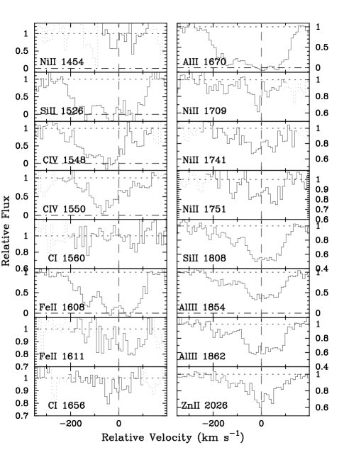
Figure 2: Sample ESI velocity plot 1, with $v=0$ corresponding to the redshift of the absorption system (SDSS0008–0958, $z_{abs}=1.768$). The dashed lines trace the normalized continuum. Line blending is indicated with dotted lines and were not included in the measurements. Note the structure seen in unsaturated lines.

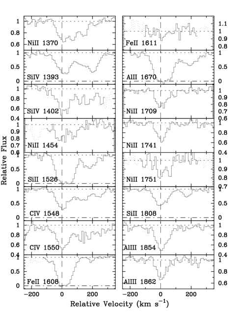
Figure 3: Sample ESI velocity plot, same as Figure 2 but for SDSS0844+5153 at $z=2.77489$.

The electronic edition of the journal also presents tables of ionic column densities for each QAL system in our metal-strong sample. Each table lists ions, rest wavelengths in Å, a flag (0-5) distinguishing primary/non-primary ions and/or limits, $N(\rm{ion})$ as determined from the AODM and $N(\rm{element})_{adopt}$ (determined to be the weighted mean of the primary ion column densities). Any solar values used in the analysis are taken from Grevesse et al. (1996).

4.2.1 Saturation of ESI spectra and the MSDLA definition

Here we emphasize the importance of saturation effects in Keck ESI spectra. We find (in this study and from previous experience with ESI data) that absorption profiles extending below normalized intensities $F_{min}/F_{q}\leq 0.4$ are typically saturated and must be treated as lower limits to the true column densities. In light of this, we treat systems with saturated Zn II or Si II profiles above log${N({\rm Zn^{+}})}\geq 13.0$ or log${N({\rm Si^{+}})}\geq 15.8$ as MSDLAs; however, note that true MSDLAs are defined to have log${N({\rm Zn^{+}})}\geq 13.15$ or log${N({\rm Si^{+}})}\geq 15.95$ and we are simply accounting for ESI saturation effects. Indeed, DLA-B/FJ0812+32 clearly illustrates this effect; ESI data show log${N({\rm Zn^{+}})}\approx 13.04$ while KeckI/HIRES yields log${N({\rm Zn^{+}})}\approx 13.15$ because the lines are not fully resolved in the ESI spectrum. Also, ESI data of ${N({\rm Si^{+}})}$ from DLA-B/FJ0812+32 shows log${N({\rm Si^{+}})}\\ >15.78$ whereas HIRES data yields log${N({\rm Si^{+}})}\approx 15.95$, again due to line saturation. Also note the possibility that some very narrow saturated components of these transitions may not even be resolved by HIRES, in which case the true column densities could be even higher, and so some systems below the ESI-saturation MSDLA threshold might also truly be MSDLAs. Such cases could raise the MSDLA fraction higher than is reported below ($\S$ 7.1).

4.2.2 Mg I and Cr II contributions to Zn II

Pettini et al. (1994) emphasized (for the DLAs) that the Zn II 2026 profile is blended with a weak yet potentially important Mg I 2026 transition. York et al. (2006) have recently shown that in some cases (eg. their Sample 21) that Mg I may dominate the absorption profile at $\lambda_{rest}=2026$Å (as we also find in a few systems), causing concern for any study examining Zn II abundances, particularly for strong systems. Although the Mg I 2026 line has not been well surveyed in the damped Ly$\alpha$ systems (Prochaska & Wolfe, 2002), we suspect that this contribution (in MSDLA candidates) is significantly larger than the average. The likely explanation is that the metal-strong absorbers correspond to higher density regions (sightlines probing nearer the enriched central regions of galaxies) and so one observes a higher fraction of Mg⁰ atoms per Zn⁺ ion.

Because our observations generally include the Mg I 2852 transition, we can estimate the equivalent width of the Mg I 2026 transition (assuming the linear curve of growth, or COG) from the column density measured for Mg I 2852 (with the AODM) and therefore its contribution to the line-profile at $\lambda_{rest}=2026$ Å. In turn, we can measure a more reliable value for ${N({\rm Zn^{+}})}$ from the equivalent width of the remaining Zn II transition at $\lambda_{rest}=2026$ Å (again assuming the linear COG). An inspection of Table 5 shows that the equivalent width of the Mg I 2026 line often contributes $>20\%$ (with a large scatter) of the total equivalent width measured at $\lambda_{rest}=2026$ Å. For those cases where we expect a saturation correction for Mg I 2852, we have incremented the column density by 0.1 dex. This rather small adjustment is due to the fact that the line-profiles are generally not heavily saturated (specifically, follow-up observations with HIRES indicate a 0.1 to 0.2 dex correction is appropriate given the observed peak optical depth of these lines at ESI resolution). We caution that this correction may be misleading for the strongest Mg I systems and that such cases could lead to an overestimate of ${N({\rm Zn^{+}})}$. Higher-resolution data will be useful for examining this effect in particular systems. Furthermore, we have visually inspected every Zn II 2026 profile and find no evidence for severe Mg I 2026 contamination for those DLA where we report a ${N({\rm Zn^{+}})}$ value. Also note that in many cases (see Table 5) the profile of this transition is either noisy (due to low SNR in a particular section of our echelle data), blended with sky and/or profiles from unrelated systems, or simply weak and perhaps at $<3\sigma$ statistical significance if considering continuum-placement errors, and we report ${N({\rm Zn^{+}})}$ as an upper limit.

Similar to the Mg I blending issue is the blending of Cr II and Zn II at $\lambda_{rest}=2062$ Å. This effect was estimated in the same manner as with Mg I (above; yet with both Cr II transitions at $\lambda_{rest}=2056$ and 2066 Å whenever possible) and we calculate an independent value of ${N({\rm Zn^{+}})}$ at $\lambda_{rest}=2062$ Å, whenever possible. We find that Cr II significantly dominates the 2062 profile in most cases. When taken together we find (and list in the tables and use in all plots) the Mg I and Cr II blend-corrected values of ${N({\rm Zn^{+}})}$. Nevertheless, one must always keep in mind the limited resolution of the ESI and that equivalent width measurements may also underestimate ${N({\rm Zn^{+}})}$.

5 SDSS Metal-Strong Indicators

Having identified all potential metal-strong systems in SDSS-DR3, we determine rest equivalent widths $W$ for transitions detected in both the SDSS and ESI spectra. $W$ is the normalized, intensity-weighted width of a line (here in mÅ), and corresponds to the fractional energy absorbed by the transition. This quantity is independent of instrument resolution and is a good predictor of column density for weak lines. Strong lines tend to be saturated; in this regime, $W$ grows with log${N({\rm X})}$ and so a line has roughly the same $W$ as ${N({\rm X})}$ increases. As a result, $W$ is not a reliable column density predictor for strong lines and we must identify the most reliable weak lines as metal-strong indicators in low-resolution spectra.

We have determined that Si II 1808 and Zn II 2026 are usually evident in the metal-strongest absorption systems in SDSS. These two elements are typically only mildly depleted, making them useful indicators of MSDLAs. We measured $W_{r}$ values for Si II 1808 and Zn II 2026 in both the SDSS and ESI spectra for the subset of systems observed with ESI. However, recall that the Zn II 2026 transition is typically blended with Mg I 2026. Table 6 lists the QSO name, SDSS plate and fiber, $z_{em}$, $z_{abs}$, $r$, log$N_{\rm HI}$ if available, log${N({\rm SiII\ 1808})}$, log${N({\rm ZnII\ 2026})}$ (blend-corrected), and $W_{r}(1808)$ and $W_{r}(2026)$ from both SDSS and ESI data. The idea here is to roughly estimated $W_{r}$ values in SDSS data to gauge a system’s metal-strong potential when observed at higher resolution. We assign conservative $\sigma_{W}$ estimates on SDSS data of 50 mÅ. Figure 4 shows a plot of our $W_{r}$ measurements for the absorption profiles at $\lambda=1808$ and 2026Å from SDSS and ESI observations, for systems with secure column density values. The majority of measurements lie within $2\sigma$ of each other, although weaker lines are found to have a systematically higher, false contribution from noise in lower-resolution and lower-SNR SDSS data. Overall, however, we conclude that using $W_{r}(1808)$ and $W_{r}(2026)$ from SDSS is a reliable means of gauging a system’s metal-strong potential in higher resolution spectra.

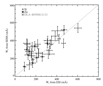
Figure 4: Rest equivalent width values $W_{r}$ from ESI vs. $W_{r}$ from SDSS for both Si II 1808 and Zn II 2026, for all cases with secure column density values. The value for DLA-B/FJ0812+32 is plotted in gray. Note that these values do not account for minor blends, low SNR or saturation effects; weaker $W_{r}$ lines systematically have higher, false contribution from noise in lower-resolution and lower-SNR (SDSS) data.

We now investigate how $W_{r}$ estimates from SDSS correlate with column density values measured from the ESI data. Figures 5 and 6 show $W_{r}$ from SDSS vs. log$N$ from ESI for Si II 1808 and Zn II 2026, respectively (exact $\sigma_{N}$ values can be found in the abundance tables of the electronic version of the paper; roughly 0.07 dex for Si II 1808 and 0.10 dex for Zn II 2026). We expect smaller $W_{r}$ values to be more reliable indicators of $N$ (they are weak, unsaturated lines), and indeed we see a larger scatter in the larger and possibly saturated $W_{r}(\rm{Si\ II\ 1808})$ values. We therefore expect that Zn II 2026, although less often detected in SDSS spectra, is a more reliable indicator of potential MSDLAs than is Si II 1808. Considering Figure 6, we tentatively expect that most SDSS systems with $W_{r}(\rm{Zn\ II\ 2026})>300$ mÅ will be truly metal-strong when measured at higher resolution, supporting a choice to skip the moderate-resolution confirmation observations of such systems. Note that our ESI measurements of Zn II lines near log${N({\rm Zn\ II\ 2026})}\approx 13.0$ are systematically underestimated by 0.1 to 0.2 dex due to line saturation. Si II 1808, however, is detected more often than Zn II 2026 in the SDSS spectra and may be the only indicator for low-resolution, low-SNR data. We therefore propose a similar tentative $W_{r}(\rm{Si\ II\ 1808})$ metal-strong threshold of 450 mÅ, past which we will skip medium-resolution observations (also note here that our ESI measurements of Si II lines near log${N({\rm Si\ II\ 1808})}\approx 15.8$ may be viewed as underestimates due to line saturation). For optically-thin gas, a $W_{r}(\rm{Zn\ II\ 2026})=300$ mÅ profile corresponds to log${N({\rm Zn^{+}})}\approx 13.2$, and a $W_{r}(\rm{Si\ II\ 1808})=450$ mÅ profile corresponds to a log${N({\rm Si\ II\ 1808})}\approx 15.9$. With the overall goal of this project being to discover more systems like DLA-B/FJ0812+32 we are excited to see that many systems far surpass it in ${N({\rm Si^{+}})}$ and ${N({\rm Zn^{+}})}$. These systems may show transitions not yet observed in the young universe and could be used to constrain theories of nucleosynthesis and galaxy evolution, as did DLA-B/FJ0812+32. We will present detailed results of KeckI/HIRES and VLT/
UVES observations of these new systems in upcoming papers.

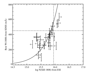
Figure 5: $W_{r}(1808)$ from SDSS vs. log ${N({\rm SiII\ 1808})}$ from ESI. DLA-B/FJ0812+32 is plotted in gray as a lower limit to ${N({\rm Si^{+}})}$. Also plotted in black dashed linestyle are the proposed log${N({\rm Si^{+}})}$ and $W_{r}(1808)$ metal-strong thresholds. Note that ESI values may be underestimated for log ${N({\rm SiII1808})}>15.8$ due to possible saturation. The solid black line traces $W_{r}(\rm{SiII\ 1808})$ vs. ${N({\rm SiII\ 1808})}$ for optically-thin gas.

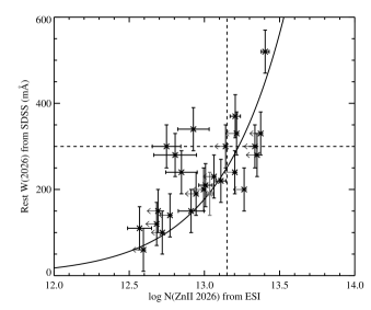
Figure 6: $W_{r}(2026)$ from SDSS vs. log ${N({\rm ZnII\ 2026})}$ from ESI. DLA-B/FJ0812+32 is plotted in gray. Also plotted in black dashed linestyle are the proposed log${N({\rm Zn^{+}})}$ and $W_{r}(2026)$ metal-strong thresholds. Note that ESI values may be underestimated for log ${N({\rm ZnII2026})}>13.0$ due to possible saturation. The solid black line traces $W_{r}(\rm{ZnII\ 2026})$ vs. ${N({\rm ZnII\ 2026})}$ for optically-thin gas.

6 Equivalent Width and SNR Estimates for Detecting Very Weak Lines

To reliably constrain theories on the production of elements like B, O, Sn, Pb and Kr, higher-resolution data is needed. Some of these lines (BII $\lambda$1362, O I $\lambda$1355, SnII $\lambda$1400, Pb II $\lambda$1433, and KrI $\lambda$1235) are still out of reach to modern instruments and with reasonable integration times. Nevertheless, it is interesting to estimate how strong they might be in our sample of metal-strong DLA galaxies for which we have reliable measurements of other elements. These extremely weak lines are presumed to lie buried in our metal-strong ESI data, yet it may be possible to bring them out with lengthy HIRES observations (assuming that they lie in detectable spectral regions). As a brief exercise we predict the SNRs it would take to detect such features at $3\sigma$.

Because we are interested here in detecting weak lines, we will make use of the weak limit of equivalent width,

$$W_{obs}({\rm X})={\pi e^{2}\over m_{e}c^{2}}\lambda_{r}^{2}(1+z)N({\rm X})f\;\;,$$ (1)

where $W_{obs}(\rm X)$ is the observed equivalent width of transition X and ${N({\rm X})}$, $\lambda_{r}$ and $f$ are the column density, rest wavelength, and oscillator strength of the line, respectively. Because we have not yet measured the weak lines, we must first estimate their $N$ values from other reliable line measurements in their corresponding systems. To do this, we assume that the column densities scale with their solar abundances (ie. [X/Y]=0 with X the undetected element and Y a detected reference element) with no corrections. Next, a reliable reference element is chosen. Because Fe is highly refractive, we will choose the mildly depleted element Si (we have the most measurements of Si after Fe). Using

$$\log{[N({\rm X})/N({\rm{X}})_{\sun}]}=\log{[N({\rm Si})/N({\rm{Si}})_{\sun}]}$$ (2)

to scale the abundances to solar values, one can easily solve for ${N({\rm X})}$ and hence $W_{obs}(\rm X)$.

To determine what SNR is needed for a $3\sigma$ detection, it can be shown that

$${\rm{SNR}}=\frac{3}{W_{obs}}\sqrt{{\frac{{\rm V}\lambda_{obs}\Delta\lambda}{c}}}\;\;,$$ (3)

assuming $\sigma_{i}$ (the normalized error of the spectrum) and $\Delta\lambda$ are constant across the V velocity width feature. This is a reasonable assumption for metal lines in the weak limit (and if they are narrow features). Here $\Delta\lambda$ is the HIRES dispersion element in mÅ/pixel at the wavelength of the feature and $c$ is the speed of light.

Figure 7 shows the limiting $W_{obs}$ detection lines vs. SNR (per 2 km s^-1 pixel) for a V = 20 km s^-1 absorption profile detected at $3\sigma$ and plotted for $\lambda_{obs}=4000$ Å (black) and 5000 Å (gray). As an example, we investigate predictions for the observed B II 1362 line in the DLA-B/FJ0812+32 HIRES spectrum from Prochaska, Howk, & Wolfe (2003) (V $\approx 20$ km s^-1 , $\lambda_{obs}=4940$ Å). The dotted line shows $W_{obs}$ of B II in DLA-B/FJ0812+32 as predicted from ESI data assuming [B/Si] = 0 ($W_{obs}>6$ mÅ; a lower limit because log${N({\rm Si^{+}})}>15.78$ in the ESI data). The dashed line is the predicted $W_{obs}$ of B II using the log${N({\rm Si^{+}})}=16.0$ measurement from HIRES as reference. In the HIRES spectrum, we measure the B II $W_{obs}\approx 18$ mÅ for a SNR $\approx 30$ (per 2 km s^-1 pixel). The offset between the observed and predicted $W_{obs}$ values is due to our assumption that the column densities scale with their solar abundances with no corrections. Indeed, in this case the gas-phase B/Si abundance is super-solar and we therefore expect the observed value to be found above the predicted value.

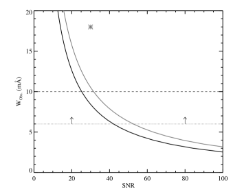
Figure 7: Limiting $3\sigma$-detection lines of $W_{obs}$ vs. SNR (per 2 km s^-1  pixel) for a V = 20 km s^-1  profile observed with HIRES at 4000Å (black) and 5000Å (gray). The dotted line shows $W_{obs}$ of B II 1362 in DLA-B/FJ0812+32 as predicted from ESI data ($W_{obs}>6$ mÅ; a lower limit because the reference element used, Si, is a lower limit in the ESI data, log${N({\rm Si^{+}})}>15.8$). The dashed line is the predicted $W_{obs}$ of B II 1362 using the log${N({\rm Si^{+}})}=16.0$ measurement from HIRES as reference. In the HIRES spectrum, we measure the $W_{obs}\approx 18$ mÅ for a SNR $\approx 30$ (per 2 km s^-1 pixel), marked here as the gray star.

One can then determine how the velocity width V of a line relates to SNR for a fixed $W_{obs}$. Lines near $W_{obs}=10$ mÅ should be trivial to detect at $3\sigma$ with HIRES. Lines below $W_{obs}=5$ mÅ quickly become too difficult to detect (for $W_{obs}=5$ mÅ and V $=$ 4, 10 and 20 km s^-1, SNRs are $\approx$ 25, 40, and 55, respectively) and features near $W_{obs}=1$ mÅ are at the HIRES detection limit for faint quasars (for V $=$ 4 km s^-1, SNR is $>100$; for V $=$ 16 km s^-1, SNR is $>200$).

Therefore, we determine that lines with $W_{obs}\geq 5$ mÅ would be detectable with observations similar to those of DLA-B/FJ0812+32. This implies that many B II 1362 and O I 1355 lines, if in detectable regions of the spectrum, will be observed with future HIRES observations. Many of the predicted Sn, Pb, and Kr equivalent widths are currently out of reach (for example $W_{obs}=2.5$, 1.8 and 4.3 mÅ  respectively, for DLA-B/FJ0812+32 assuming log${N({\rm Si^{+}})}=16.0$), but our SDSS metal-strong sample includes a number of excellent candidates for observations with future instruments.

7 Implications for Damped Ly$\alpha$ Systems

7.1 Metal-Strong DLAs

Given the results from our ESI observations, we may now return to our SDSS MSDLA candidates and estimate the fraction of DLAs that are truly metal-strong. This may help us determine if previous analyses of DLA chemical evolution have suffered from small sample sizes. Our SDSS-DR3 DLA Survey (PHW05) presents $N_{\rm HI}$ measurements of 525 DLAs automatically detected in the SDSS-DR3 QSO sample, which is $\approx 10\times$ larger than the combined QSO sample size of previous samples at $z_{abs}\approx 3$ (Péroux et al., 2003). Noting that the SDSS-DR3 DLA Survey is $>95\%$ complete (and $100\%$ for log $N_{\rm HI}>20.4$, as most metal-strong DLAs tend to be), we may now examine the overall incidence of MSDLAs.

We find $\frac{29}{304}\approx 10\%$ of all DLAs in our SDSS-DR3 DLA Survey (restricted to $r<19.5$) to be candidate S-DLA absorbers, and $\frac{15}{304}\approx 5\%$ of all DLAs in the same sample to be candidate VS-DLA absorbers. Recall that these ratings are largely qualitative and based on the observed absorption depths of Si II 1808 profiles in the SDSS spectra (see $\S$ 3.1). We present these separate categories here to compliment Table 3 and so that the reader may appreciate the differences between the candidate samples. In our ESI sample of 27 QSOs, $\frac{3}{10}=30\%$ of our S candidate absorbers are confirmed as truly metal-strong (i.e. log${N({\rm Zn^{+}})}\geq 13.0$ or log${N({\rm Si^{+}})}\geq 15.8$ in ESI data, accounting for possible saturation effects) while $\frac{9}{17}\approx 53\%$ of our VS candidate absorbers are truly metal-strong. We do not include the upper limits here, even if they lie above the metal-strong threshold. We therefore propose that $(0.30\times 29+0.53\times 15)/304\approx 5\%$ of all DLAs with $z_{abs}\geq 2.2$ observed in QSO sightlines with $r<19.5$ are truly metal strong. This agrees with a similar estimate ($<9\%$) for metal-strong systems as determined from simulations (Ellison 2005 and references therein). Such a result helps explain why previous studies have never clearly identified the MSDLA population, as sample sizes had not been large enough until now.

7.2 Dust Obscuration Bias?

As described in $\S$ 2, we define metal-strong absorbers to have log${N({\rm Zn^{+}})}\geq 13.15$ in accordance with DLA-B/FJ0812+32, also corresponding to the Boissé et al. (1998) obscuration ‘threshold’. However, as it may have been misunderstood in previous works, we emphasize that the Boissé threshold was not intended to be a defining boundary of a ‘forbidden region’ of DLA absorbers (P. Boissé, private communication). The author maintains that a small percentage of DLAs are expected to lie beyond this threshold and should be revealed as optical samples begin probing fainter QSO sightlines. We will argue that at least the region near log${N({\rm Zn^{+}})}=13.15$ is not disfavored by a statistically significant dust bias but that these systems are simply rare.

Figure 8 presents a histogram of log${N({\rm Zn^{+}})}$ from our ESI data. Measurements are plotted as filled gray in the top panel, upper limits as black lines in the bottom panel, and the metal-strong threshold (log${N({\rm Zn^{+}})}=13.15$) as a dashed black line. We emphasize that ESI measurements of Zn lines near log${N({\rm Zn^{+}})}\approx 13.0$ (dashed gray line) are systematically underestimated by 0.1 to 0.2 dex due to line saturation. Therefore, nearly half of the detections in Figure 8 probably match or exceed the metal-strong threshold.

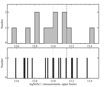
Figure 8: Histogram of log${N({\rm Zn^{+}})}$ from the ESI data (including DLA-B/FJ0812+32, with log${N({\rm ZnII\ 2026})}=13.04\pm 0.02$). Measurements are plotted as filled gray in the top panel, upper limits as black lines in the bottom panel, and the metal-strong threshold (log${N({\rm Zn^{+}})}\approx 13.15$) as a dashed black line. Note that systems with log${N({\rm Zn^{+}})}\approx 13$ (dashed gray line) may be underestimated due to line saturation in ESI spectra.

As mentioned in Boissé et al. (1998) and originally developed in Fall & Pei (1993), significant dust extinction might preferrentially select QSO systems having a low metal content. This follows from the argument that metal-strong systems having a high metal content would likely also have significant dust columns, thereby considerably dimming the background QSO. In magnitude-limited surveys, therefore, one might expect to find the most metal-strong absorbers towards the faint end of the QSO-sightline magnitude distribution. Figure 9 presents log${N({\rm Zn^{+}})}$ vs. $r$ magnitude from our ESI sample. Keeping in mind that systems near log${N({\rm Zn^{+}})}\approx 13.0$ (dashed gray line) are likely underestimated due to saturation, one notices a significant scatter in the $r$ magnitudes consistent with no statistically significant dust bias; a Spearman rank correlation test on the measured values (ie. excluding limits) gives a linear correlation coefficient of 0.49 at $<2\sigma$ statistical significance. However, we emphasize that the true test of this debate lies in observing fainter QSOs. Indeed, our strongest Zn absorber (SDSS1610+4724) does lie among the faintest QSOs in our metal-strong sample; this system in particular is most likely affected by dust obscuration (the results presented in $\S$ 8 find it to have the highest [Mn/Fe] value in the sample, $+0.2\pm 0.1$ dex, as well as high [Zn/Fe] ,$0.7\pm 0.1$ dex, both telltale signatures of dust). And, we also observe a lack of clearly metal-strong systems along the brightest QSO sightlines.

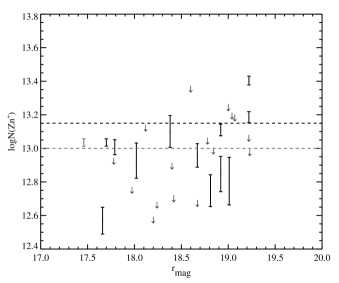
Figure 9: log${N({\rm Zn^{+}})}$ vs. $r$ magnitude from our ESI sample. The metal-strong threshold, log${N({\rm Zn^{+}})}=13.15$, is marked as a dashed black line. DLA-B/FJ0812+32 is marked in gray. Note that systems with log${N({\rm Zn^{+}})}\approx 13$ (dashed gray line) may be underestimated due to line saturation in ESI spectra. A nearly 2 magnitude statistically constant scatter in the magnitudes of metal-strong sightlines is observed; a Spearman rank correlation test on the measured values (excluding limits) gives a linear correlation coefficient of 0.49 at $<2\sigma$ statistical significance. Finding MSDLAs along fainter QSO sightlines (ie. $r>19.5$) will provide a better means to test the effects of dust on this population.

The Boissé et al. (1998) sample contained 37 DLAs, and considering the MSDLA fraction is $\approx 5\%$ it is not surprising that the number of MSDLAs described in that work was zero (also note that the limiting magnitude there was significantly brighter than ours, near $r\approx 18.5$, so systems predicted to be the most strongly affected by dust, the MSDLAs, were even more unlikely to be found in that sample). We contend, however, that a significant dust bias is not evident in either our DLA or MS absorber samples and that MSDLAs are not often discovered at high redshift simply because they are rare. However, we acknowledge the hindrance of not having HI measurements for most of these systems; we have therefore not computed dust-to-gas ratios or ionization fractions for the absorbers in our sample. These values would be critical for a thorough analysis of dust extinction in metal-strong absorbers, and we plan to confront such issues in future papers.

Other works have also been unable to find evidence supporting a significant dust bias on the overall DLA population. Murphy & Liske (2004) presented a spectrophotometric survey of over 70 DLA sightlines from SDSS-DR2 comparing the spectral index distribution of these DLA sightlines with a large control sample and found no evidence for dust-reddening at $z\approx 3$. They placed a limit on the shift of the spectral index $|\Delta\alpha|<0.19$ ($3\sigma$), corresponding to $E(B-V)<0.02$ mag ($3\sigma$) for SMC-like dust, and preliminary SDSS-DR3 results show $\Delta\alpha=-0.063\pm 0.014$ ($1\sigma$ error; $\Delta\alpha$ significant at $\approx 4.5\sigma$), corresponding to $E(B-V)=0.0071\pm 0.0016$ mag and $A_{v}\approx 0.02$ mag for SMC-like dust (Murphy et al. 2006; in prep.). The $E(B-V)$ value is derived by (de-)reddening the DLA QSO spectra according to the SMC-like dust law with different values of $E(B-V)$ in a maximum likelihood analysis. The authors caution, however, that this preliminary result does not yet include any correction for the color selection of the QSOs in SDSS. They expect their $E(B-V)$ result to be somewhat more positive and significant once this is taken into account, with a very preliminary, rough estimate of $\approx<40\%$ effect. This comes from estimates of SDSS completeness at different values of the spectral index in Murphy & Liske (2004). Although the nature of dust in high-redshift galaxies is not well understood, these results indicate a very small reddening of the DLA QSO sightlines and that dust obscuration is therefore not very important for the overall DLA population. The results are inconsistent with earlier studies of Fall, Pei and collaborators, which the authors attribute to the small sample sizes used in previous works.

Furthermore, CORALS I (Ellison et al., 2001) demonstrated that $z>2$ samples of DLAs toward radio-selected quasars show no significant difference from optically-selected samples, and CORALS II (Ellison et al., 2004) indicates only a mild effect at lower redshifts where integrated star formation histories are most significant. Ellison et al. (2005) finds $E(B-V)<0.04$ in CORALS DLAs when comparing optical-to-infrared colors of QSOs with and without intervening absorbers. Finally, Akerman et al. (2005) also found no evidence for increased dust depletions in CORALS DLAs and stated that large scale optical QSO surveys give a fair census of the high-redshift absorber population. However, it should be noted that the CORALS results come from small sample sizes and may not be fully representative of the overall DLA population.

If a significant dust bias did exist one would expect to observe higher $N_{\rm HI}$ values towards fainter QSOs, as these systems would likely have a higher dust content. The SDSS-DR3 DLA Survey (PHW05) presents results that we argue are contradictory to this idea. That work (which includes 525 SDSS DLAs with $z_{abs}>2.2$) shows higher $N_{\rm HI}$ systems towards brighter QSOs. In the paper, PHW05 discuss a variety of systematic effects that may be responsible and conclude with the possibility of gravitational lensing (GL). Indeed, Murphy & Liske (2004) measured an $\approx 2\sigma$ excess of bright and/or deficit of faint SDSS-DR2 QSOs with intervening DLAs and attributed this to GL. That group is currently examining this effect with the increased SDSS-DR3 DLA sample. However, we caution that the effects of dust and GL are quite difficult to disentangle and prefer to refrain from further comment until the interplay between these competing effects is better understood.

In the interest of a balanced discussion of the dust bias on DLAs, we wish to mention recent works supporting the dust bias and touching on strong metal-absorption systems. Notably, Vladilo & Péroux (2005) derived a relation between the extinction of a DLA system and its $N_{\rm HI}$ value, metallicity $Z$, fraction of iron in dust, $f_{\rm{Fe}}(Z)$, and redshift $z_{abs}$. The authors argued that this relation predicts that $\approx 30-50\%$ of all DLAs are missed as a result of their own extinction in magnitude-limited surveys, and show that the empirical thresholds of log${N({\rm Zn^{+}})}\approx 13.2$ and log$N_{\rm HI}\approx 22$ are also quantitative predictions of their model. We claim that such systems are simply rare and therefore not often discovered. Of the handful of MSDLAs we do find in a quasar set of nearly 20,000, we make special note of SDSS1610+4724 with log${N({\rm Zn^{+}})}=13.40\pm 0.03$, clearly above the proposed extinction ‘threshold’ (yet admittedly in a faint QSO sightline, $r=19.22$). The author has proposed that the extinction per metal column density might drop in interstellar environments with extremely high density owing to coalescence of dust grains, and that SDSS1610+4724 could be one of those rare, very interesting cases (G. Vladilo, private communication). If this is not the case, however, SDSS1610+4724 may pose a (perhaps minor) challenge to their model of dust obscuration. Unfortunately, the current lack of Zn measurements precludes an exact estimate of the bias; this makes MSDLAs the critical subclass for gauging the effect.

Also important to these issues is the resemblance between the properties of local dust grains and those in high-redshift clouds; Vladilo et al. (2006) have recently investigated this issue in absorbers out to $z\approx 2$ and find that the mean extinction per atom of iron in the dust is remarkably similar to that found in interstellar clouds of the Milky Way. Also noted in their paper is the previous study by Petitjean et al. (2002) of SDSS0016–0012, a system also found in our sample and with a velocity profile spanning roughly 1,000 km s^-1 . Petitjean et al. (2002) found SDSS0016–0012 to have a high dust content, as well as the highest overall (${\rm{H}}_{2}$) molecular fraction of DLAs at that time, and argued in support of a dust obscuration bias.

We also comment on the large, recent survey of York et al. (2006). This group examined 809 Mg II absorption systems in SDSS and found that the average extinction curves of their sub-samples are similar to the SMC extinction curve with a rising UV extinction below 2200Å. The authors also found that the absorber rest frame color excess, $E(B-V)$, derived from the extinction curves, depends on the absorber properties and ranges from $<0.001$ to 0.085 for various sub-samples. While a notable result, we argue that even systems with $E(B-V)\approx 0.1$ are unlikely to provide a statistically significant dust obscuration bias on the overall DLA population.

Some highly dusty systems have also been discovered at lower redshifts ($z\approx 1$) by Wild & Hewett (2005) and Wild et al. (2006), via strong Ca II absorption. Note that these systems are inferred DLAs from their corresponding Mg II, Mg I and Fe II absorption features. A composite spectrum from the Wild & Hewett (2005) sample yields $E(B-V)\approx 0.06$, while the absorbers from Wild et al. (2006) have on average $E(B-V)>\approx 0.1$.

Finally, to add an overlying word of caution to this entire debate, note the study of Hopkins et al. (2004) who examined SDSS quasars and found that reddening along these lines of sight is dominated by SMC-like dust at the quasar redshifts; that is, not even primarily due to intervening absorbers.

7.3 Effects on the $N_{\rm HI}$-weighted Cosmic Mean Metallicity $<Z(z)>$

Prochaska et al. (2003) demonstrated a statistically significant evolution in the $N_{\rm HI}$-weighted cosmic mean metallicity $<Z(z)>$ from $z_{abs}>2$ DLA absorbers. Here we will investigate how MSDLAs could influence their measurements. The chemical-enrichment (C-E) sample of Prochaska et al. (2003) included 113 DLAs with $z_{abs}\geq 1.6$ and in QSO sightlines with $r<19.5$ mag and 95 DLAs with $z_{abs}\geq 2.2$. When considering the $z_{abs}\geq 1.6$ C-E sample, we find an evolution in $<Z(z)>$ to be $m=-0.27\pm 0.03$, consistent with the Prochaska et al. (2003) value (not cut for $z_{abs}\geq 1.6$). Recall that $\approx 5\%$ of all $z_{abs}\geq 2.2$ DLAs in QSO sightlines with $r<19.5$ mag are expected to be metal-strong. We may then roughly estimate the number of MSDLAs expected in a given DLA sample; we might expect to find roughly five MSDLAs in the $z_{abs}\geq 2.2$ C-E DLA sample. That sample currently contains only one such system, DLA-B/FJ0812+32, the defining MSDLA (recall that log${N({\rm Zn^{+}})}=13.04$ from ESI, whereas HIRES data shows log${N({\rm Zn^{+}})}=13.15$; an example of the above-mentioned ESI saturation issue).

To estimate the effect of a single MSDLA, we add
SDSS1610+4724 (our strongest absorber in Zn, log${N({\rm Zn^{+}})}=13.40\pm 0.03$, and with measured log${N({\rm HI})}=21.15\pm 0.15$; [Zn/H]$=-0.42\pm 0.15$) to the C-E sample. We justify this exercise by the reasoning stated above (ie. expecting $\approx 5$ MSDLAs in this sample), yet we note that adding many more of these systems without also including their corresponding non-MSDLAs would bias the C-E sample to an unjustifiable extent. Figure 10 illustrates that adding this one MSDLA raises $<Z>$ in the $z\approx 2.6$ bin by +0.12 dex, ie. $\approx 2\sigma$. Including this system does not significantly change $m$, however, just a slight increase in the scatter: now $m=-0.27\pm 0.04$ dex.

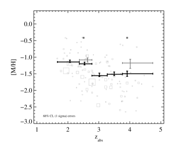
Figure 10: $N_{\rm HI}$-weighted cosmic mean metallicity $<Z(z)>$. DLAs are shown as squares scaled to the $N_{\rm HI}$ of the system (open are from the CE sample, filled are the added SDSS1610+4724 MSDLA). $<Z(z)>$ is plotted for 5 bins with $1\sigma$ uncertainties given by bootstrap analysis. The dark gray errors for the $z_{abs}\approx 2.6$ & 4 bins are the new $<Z>$ values in each bin (offset by 0.1 in $z$ for presentation) after one MSDLA, SDSS1610+4724, is added.

Instead, how might including this same metal-strong absorber at a higher redshift affect $<Z(z)>$ and its evolution? Adding SDSS1610+4724 to the $z\approx 4$ bin of the C-E sample raises $<Z>$ from -1.50 to -1.18 (ie. a +0.32 dex or $\approx 2\sigma$ increase, yet note that such an object being found there is highly unlikely given the current size and statistics of the $z\approx 4$ bin). Nevertheless, the linear $<Z(z)>$ evolution slope also remains nearly identical in this case, $m=-0.26\pm 0.04$, driven by the data with smaller errors. We therefore suggest that MSDLAs could have a modest impact on the $<Z>$ of a single bin yet little impact on the overall DLA $<Z(z)>$ evolution. However, in the unlikely event that one MSDLA was found in each bin under similar statistics, the effect on the linear $<Z(z)>$ evolution slope could be larger.

8 Abundance Analysis from the ESI Sample

We now examine certain abundance ratios from our ESI data and comment on the dust depletion vs. SNe enrichment ‘debate’. Although HIRES data is superior, ESI can still be used to examine global abundance trends.

Before we begin, we must mention here that one system, SDSS0927+5621 ($z_{abs}=1.78$), has a confirmed log$N_{\rm HI}=19.00^{+0.10}_{-0.25}$ (Prochaska et al. 2006, submitted). This system was selected by its metal-strong signature, and metal-strong systems usually are in the $N_{\rm HI}$ range of DLAs. Why is this object both H I-poor and metal-strong? Prochaska et al. (2006, submitted) use HIRES data and find that SDSS0927+5621 is highly ionized, with an ionization factor $x\approx 0.9$ (based on inferences made from the observed $N_{\rm HI}$ and ${\rm{Al}}^{++}$ values). In this case, the QAL system is too far from the QSO to be ionized by it ($z_{em}=2.28$). The extragalactic UV background (EUVB; from QSOs and/or galaxies not in the sightline) is surely a part of the responsible ionizing radiation, but the dominant component likely comes from young, massive stars within the host galaxy. If massive stars are present, one might expect strong-metal absorption (observed), assuming some previous enrichment and energetic feedback processes. Indeed, the authors find SDSS0927+5621 to have wide, complex velocity profiles and propose that such kinematic structure is indicative of feedback processes correlated with star formation. The authors also (tentatively) find SDSS0927+5621 to have the highest gas metallicity of any astrophysical environment and total metal surface density exceeding nearly every known DLA. This system clearly falls into a separate category of QAL systems, the (super-solar) super-LLS, and so we remove it from the following abundance analysis. We caution the reader that the possibility of other assumed DLAs (with $z_{abs}<2.2$) falling into this ‘ionized’ category remains. However, recall that only $\approx 1\%$ of our candidate MS SDSS sample with $z_{abs}\geq 2.2$ was below the DLA threshold. We await $N_{\rm HI}$ measurements from upcoming observations to further comment on this issue.

We also require the systems to have Fe measurements due to the important role of Fe in abundance ratios; therefore, SDSS0316+0040 and SDSS1235+0017 are also excluded from the following analysis. Also note that the relative abundances to be plotted will not involve $N_{\rm HI}$. We have assumed a conservative lower limit of $0.10$ dex error ($1\sigma$) for all measurements and emphasize that such large errors are the most significant hindrance to doing abundance-ratio analysis with this moderate-resolution data.

Figure 11 shows a plot of [Ti/Fe] vs. [Si/Fe] . It is evident here that all the systems in our sample show enhanced Si/Fe ratios. This can be interpreted as either Type II SNe enrichment or depletion of Fe onto dust, or both. Also note that at low [Si/Fe] the [Ti/Fe] values are enhanced. Although Ti behaves like a refractory iron-peak element, in Galactic stars it shows a similar trend as the $\alpha$ elements and is thus generally accepted as an $\alpha$ element; therefore, because both Ti and Fe are refractory and because Ti is more heavily depleted than Fe (Savage & Sembach, 1996), an overabundance of [Ti/Fe] at super-solar [Si/Fe] implies nucleosynthetic $\alpha$-enrichment (Dessauges-Zavadsky, D’Odorico, & Prochaska, 2002). An underabundance of [Ti/Fe], however, may be attributed to depletion of gas onto dust, and we present a few of these candidates here as well. Overall, this plot may suggest Type II SNe enrichment in many of the MS systems presented here.

Figure 11: [Ti/Fe] vs. [Si/Fe] from our ESI sample. The enhancement of Ti/Fe suggests the gas is predominantly enriched by Type II SNe.

Figure 12 shows a plot of [Mn/Fe] vs. [Si/Fe]. The [Mn/Fe] ratios are mostly sub-solar, and agree with previous measured values attributed to nucleosynthetic enrichment (Lu et al., 1996; Ledoux et al., 1998) including from Type Ia SNe (Dessauges-Zavadsky, D’Odorico, & Prochaska, 2002). We expect these observations to support metallicity-dependent Mn yields from both Type Ia and Type II SNe (McWilliam, Rich, & Smecker-Hane 2003), but require log$N_{\rm HI}$ measurements to be certain. In a future paper, we will investigate the differences in Mn yields from Type Ia- and Type II SNe-dominated systems; recent models indicate that particular distinction may soon be discovered at high [Mn/Fe] values. We also aim to address the range of dust-depletion levels in the MSDLAs. Here we present a new super-solar [Mn/Fe] value and another just shy due to the error; these systems present strong evidence for substantial dust depletion.

Figure 12: [Mn/Fe] vs. [Si/Fe] from our ESI sample. Systems with [Mn/Fe] $>0$ and [Si/Fe] $>+0.3$ must be strongly affected by depletion of gas onto dust.

Figure 13 shows [Si/Zn] vs. [Zn/Fe] for systems in our sample with both Si and Zn measurements. One would expect systems displaying subsolar [Si/Zn] values to be more affected by dust depletion than by nucleosynthetic effects because Si is more refractory than Zn. What is observed suggests that some MS systems may indeed contain high amounts of dust (points at high [Zn/Fe] and low [Si/Zn]). Also supporting this idea is Figure 14, where we plot [Si/Ti] vs. [Zn/Fe]. Because Ti is the most refractive, Si/Ti enhancements at super-solar Zn/Fe are likely due to the depletion of Ti and Fe onto dust grains. Prochaska & Wolfe (2002) state that a correlation between these ratios is strong evidence for dust depletion, and although there is a large scatter the limits suggest a weak overall correlation. While some MSDLAs likely contain a large amount of dust and may eventually be observed to have their own dust-obscuration bias (MSDLA samples toward fainter QSOs will best address this issue), we maintain that the overall DLA population is not significantly affected by a dust bias (see previous sections).

Figure 13: [Si/Zn] vs. [Zn/Fe] from our ESI sample, for all systems with measured values of each element. Systems with low [Si/Zn] and high [Zn/Fe] are the strongest affected by depletion effects.

Figure 14: [Si/Ti] vs. [Zn/Fe] from our ESI sample. This plot supports depletion of gas onto dust grains.

9 Summary and Conclusions

To confirm that our automated technique works well, we summarize our metal-strong detections as follows. Our algorithms searched 19,429 SDSS-DR3 QSO sightlines with $z_{QSO}\geq 1.6$ and found 435 visually-confirmed candidate metal-strong absorbers. Of these metal-strong candidate systems with Ly$\alpha$ wavelength coverage available in the SDSS, we find $<5\%$ (and likely near $\approx 1\%$) are without corresponding DLAs, ie. systems belonging to the super-LLS population.

Our metal-searching technique is most sensitive to systems with large $W$ metal profiles, but recall that a large $W$ is not a reliable predictor of $N$ for a saturated transition. Therefore, we focused on weak lines as metal-strong indicators. We plan to use these MS indicators to determine which systems may be directly observed at high resolution without first obtaining medium-resolution confirmation spectra. We argued that $W_{r}(\rm ZnII\ 2026)$ is the best indicator of metal-strong QAL systems and have compared our sample to the SDSS-DR2 spectrum of the metal-strong DLA-B/FJ0812+32 DLA. We also claimed that $W_{r}(\rm SiII\ 1808)$ is not as reliable an indicator as Zn II 2026 but that it can still be useful for faint QSO sightlines.

All of our ESI (27 metal-strong systems with $r<19.5$ mag) sample had the highest score possible from our SDSS-searching algorithms. Our ESI sample is a collection of 10 and 17 subjectively-rated S and VS systems in the SDSS, respectively. Finally, we have measured (with ESI) 11 systems with ${N({\rm Si^{+}})}$ values near or greater than DLA-B/FJ0812+32 (as measured from ESI data) and 5 with ${N({\rm Zn^{+}})}$ greater than or equal to the Zn detection from DLA-B/FJ0812+32 (in the ESI data – recall the importance of saturation effects in MSDLA classification; the HIRES spectrum of DLA-B/FJ0812+32 yields log${N({\rm Zn^{+}})}\\ \approx 13.15$). Therefore, $\approx 40\%$ of the systems in our ESI sample yielded ${N({\rm Si^{+}})}$ or ${N({\rm Zn^{+}})}$ measurements consistent with or higher than DLA-B/FJ0812+32. PHW05 demonstrated that our automated SDSS DLA-finding technique also works well, and we will search future SDSS Data Releases for MSDLAs and publish updated metal-strong candidate lists periodically.

We estimated the feasibility of detecting certain weak transitions at $3\sigma$, predicting what SNRs we would need to reach with HIRES-grade instruments. We find that lines with $W_{obs}\geq 5$ mÅ would be detectable with observations similar to DLA-B/FJ0812+32, and therefore that a handful of B II 1362 and O I 1335 lines may soon be observed in our metal-strong ESI sample. As the collecting power of modern and future telescopes continues to increase (and with it SNRs), we will begin detecting Sn, Pb, and Kr lines in these high-redshift systems. We are currently testing our predictions with KeckI/HIRES and VLT/UVES observations.

Taking our SDSS and ESI results together, we predict that $\approx 5\%$ of all $z_{abs}\geq 2.2$ DLAs in QSO sightlines with $r<19.5$ are truly metal-strong. This result is of particular importance when considering previous results from DLA studies with small sample sizes, especially those proposing a significant dust-obscuration bias on the overall DLA population. Along separate lines of research and with additional results from our SDSS-DR3 DLA Survey, we find no evidence in support of a statistically significant dust-obscuration bias for the overall DLA population. We await a larger, deeper metal-strong DLA sample, complete with UV Ly$\alpha$ measurements to further comment on this issue and its relevance to the MSDLA population.

We then investigated how a single MSDLA might affect the $N_{\rm HI}$-weighted cosmic mean metallicity $<Z(z)>$ as determined from previous DLA studies. We find that adding our strongest Zn absorber (SDSS1610+4724) to the current C-E sample raises $<Z>$ near $z\approx 2.6$ by +0.12 dex ($\approx 2\sigma$). When the same MSDLA is instead added at higher redshift (albeit a more extreme and perhaps currently unrealistic proposition), we find a +0.32 dex increase ($\approx 2\sigma$) in the $z\approx 4$ bin. The overall linear slope of the $<Z(z)>$ evolution remains essentially unchanged in both cases. We therefore contend that MSDLAs may be significant when considering $<Z>$ in a particular bin, yet given the current statistics are not a strong influence on the evolution of $<Z(z)>$ from the overall DLA population.

Although the conservative errors assumed for the relative abundances from our Keck ESI (medium-resolution) data are large, and we lack many Ly$\alpha$ measurements for computing ionization fractions and dust-to-gas ratios, we concluded with a brief discussion of abundance ratios from our ESI sample and find evidence for significant dust depletion in a handful of systems underlying largely Type II SNe enrichment.

10 Acknowledgements

We thank the SDSS team for their incredible survey and the Keck staff for their assistance and hospitality. We acknowledge the privilege of observing from the summit of Mauna Kea as it has long been considered a sacred site within the indigenous Hawaiian community. We thank S. Burles for providing the SDSS continuum-fitting PCA software. Thanks to P. Boissé, G. Vladilo, D. York, J. Bergeron, and N. Prantzos for helpful comments and suggestions, and to M. Murphy for kindly providing and discussing his SDSS-DR3 DLA-reddening results prior to publication. We also thank the referee for helpful suggestions. SHF especially thanks the UCSC Department of Physics for the generous Undergraduate Thesis Award that helped make his December 2003 travel to Keck possible. JXP and SHF were partially supported by NSF grant AST-0307408 and its REU sub-contract. JXP and AMW are partially supported by NSF grant AST-0307824.

Table 1: Atomic Data

Transition	$\lambda$ (Å)	$f$	Ref.
H I-A 1215	1215.6701	0.4164	1
Kr I 1235	1235.8380	0.1871	1
Si II 1260a	1260.4221	1.007	1
O I 1302a	1302.1685	0.04887	1
Si II 1304a	1304.3702	0.094	2
Ni II 1317	1317.2170	0.058	14
C II 1334a	1334.5323	0.1278	1
C II* 1335	1335.7077	0.1149	1
O I 1355	1355.5977	1.25E-6	1
B II 1362	1362.4610	0.987	1
Ni II 1370	1370.1310	0.0769	3
Si IV 1393	1393.7550	0.528	1
Sn II 1400	1400.4000	1.0274	12
Si IV 1402	1402.7700	0.262	1
Pb II 1433	1433.9056	0.87	1
Ni II 1454	1454.8420	0.0323	4
Ni II 1467	1467.2590	6.3E-3	4
Ni II 1467	1467.7560	9.9E-3	4
Si II 1526a	1526.7066	0.127	5
C IV 1548	1548.1950	0.1908	1
C IV 1550	1550.7700	0.09522	1
C I 1560	1560.3092	0.08041	1
Fe II 1608a	1608.4511	0.058	6
Fe II 1611	1611.2005	1.36E-3	7
C I 1656	1656.9283	0.1405	1
Al II 1670a	1670.7874	1.88	1
Ni II 1703	1703.4050	0.006	4
Ni II 1709	1709.6000	0.0324	4
Ni II 1741	1741.5490	0.0427	4
Ni II 1751	1751.9100	0.0277	4
Si II 1808a	1808.0126	2.186E-3	8
Mg I 1827	1827.9351	2.420E-2	17
Si I 1845	1845.5200	0.229	1
Al III 1854	1854.7164	0.539	1
Al III 1862	1862.7895	0.268	1
Fe II 1901	1901.7730	1.009E-4	1
Ti II 1910	1910.7800	0.2020	17
Zn II 2026	2026.1360	0.489	9
Cr II 2026	2026.2690	4.71E-3	10
Mg I 2026	2026.4768	0.1120	1
Cr II 2056	2056.2539	0.105	9
Cr II 2062	2062.2340	0.078	9
Zn II 2062	2062.6640	0.256	9
Cr II 2066	2066.1610	0.0515	9
Fe II 2249	2249.8768	1.821E-3	11
Fe II 2260	2260.7805	2.44E-3	11
C II] 2325	2325.4029	4.780E-8	17
C II]* 2326	2326.1126	5.520E-8	17
C II]* 2328	2328.8374	2.720E-8	17
Si II] 2335	2335.1230	4.250E-6	17
Fe II 2344a	2344.2140	0.114	12
Fe II 2374	2374.4612	0.0313	12
Fe II 2382a	2382.7650	0.32	12
Mn II 2576	2576.8770	0.3508	1
Fe II 2586a	2586.6500	0.0691	12
Mn II 2594	2594.4990	0.271	1
Fe II 2600a	2600.1729	0.239	12
Mn II 2606	2606.4620	0.1927	1
Mg II 2796a	2796.3520	0.6123	13
Mg II 2803a	2803.5310	0.3054	13
Mg I 2852	2852.9642	1.81	1
Ti II 3073	3073.8770	0.1091	1
Ti II 3230	3230.1310	0.0687	15
Ti II 3242	3242.9290	0.232	16
Ti II 3384	3384.7400	0.358	17

References. — 1: Morton (1991); 2: Tripp et al. (1996); 3: Fedchak, & Lawler (1999); 4: Fedchak, Wiese, & Lawler (2000); 5: Schectman et al. (1998); 6: Bergeson et al. (1996); 7: Raassen & Uylings (1998); 8: Bergeson & Lawler (1993); 9: Bergeson & Lawler (1993b); 10: Verner et al. (1994); 11: Bergeson, Mullman, & Lawler (1994); 12: Morton (2001); 13: Verner (1996); 14: Dessauges-Zavadsky et al. (2006); 15: Bizzarri et al. (1993); 16: Pickering, Thorne, & Perez (2002); 17: Morton (2003)

Table 2: Summary of Subjective Metal Ratings of SDSS Candidates

Metals	Label	Rating	Description
Bizarre	B	0	Noise, sky, or unclear detection
None	N	1	No metals observed
Weak	W	2	Usually weak Al II 1670 and/or few other strong metals
Medium	M	3	Usually strong Al II 1670 or Fe II, Mg II but no significant Si II 1808
Strong	S	4	Strong Si II 1808 ($F_{min}/F_{q}\approx 0.90$), perhaps weak Zn II 2026
Very Strong	VS	5	Very strong Si II 1808 ($F_{min}/F_{q}\leq 0.85$) and likely Zn II 2026

Table 3: Metal-Strong Candidates from SDSS-DR3

SDSS plate	MJD	SDSS fiber	RA	Dec	$r$	$z_{em}$	$z_{abs}$	Qualitya	Metalsb
			(J2000)	(J2000)	(mag)
651	52139	494	00:08:15.33	$-09:58:54.0$	18.38	1.951	1.768	10	5
388	51792	607	00:10:17.80	$+01:04:50.7$	18.84	1.817	1.687	10	5
389	51793	332	00:10:25.93	$+00:54:47.6$	19.09	2.847	2.154	9	5
752	52247	194	00:13:41.74	$+14:35:31.3$	19.39	1.933	1.922	10	4
389	51793	497	00:15:49.08	$+00:17:31.9$	19.64	3.066	2.338	7	5
389	51793	178	00:16:02.40	$-00:12:24.9$	18.03	2.087	1.973	10	5
753	52227	430	00:20:28.97	$+15:34:35.9$	18.79	1.764	1.652	10	5
753	52227	550	00:26:15.58	$+15:27:13.5$	19.85	2.914	1.954	9	4
418	51813	452	00:37:49.19	$+15:52:08.4$	20.03	4.072	3.816	17	5
655	52160	51	00:42:05.22	$-10:39:57.5$	19.17	2.490	2.283	10	5
656	52147	269	00:42:19.74	$-10:20:09.4$	18.66	3.881	2.753	14	4
655	52160	635	00:43:49.53	$-09:37:44.0$	18.49	2.130	1.764	10	5
393	51793	495	00:44:39.32	$+00:18:22.7$	18.20	1.866	1.725	10	4
393	51793	62	00:47:15.88	$-00:36:44.0$	18.73	2.198	2.029	10	5
395	51783	121	00:57:09.50	$-00:54:50.9$	18.86	1.885	1.791	10	4
420	51869	12	00:57:57.32	$+14:19:00.0$	19.38	2.154	1.782	9	5
395	51783	445	00:58:14.31	$+01:15:30.3$	17.69	2.495	2.011	10	5
658	52143	490	00:59:45.10	$-09:51:55.1$	20.61	3.036	2.979	8	5
396	51813	535	01:06:48.02	$+00:46:27.9$	18.59	1.877	1.774	10	5

Note. — The complete version of this table is in the electronic edition of the paper. The printed edition contains only a sample.

Table 4: Keck ESI Observations

RA	Dec.		SDSS		$z_{em}$	$r$	Metala	Exp.	Slit width	Obs. date
(2000)	(2000)	Plate	MJD	Fiber		(Mag.)	Rating	(s)	′′	(UT)
00:08:15.33	-09:58:54.3	651	52141	494	1.95	18.38	5	900	0.75	Dec. 20, 2003
00:16:02.40	-00:12:25.0	389	51795	178	2.09	18.02	5	600	0.50	Sept. 10, 2004
00:20:28.96	+15:34:35.8	753	52233	430	1.76	18.78	5	1800	0.50	Sept. 10, 2004
00:44:39.32	+00:18:22.8	393	51794	495	1.87	18.20	4	600	0.75	Dec. 20, 2003
00:58:14.31	+01:15:30.2	395	51783	445	2.49	17.66	5	900	0.50	Dec. 20, 2003
01:20:20.37	+13:24:33.5	424	51893	286	2.57	19.23	5	900	0.75	Dec. 20, 2003
02:25:54.85	+00:54:51.9	406	51869	572	2.97	18.92	4	1800	0.50	Dec. 20, 2003
03:16:09.83	+00:40:43.1	413	51929	387	2.92	18.67	4	1200	0.50	Dec. 20, 2003
08:40:32.96	+49:42:52.9	445	51873	043	2.08	19.00	5	1800	0.75	Dec. 20, 2003
08:44:07.29	+51:53:11.2	447	51877	272	3.20	19.22	5	1800	0.75	Dec. 20, 2003
09:12:47.59	-00:47:17.3	472	51955	210	2.86	18.67	5	900	0.50	Dec. 20, 2003
09:27:05.90	+56:21:14.1	451	51908	071	2.28	18.24	5	900	0.75	Dec. 20, 2003
10:42:52.32	+01:17:36.5	506	52022	137	2.44	18.42	5	600	0.50	Dec. 20, 2003
10:49:15.43	-01:10:38.1	275	51910	006	2.12	17.78	5	600	0.50	Dec. 20, 2003
11:51:22.14	+02:04:26.3	515	52051	223	2.40	18.60	4	600	0.50	Dec. 20, 2003
12:35:59.29	+00:17:16.4	290	51941	463	2.26	18.84	4	600	0.50	Dec. 20, 2003
12:49:24.86	-02:33:39.7	336	51999	073	2.12	17.79	5	900	0.50	Dec. 20, 2003
14:35:12.94	+04:20:36.9	585	52027	628	1.95	19.04	5	600	0.50	Dec. 20, 2003
16:10:09.42	+47:24:44.4	813	52354	621	3.22	18.75	5	1800	0.50	Sept. 10, 2004
16:17:17.83	+00:28:27.2	346	51693	488	1.94	19.07	4	850	0.50	Sept. 10, 2004
16:58:16.47	+34:28:09.8	972	52435	480	1.70	18.40	4	1200	0.50	Sept. 11, 2004
17:09:09.28	+32:58:03.4	973	52426	629	1.89	19.22	5	1800	0.50	Sept. 11, 2004
20:44:31.12	-05:42:39.7	634	52164	634	1.90	18.67	4	1200	0.50	Sept. 10, 2004
20:59:22.42	-05:28:42.7	636	52176	610	2.54	19.12	5	1200	0.50	Sept. 11, 2004
21:00:25.03	-06:41:45.9	637	52174	370	3.14	18.19	5	1200	0.50	Sept. 10, 2004
22:22:56.11	-09:46:36.2	720	52206	203	2.93	17.97	4	600	0.50	Sept. 10, 2004
22:44:52.22	+14:29:15.1	740	52263	390	1.96	18.92	4	1800	0.50	Sept. 11, 2004

Table 5: Zn Analysis

QSO	$W_{2026}$	$W_{2852}$	$W({\rm Mg})^{a}$	$\log{N({\rm Zn^{+}})}_{2026}$	$W_{2062}$	$W({\rm Cr})^{b}$	$\log{N({\rm Zn^{+}})}_{2062}$	$\log{N({\rm Zn^{+}})}$
	(mÅ)	(mÅ)	(mÅ)		(mÅ)	(mÅ)
FJ0812+32	$173\pm 9$	$...$	$...$	$12.99\pm 0.02$	$72\pm 6$	$69$	$11.46\pm 1.12$	$12.84\pm 0.03$
SDSS0008-0958	$383\pm 20$	$934\pm 27$	$37$	$<13.34$	$280\pm 22$	$159$	$13.10\pm 0.09$	$13.10\pm 0.09$
SDSS0016-0012	$190\pm 36$	$997\pm 25$	$39$	$12.93\pm 0.10$	$8\pm 34$	$...$	$<13.02$	$12.93\pm 0.10$
SDSS0020+1534	$170\pm 36$	$843\pm 35$	$37$	$<13.06$	$...$	$88$	$...$	$<13.06$
SDSS0044+0018	$50\pm 23$	$597\pm 28$	$21$	$<12.59$	$...$	$...$	$...$	$<12.59$
SDSS0058+0115	$90\pm 12$	$675\pm 22$	$24$	$12.57\pm 0.08$	$93\pm 16$	$101$	$<12.90$	$12.57\pm 0.08$
SDSS0120+1324	$65\pm 59$	$616\pm 61$	$24$	$<13.00$	$58\pm 55$	$...$	$<13.23$	$<13.00$
SDSS0225+0054	$125\pm 30$	$...$	$...$	$12.85\pm 0.10$	$...$	$178$	$...$	$12.85\pm 0.10$
SDSS0316+0040	$48\pm 29$	$691\pm 40$	$32$	$<12.69$	$1\pm 30$	$...$	$<12.97$	$<12.69$
SDSS0840+4942	$224\pm 74$	$1091\pm 70$	$46$	$<13.26$	$88\pm 59$	$...$	$<13.26$	$<13.26$
SDSS0844+5153	$...$	$...$	$...$	$...$	$187\pm 22$	$184$	$<13.08$	$<13.08$
SDSS0912-0047	$168\pm 27$	$543\pm 48$	$<23$	$12.91\pm 0.09$	$130\pm 34$	$...$	$13.13\pm 0.11$	$12.96\pm 0.07$
SDSS0927+5621	$94\pm 28$	$674\pm 47$	$25$	$<12.68$	$138\pm 29$	$78$	$<13.18$	$<12.68$
SDSS1042+0117	$72\pm 31$	$716\pm 101$	$34$	$<12.72$	$83\pm 28$	$88$	$<13.13$	$<12.72$
SDSS1049-0110	$132\pm 52$	$754\pm 28$	$28$	$<12.94$	$118\pm 37$	$128$	$<13.35$	$<12.94$
SDSS1151+0204	$375\pm 56$	$1606\pm 57$	$66$	$<13.37$	$333\pm 49$	$161$	$<13.41$	$<13.37$
SDSS1235+0017	$...$	$188\pm 66$	$<7$	$...$	$46\pm 33$	$...$	$<13.01$	$<13.01$
SDSS1249-0233	$208\pm 19$	$695\pm 24$	$28$	$13.01\pm 0.04$	$279\pm 19$	$238$	$<12.97$	$13.01\pm 0.04$
SDSS1435+0420	$286\pm 97$	$948\pm 51$	$41$	$<13.21$	$272\pm 57$	$155$	$<13.48$	$<13.21$
SDSS1610+4724	$470\pm 27$	$361\pm 143$	$19$	$13.40\pm 0.03$	$...$	$218$	$...$	$13.40\pm 0.03$
SDSS1617+0028	$269\pm 36$	$1332\pm 41$	$58$	$<13.20$	$169\pm 51$	$124$	$<13.42$	$<13.20$
SDSS1658+3428	$378\pm 35$	$1252\pm 25$	$50$	$<13.35$	$50\pm 26$	$...$	$<12.92$	$<12.92$
SDSS1709+3258	$309\pm 22$	$598\pm 30$	$24$	$13.21\pm 0.03$	$324\pm 24$	$215$	$13.05\pm 0.12$	$13.19\pm 0.03$
SDSS2044-0542	$113\pm 22$	$333\pm 29$	$13$	$12.75\pm 0.09$	$114\pm 24$	$104$	$<13.11$	$12.75\pm 0.09$
SDSS2059-0529	$138\pm 37$	$600\pm 60$	$25$	$12.81\pm 0.14$	$60\pm 35$	$104$	$<13.04$	$12.81\pm 0.14$
SDSS2100-0641	$213\pm 16$	$...$	$...$	$<13.14$	$...$	$145$	$...$	$<13.14$
SDSS2222-0946	$103\pm 17$	$787\pm 63$	$33$	$<12.77$	$...$	$...$	$...$	$<12.77$
SDSS2244+1429	$261\pm 18$	$759\pm 32$	$32$	$13.11\pm 0.03$	$114\pm 22$	$78$	$<13.07$	$13.11\pm 0.03$

Note. — This analysis assumes the linear curve-of-growth for all equivalent width calculations. We may be underestimating the Zn⁺ column density of those systems with equivalent width $>300$ mÅ. Entries with ‘…’ are cases of upper limits to the value (i.e. non-detections).

Table 6: Si II 1808 and Zn II 2026 as Metal-Strong Indicators

QSO name	SDSS	$z_{em}$	$z_{abs}$	$r$	log$N_{\rm HI}$	log${N({\rm SiII\ 1808})}$	$W_{\rm S}(\rm 1808)$	$W_{\rm E}(\rm 1808)$	log${N({\rm ZnII\ 2026})}$	$W_{\rm S}(\rm 2026)$	$W_{\rm E}(\rm 2026)$
FJ0812+32	861-333	2.70	2.626	17.46	21.35*	$>15.78$	$250\pm 50$	$285\pm 8$	$13.04\pm 0.02$	$190\pm 50$	$173\pm 9$
SDSS0008-0958	651-494	1.95	1.768	18.38	…	$16.08\pm 0.03$	$540\pm 50$	$603\pm 33$	$<13.34$	$300\pm 50$	$383\pm 20$
SDSS0016-0012	389-178	2.09	1.970	18.02	20.83**	$15.48\pm 0.11$	$330\pm 50$	$165\pm 46$	$12.93\pm 0.10$	$340\pm 50$	$190\pm 36$
SDSS0020+1534	753-430	1.76	1.652	18.78	…	$15.35\pm 0.09$	$360\pm 50$	$119\pm 26$	$<13.06$	$230\pm 50$	$170\pm 36$
SDSS0044+0018	393-495	1.87	1.725	18.20	…	$<15.51$	$100\pm 50$	$183\pm 31$	$<12.59$	$60\pm 50$	$50\pm 23$
SDSS0058+0115	395-445	2.49	2.011	17.66	…	$<15.82$	$370\pm 50$	$361\pm 25$	$12.57\pm 0.08$	$110\pm 50$	$90\pm 12$
SDSS0120+1324	424-286	2.57	2.000	19.23	…	$<16.04$	$250\pm 50$	$354\pm 68$	$<13.00$	$200\pm 50$	$65\pm 59$
SDSS0225+0054	406-572	2.97	2.714	18.92	21.00***	$15.61\pm 0.07$	$260\pm 50$	$227\pm 35$	$12.85\pm 0.10$	$240\pm 50$	$125\pm 30$
SDSS0316+0040	413-387	2.92	2.181	18.67	…	$15.41\pm 0.08$	$130\pm 50$	$137\pm 25$	$<12.69$	$150\pm 50$	$48\pm 29$
SDSS0840+4942	445-043	2.08	1.851	19.00	…	$15.83\pm 0.07$	$250\pm 50$	$319\pm 57$	$<13.26$	$200\pm 50$	$224\pm 74$
SDSS0844+5153	447-272	3.21	2.775	19.22	21.45***	$15.97\pm 0.02$	$370\pm 50$	$465\pm 19$	sky	sky	sky
SDSS0912-0047	472-210	2.86	2.071	18.67	…	$>15.80$	$430\pm 50$	$285\pm 33$	$12.91\pm 0.09$	$150\pm 50$	$168\pm 27$
SDSS0927+5621	451-071	2.28	1.775	18.24	19.00*	$<15.20$	$270\pm 50$	$70\pm 33$	$<12.68$	$120\pm 50$	$94\pm 28$
SDSS1042+0117	506-137	2.44	2.267	18.42	20.75***	$15.47\pm 0.09$	$230\pm 50$	$159\pm 33$	$<12.72$	$100\pm 50$	$72\pm 31$
SDSS1049-0110	275-006	2.12	1.658	17.78	…	$15.77\pm 0.03$	$290\pm 50$	$330\pm 26$	$<12.94$	$190\pm 50$	$132\pm 52$
SDSS1151+0204	515-223	2.40	1.968	18.60	…	$15.83\pm 0.08$	$400\pm 50$	$350\pm 72$	$<13.37$	$330\pm 50$	$375\pm 56$
SDSS1235+0017	290-463	2.27	2.023	18.84	…	$<15.38$	$280\pm 50$	$43\pm 48$	blend	blend	blend
SDSS1249-0233	336-073	2.12	1.781	17.79	21.45*	$15.80\pm 0.03$	$400\pm 50$	$313\pm 23$	$13.01\pm 0.04$	$210\pm 50$	$208\pm 19$
SDSS1435+0420	585-628	1.95	1.656	19.04	21.25*	$15.92\pm 0.07$	$510\pm 50$	$408\pm 54$	$<13.21$	$330\pm 50$	$286\pm 97$
SDSS1610+4724	813-621	3.22	2.508	19.22	21.15	$>16.15$	$630\pm 50$	$632\pm 23$	$13.40\pm 0.03$	$520\pm 50$	$470\pm 27$
SDSS1617+0028	346-488	1.94	1.616	19.07	…	$15.89\pm 0.04$	$450\pm 50$	$385\pm 36$	$<13.20$	$240\pm 50$	$269\pm 36$
SDSS1658+3428	972-480	1.70	1.658	18.40	…	$15.79\pm 0.03$	$360\pm 50$	$338\pm 25$	$<13.35$	$280\pm 50$	$378\pm 35$
SDSS1709+3258	973-629	1.89	1.830	19.22	…	$>16.11$	$550\pm 50$	$528\pm 20$	$13.21\pm 0.03$	$370\pm 50$	$309\pm 22$
SDSS2044-0542	634-634	1.91	1.787	18.81	…	$15.68\pm 0.05$	$360\pm 50$	$217\pm 26$	$12.75\pm 0.09$	$300\pm 50$	$113\pm 22$
SDSS2059-0529	636-610	2.54	2.210	19.01	20.80	$15.36\pm 0.10$	$370\pm 50$	$113\pm 31$	$12.81\pm 0.14$	$280\pm 50$	$138\pm 37$
SDSS2100-0641	637-370	3.14	3.092	18.12	21.05	$15.89\pm 0.02$	$420\pm 50$	$422\pm 15$	$<13.14$	$300\pm 50$	$213\pm 16$
SDSS2222-0946	720-203	2.93	2.354	17.97	20.50	$15.45\pm 0.05$	$260\pm 50$	$156\pm 19$	$<12.77$	$140\pm 50$	$103\pm 17$
SDSS2244+1429	740-390	1.96	1.816	18.92	…	$15.62\pm 0.04$	$260\pm 50$	$225\pm 20$	$13.11\pm 0.03$	$220\pm 50$	$261\pm 18$

Note. — Only confirmed log$N_{\rm HI}$ values are shown; all have an error of $\pm 0.15$ dex except SDSS0016–0012 ($\pm 0.05$ dex), SDSS0927+5621 (${}^{+0.10}_{-0.25}$ dex),

and SDSS2059–0529 ($\pm 0.20$ dex). All metal-line abundances can be found in the electronic edition of the paper. $W_{r}$ values are given in mÅ and do not

account for minor blends, low SNR or saturation effects. This table does not account for possible $W_{r}$(MgI 2026) contribution to $W_{r}$(ZnII 2026) (although

log${N({\rm ZnII\ 2026})}$ values are blend-corrected); this issue

is dealt with in Table 5.

References

- Abazajian et al. (2003) Abazajian, K. et al. 2003, AJ, 126, 2081
- Abazajian et al. (2004) Abazajian, K. et al. 2004, AJ, 128, 502
- Abazajian et al. (2005) Abazajian, K. et al. 2005, AJ, 129, 1755
- Akerman et al. (2005) Akerman, C.J., Ellison, S.L., Pettini, M., Steidel, C.C. 2005, A&A, 440, 499
- Barlow & Junkkarinen (1994) Barlow, T.A. & Junkkarinen, V.T. 1994, AAS, 185.1813B
- Bergeson & Lawler (1993) Bergeson, S.D. & Lawler, J.E. 1993, ApJ, 408, 382
- Bergeson & Lawler (1993b) Bergeson, S.D. & Lawler, J.E. 1993, ApJ, 414, L137
- Bergeson, Mullman, & Lawler (1994) Bergeson, S.D., Mullman, K.L., & Lawler, J.E. 1993, ApJ, 435, L157
- Bergeson et al. (1996) Bergeson, S.D., Mullman, K.L., Wickliffe, M.W., Lawler, J.E., Litzen, U., and Johansson, S. 1996, ApJ, 464, 1044
- Bizzarri et al. (1993) Bizzarri, A., Huber, M.C.E., Noels, A., Grevesse, N., Bereson, S.D., Tsekeris, P., & Lawler, J.E. 1993, A&A, 273, 707
- Boissé et al. (1998) Boissé, P., Le Brun, V., Bergeron, J., & Deharveng, J.M. 1998, A&A, 333, 841
- Cassé et al. (1995) Cassé, M., Lehoucq, R., & Vangioni-Flam, E. 1995, Nature, 373, 318
- Dessauges-Zavadsky, D’Odorico, & Prochaska (2002) Dessauges-Zavadsky, M., D’Odorico, S., & Prochaska, J.X. 2002, A&A, 391, 801
- Dessauges-Zavadsky et al. (2003) Dessauges-Zavadsky, M., Péroux, C., Kim, T.-S., D’Odorico, S., McMahon, R.G. 2003, MNRAS, 345, 447
- Dessauges-Zavadsky et al. (2004) Dessauges-Zavadsky, M., Calura, F., Prochaska, J.X., D’Odorico, S., Matteucci, F. 2004, A&A, 416, 79
- Dessauges-Zavadsky et al. (2006) Dessauges-Zavadsky, M., Prochaska, J.X., D’Odorico, S., Calura, F., and Matteucci, F. 2006, A&A, 445, 93
- Edvardsson et al. (1993) Edvardsson, B., Anderson, J., Gutasfsson, B., Lambert, D.L., Nissen, P.E., and Tompkin, J. 1993, A&A, 275, 101
- Ellison et al. (2001) Ellison, S.L., Yan, L., Hook, I.M., Pettini, M., Wall, J.V., & Shaver, P. 2001, A&A, 379, 393
- Ellison et al. (2004) Ellison, S.L., Churchill, C.W., Rix, S.A., Pettini, M. 2004, ApJ, 615, 118
- Ellison (2005) Ellison, S.L. 2005, pgqa.conf, 281
- Ellison et al. (2005) Ellison, S.L., Hall, P.B., Lira, P. 2005, AJ, 130, 1345
- Fall & Pei (1993) Fall, S.M. & Pei, Y.C. 1993, ApJ, 402, 479
- Fedchak, & Lawler (1999) Fedchak, J. A. & Lawler, J. E. 1999, ApJ, 523, 734
- Fedchak, Wiese, & Lawler (2000) Fedchak, J. A., Wiese, L. M., & Lawler, J. E. 2000, ApJ, 538, 773
- Fenner, Prochaska, & Gibson (2004) Fenner, Y., Prochaska, J.X., Gibson, B. 2004, ApJ, 606, 116
- Grevesse et al. (1996) Grevesse, N., Noels, A., & Sauval, A.J. 1996, In: Cosmic Abundances, S. Holt and G. Sonneborn (eds.), ASPCS, V. 99, (BookCrafters: San Fransisco), p. 117
- Hoffman et al. (1996) Hoffman, R.D. et al. 1996, ApJ, 460, 478
- Hopkins et al. (2004) Hopkins, P. et al. 2004, AJ, 128, 1112
- Jenkins (1996) Jenkins, E.B. 1996, ApJ, 471, 292
- Jenkins et al. (2005) Jenkins, E.B., Bowen, D.V., Tripp, T.M., & Sembach, K.R. 2005, ApJ, 623, 767
- Johansson & Efstathiou (2006) Johansson, P.H. & Efstathiou, G. 2006, MNRAS, submitted (astro-ph/0603663)
- Khare et al. (2004) Khare, P., Kulkarni, V.P., Lauroesch, J.T., York, D.G., Crotts, A.P.S., Nakamura, O. 2004, ApJ, 616, 86
- Kulkarni et al. (2005) Kulkarni, V.P., Fall, S.M., Lauroesch, J.T., York, D.G., Welty, D.E., Khare, P., Truran, J.W. 2005, ApJ, 618, 68
- Lu et al. (1996) Lu, L., Sargent, W.L.W., Barlow, T.A., Churchill, C.W., & Vogt, S. 1996, ApJS, 107, 475
- Ledoux et al. (1998) Ledoux, C., Petitjean, P., Bergeron, J., Wampler, E.J., & Srianand, R. 1998, A&A, 337, 51
- McWilliam et al. (1995) McWilliam, A., Preston, G.W., Sneden, C., & Searle, L. 1995, AJ., 109, 2757
- McWilliam, Rich, & Smecker-Hane (2003) McWilliam, A., Rich, R.M., & Smecker-Hane, T.A. 2003, ApJ, 592, 21
- Morton (1991) Morton, D.C. 1991, ApJS, 77, 119
- Morton (2001) Morton, D.C. 2001, ApJS, 132, 411
- Morton (2003) Morton, D.C. 2003, priv. comm.
- Murphy & Liske (2004) Murphy, M. & Liske, J. 2004, MNRAS, 354, 31
- Murphy et al. (2006; in prep.) Murphy, M. et al. 2006 (in preparation)
- Nestor et al. (2003) Nestor, D.B., Rao, S.M., Turnshek, D.A., Vanden Berk, D. 2003, ApJ, 595, 5
- Nissen et al. (2004) Nissen, P.E., Chen, Y.Q., Asplund, M., Pettini, M. 2004, A&A, 415, 993
- Péroux et al. (2003) Péroux, C., McMahon, R., Storrie-Lombardi, L., & Irwin, M.J. 2003, MNRAS, 346, 1103 (PMSI03)
- Péroux et al. (2006) Péroux, C., Kulkarni, V.P., Meiring, J., Ferlet, R., Khare, P., Lauroesch, J.T., Vladilo, G., York, D.G. 2006, A&A, accepted
- Petitjean et al. (2002) Petitjean, P., Srianand, R., Ledoux, C. 2002, MNRAS, 332, 383
- Pettini et al. (1994) Pettini, M., Smith, L. J., Hunstead, R. W., and King, D. L. 1994, ApJ, 426, 79
- Pettini et al. (2000) Pettini, M., Ellison, S.L., Steidel, C.C., Shapley, A.E., & Bowen, D.V. 2000, ApJ, 532, 65
- Pettini (1999) Pettini, M. 1999, in Proc. ESO Workshop, Chemical Evolution from Zero to High Redshift, ed. J.R. Walsh & M.R. Rosa (Berling: Springer), 233
- Pickering, Thorne, & Perez (2001) Pickering, J.C., Thorne, A.P., & Perez, R. 2001, ApJS, 132, 403
- Pickering, Thorne, & Perez (2002) Pickering, J.C., Thorne, A.P., & Perez, R. 2002, ApJS, 138, 247
- Prochaska & Herbert-Fort (2004) Prochaska, J.X. & Herbert-Fort, S. 2004, PASP, 116, 821
- Prochaska, Herbert-Fort and Wolfe (2005) Prochaska, J.X., Herbert-Fort, S., Wolfe, A. 2005, ApJ, 635, 123P
- Prochaska, Howk, & Wolfe (2003) Prochaska, J.X., Howk, J.C., & Wolfe, A.M. 2003, Nature, 57
- Prochaska et al. (2003) Prochaska, J.X., Gawiser, E., Wolfe, A.M., Castro, S., Djorgovski, S.G. 2003, ApJ, 595, L9
- Prochaska et al. (2003) Prochaska, J.X., Gawiser, E., Wolfe, A.M., Cooke, J., Gelino, D. 2003, ApJS, 147, 227P
- Prochaska et al. (2006) Prochaska, J.X., O’Meara, J.M., Herbert-Fort, S., Burles, S., Prochter, G.E., & Bernstein, R.A. 2006, ApJL, in press (astro-ph/060573)
- Prochaska & Wolfe (1999) Prochaska, J.X. & Wolfe, A.M. 1999, ApJS, 121, 369
- Prochaska & Wolfe (2002) Prochaska, J.X. & Wolfe, A.M. 2002, ApJ., 566, 68
- Raassen & Uylings (1998) Raassen, A.J.J. & Uylings, P.H.M. 1998, A&A, 340, 300
- Rao et al. (2005) Rao, S., Prochaska, J.X., Howk, J.C., & Wolfe, A.M. 2005, ApJ, 129, 9
- Savage and Sembach (1991) Savage, B. D. & Sembach, K. R. 1991, ApJ, 379, 245
- Savage & Sembach (1996) Savage, B. D. & Sembach, K. R. 1996, ARA&A, 34, 279
- Schectman et al. (1998) Schectman, R.M., Povolny, H.S., & Curtis, L.J. 1998, ApJ, 504, 921
- Sheinis et al. (2002) Sheinis, A.I., Miller, J., Bigelow, B., Bolte, M., Epps, H., Kibrick, R., Radovan, M., & Sutin, B. 2002, PASP, 114, 851
- Spitzer and Fitzpatrick (1993) Spitzer, L., & Fitzpatrick, E.L. 1993, ApJ, 409, 299
- Tinsley (1979) Tinsley, B.M. 1979, ApJ, 229, 1046
- Tripp et al. (1996) Tripp, T. M., Lu L., & Savage B.D. 1996, ApJS, 102, 239
- Umeda & Nomoto (2002) Umeda, H. & Nomoto, K. 2002, ApJ, 565, 385
- Verner et al. (1994) Verner, D. A., Barthel, P. D., Tytler, D. 1994, A&AS, 108, 287
- Verner (1996) Verner, D. A. 1996, Atomic Data, Nuc. Data Tables, 64, 1
- Vladilo et al. (2001) Vladilo, G., Centurión, M., Bonifacio, P., & Howk, J.C. 2001, ApJ, 557.1007V
- Vladilo & Péroux (2005) Vladilo, G. & Péroux, C. 2005, A&A, 444, 461
- Vladilo et al. (2006) Vladilo, G., Centurión, M., Levshakov, S.A., Péroux, C., Khare, P., Kulkarni, V.P., York, D.G. 2006, A&A, accepted
- Vogt et al. (1994) Vogt, S.S., Allen, S.L., Bigelow, B.C., Bresee, L., Brown, B., et al. 1994, SPIE, 2198, 362
- Wheeler et al. (1989) Wheeler, J.C., Sneden, C., & Truran, J.W.Jr. 1989, Ann. Rev. Astron. Astrophys., 27, 279
- Wild & Hewett (2005) Wild, V., & Hewett, P.C. 2005, MNRAS, 361, 30
- Wild et al. (2006) Wild, V., Hewett, P.C., Pettini, M. 2006, MNRAS, 367, 211
- Wolfe, Gawiser & Prochaska (2003) Wolfe, A.M., Gawiser, E., Prochaska, J.X. 2003, ApJ, 593, 235
- Wolfe, Gawiser & Prochaska (2005) Wolfe, A.M., Gawiser, E., Prochaska, J.X. 2005, Ann. Rev. Astron. Astrophys., 43, 861
- Wolfe et al. (1995) Wolfe, A. M., Lanzetta, K. M., Foltz, C. B., and Chaffee, F. H. 1995, ApJ, 454, 698
- Woosley et al. (1990) Woosley, S.E., Hartmann, D., Hoffman, R.D., & Haxton W. 1990, ApJ., 356, 272
- Woosley & Weaver (1995) Woosley, S.E. & Weaver, T.A. 1995, ApJS, 101, 181
- York et al. (2006) York, D.G. et al. 2006, MNRAS, tmp, 274Y