Black Hole Growth in Hierarchical Galaxy Formation

Abstract

We incorporate a model for black hole growth during galaxy mergers into the semi-analytical galaxy formation model based on $\Lambda\rm CDM$ proposed by Baugh et al. . Our black hole model has one free parameter, which we set by matching the observed zeropoint of the local correlation between black hole mass and bulge luminosity. We present predictions for the evolution with redshift of the relationships between black hole mass and bulge properties. Our simulations reproduce the evolution of the optical luminosity function of quasars. We study the demographics of the black hole population and address the issue of how black holes acquire their mass. We find that the direct accretion of cold gas during starbursts is an important growth mechanism for lower mass black holes and at high redshift. On the other hand, the re-assembly of pre-existing black hole mass into larger units via merging dominates the growth of more massive black holes at low redshift. This prediction could be tested by future gravitational wave experiments. As redshift decreases, progressively less massive black holes have the highest fractional growth rates, in line with recent claims of “downsizing” in quasar activity.

1 Introduction

In the local Universe, luminous, dusty, merger-driven starburst activity has long been suspected to have quasar activity associated with it ([1996]). Some authors find that the most powerful Seyfert II active galactic nuclei are usually found in galaxies which have had a starburst in the past 1-2 Gyr and use this observation to argue that the brightest quasars are associated with galaxy mergers, ([2003]), whilst others claim that the brightest quasars are hosted in elliptical galaxies which are indistinguishable from the general elliptical population ([2003]). At high redshift, sources detected in the submillimeter are thought to be starbursts ([2004]), many are associated with galaxy mergers ([2004]) and many show evidence of active nuclei when probed deeply in the X-rays, although it appears that the AGN makes a much smaller contribution to the powerful submm flux than the starburst ([2003]).

Black holes (BH) display strong correlations with the properties of their host galaxy, particularly those of the galactic bulge ([1995, 1998, 2006]). Black hole mass is observed to scale with the bulge’s B-band luminosity ([1998, 2001]), K-band luminosity ([2003, 2004]), stellar mass ([2003, 2004]) and velocity dispersion ([2000, 2000]). We refer to these collectively as the ‘$M_{\rm BH}-\rm bulge$’ relations. It has long been theorized that galactic bulges form through galaxy mergers ([1972]), so it is natural to speculate that these events also drive the strong correlation between the properties of the bulge and the mass of the black hole.

There is strong evidence for a link between galactic star formation and accretion onto central black holes. The evolution with redshift of the global star formation rate and the luminosity density of optical quasars are strongly correlated ([1998]). At low redshift, the ratio of the global star formation rate to the global black hole accretion rate for bulge dominated galaxies, $SFR/\dot{M}_{\rm BH}$ is $\sim 1000$, which is remarkably similar to the ratio of $M_{\rm BH}/M_{\rm bulge}$ ([2004]). However, it is still an open question whether black hole growth is correlated with all star formation equivalently, or whether its strongest relationship is with star formation in bursts.

The physical conditions in mergers and starbursts are amenable to fuelling the accretion of material onto a central supermassive black hole. Numerical simulations of galaxy mergers have shown that the asymmetrical gravitational potential present during the merger is responsible for driving gas to the centres of the merging galaxies and of their remnant in both major mergers ([1994b]) and minor mergers ([1994a]). The enhanced supply of gas to the centre of the galaxy leads to rapid star formation and is also available to fuel an AGN ([1988, 2005, 2005b]). Furthermore, the formation of a dense stellar system with a steep $R^{1/4}$-law potential well during a gas-rich merger may help to funnel gas to the AGN at the very centre. Starbursts appear to be required in the high redshift Universe to explain observations of various galaxy populations ([2001, 2005]). The increased prevalence of starbursts at early epochs may be responsible for the accelerated growth of the most massive black holes towards high redshift (e.g. Granato et al. 2004, 2006).

Theoretical calculations of the growth of black holes in the Cold Dark Matter (CDM) cosmology in which structures grow through gravitational instability have tended to fall into one of three classes: (i) calculations based on the rate at which dark matter haloes are assembled, either without any treatment of galaxy formation (e.g. [1988, 1993, 1998, 1999, 2003, 2004, 2004, 2004, 2005]) or with very simple estimates of the supply of gas accreted onto the BH ([2003, 2003, 2004, 2006]); (ii) numerical simulations of galaxy mergers, which use a mixture of smooth particle hydrodynamics and simple recipes to follow the fuelling of a supermassive black hole ([2005a]; Di Matteo et al. [2005]; [2005]; Springel et al. [2005b]; [2006, 2006]); (iii) semi-analytical modelling of the formation of galaxies and black holes ([2000, 2001, 2003, 2004, 2004, 2005, 2005b]). Recently, the semi-analytical approach has been extended to produce models in which the evolution of galaxies and black holes are coupled, with energy released by accretion onto the black hole either truncating ongoing star formation or suppressing the rate at which gas can cool in more massive haloes ([2004, 2005, 2006, 2006]).

In this paper, we incorporate a model for the growth of black holes into the Durham semi-analytical galaxy formation code GALFORM ([2000, benson03]). Our prescription for growing black holes is tied to galaxy mergers and is similar to the first implementation of black hole growth in semi-analytical models by Kauffmann & Haehnelt ([2000]). Our starting point is the galaxy formation model introduced by Baugh et al. ([2005]). This was the first model to match the observed properties of galaxies in both the low and high redshift Universe, following the whole of the galaxy population and incorporating a self-consistent calculation of the reprocessing of starlight by dust. In particular, the model reproduces the number counts of Lyman break galaxies and sub-mm sources, which are both dominated by starbursts. The success of the model is primarily due to an increased level of star formation in bursts at high redshift compared with previous models, and the adoption of a flat initial mass function (IMF) for stars produced in starbursts. The same model also accounts for the metal content of the hot gas in clusters and stars in ellipticals ([2005a, 2005b] and the numbers of Lyman-alpha emitters (Le Delliou et al. 2005, 2006). Since the Baugh et al. model has been tested extensively, and, in particular, in view of the success of this model in reproducing aspects of the galaxy population which are associated with starbursts (and hence bulge formation), we have chosen to focus on the predictions for black hole growth and quasar activity.

The use of a semi-analytical model allows us to follow a much wider population of objects than is accessible by direct numerical simulation. This means that we can follow the demographics of the black hole population and explore how black holes acquire their mass. The latter is of great importance in view of the recent observational evidence suggesting that the most massive black holes acquired the bulk of their mass at early epochs and that it is the lower mass black holes which are being built up most rapidly today. This phenomenon has been termed “downsizing” ([2003, 2003, 2003, 2005, 2005]). At first sight, downsizing appears to imply that the growth of black hole mass is “anti-hierarchical” and thus incompatible with the CDM cosmological framework ([2004, 2004, 2004]). We will examine here whether or not such downsizing is really a problem for hierarchical models of galaxy formation.

The paper is organized as follows. We provide a description of the model in §2. The model contains one free parameter, which we set by matching the $z=0$ $M_{\rm BH}-\rm bulge$ relations in §3, where we also show that our model is consistent with the evolution of the quasar luminosity function. In §4, we study the growth histories of black holes, separating the contributions from black hole mergers and direct gas accretion, and show how the relative importance of these channels varies with black hole mass. We predict the evolution of the $M_{\rm BH}-\rm bulge$ relations and compare this to data in §5. We demonstrate that we are able to produce downsizing in the AGN population in §6. We summarize our main results, discuss their context and outline future improvements to the model in §7.

2 Method

In this section we first give a brief overview of our galaxy formation model (§2.1,§2.2), before explaining how the model has been extended to follow the formation of black holes (§2.3). We discuss the sensitivity of our model predictions to the mass resolution of the dark matter merger trees in §2.4. We end this section with a brief description of how a quasar luminosity is assigned to an accreting black hole, and present some illustrative results for the quasar luminosity function at selected redshifts (§2.5).

2.1 The semi-analytical galaxy formation model

Our starting point is the model for galaxy formation in the CDM cosmology described by Baugh et al. ([2005]). As we have already pointed out in the Introduction, in addition to giving a reasonable match to the properties of galaxies in the local Universe, this model also reproduces the counts of sub-millimetre sources and the luminosity function of Lyman-break galaxies at high redshift. In both cases, the model associates these high redshift objects with galaxies which are undergoing merger-driven starbursts. The success of the Baugh et al. ([2005]) model in reproducing observations linked with vigorous starbursts and the formation of spheroids is important for the current analysis. Here we will follow the proposal of Kauffmann & Haehnelt (2000) and assume that black hole growth is driven by galaxy mergers. For a more exhaustive description of the physics and methodology behind the semi-analytical model, we refer the reader to Cole et al. ([2000]) and Benson et al. (2003b). A gentler introduction to hierarchical galaxy formation may be found in Baugh ([2006]).

We will review the aspects of the model which control the outcome of galaxy mergers in the next subsection, and will limit ourselves here to more general aspects of the cosmological and galaxy formation models. We assume a standard $\Lambda$CDM cosmology, with a flat geometry, a matter density $\Omega_{0}=0.3$, a baryon density $\Omega_{\rm b}=0.04$, a Hubble constant of $H_{0}=70~{}{\rm kms}^{-1}{\rm Mpc}^{-1}$ and a fluctuation amplitude specified by $\sigma_{8}=0.9$. The break in the local galaxy luminosity function is reproduced by invoking a superwind which drives cold gas out of galaxies ([benson03, 2005a]); an alternative physical mechanism to produce this break is AGN feedback in quasi-hydrostatically cooling haloes ([2006, 2006]). Gas cooling is prevented below $z=6$ in low circular velocity haloes ($v_{\rm c}=60~{}{\rm kms}^{-1}$), to mimic the impact of the presence of a photoionizing background on the intergalactic medium ([2002]). Baugh et al. ([2005]) adopt a timescale for quiescent star formation in galactic discs which is independent of the dynamical time, which results in gas rich mergers at high redshift (see their fig. 1). They assume that stars which form in bursts are produced with a top-heavy initial mass function; this choice has no impact on the predictions presented in this paper beyond the high fraction of cold gas forming stars that is recycled into the IGM.

The parameters of the Baugh et al. ([2005]) galaxy formation model are held fixed in this paper; we do not adjust these parameters in any way when generating predictions for black holes and quasars. This is a clear strength of our approach and choice of galaxy formation model. Thus, our results are to be viewed as genuine predictions of the model. The properties of the quasars and active nuclei in our model can easily be related to the properties of their host galaxies; such comparisons are deferred to future papers.

2.2 Galaxy mergers

Mergers between galaxies play an important role in building up the mass and determining the morphology of galaxies. When dark matter haloes merge in our model, the galaxies they contain are ranked in mass. The most massive one is designated as the ‘central’ or ‘primary’ galaxy in the new dark halo and the remaining galaxies become its satellites. The satellites lose any hot gas reservoir that they may have had prior to the merger and any subsequent accretion of cooling gas is funnelled into the central galaxy. The orbits of the satellite galaxies decay through dynamical friction. If the timescale for a satellite to sink to the centre of the halo is shorter than the lifetime of the halo, then the satellite is merged with the central galaxy at the appropriate time (see e.g. [2000]).

The result of a galaxy merger is determined by two principal quantities: (i) the ratio of the mass of the accreted satellite to the mass of the primary, $f_{\rm merge}=M_{\rm smaller}/M_{\rm larger}$, and (ii) the fraction of the mass of the primary disc which is cold gas, $f_{\rm gas}=M_{\rm cold,primary}/M_{\rm disc,primary}$, where $M_{\rm disc}=M_{\rm stars}+M_{\rm cold}$. If the mass ratio exceeds a threshold $f_{\rm ellip}$, the merger is termed ‘violent’ or ‘major’. In this case, all stars present are rearranged into a spheroid, with a radius determined by arguments based on the conservation of energy and the virial theorem (see [2000]; Almeida, Baugh & Lacey 2007). In addition, any cold gas in the merging galaxies is assumed to undergo a star formation burst and the stars thus produced are added to the new spheroid. In this paper, we use the parameters set by Baugh et al., who defined major mergers by the threshold $f_{\rm ellip}=0.3$.

In cases where $f_{\rm merge}<f_{\rm ellip}$, the merger is termed ‘minor’. In this case, the stars in the accreted satellite are added to the spheroid of the primary, leaving intact any stellar disc present in the primary. In minor mergers, the fate of the gas in the merging galaxies depends upon the gas fraction in the primary disc and on the value of $f_{\rm merge}$. If the primary disc is gas rich (if $f_{\rm gas}>f_{\rm gas,burst}$, where, following Baugh et al., we take $f_{\rm gas,burst}=0.75$), and if $f_{\rm merge}>f_{\rm burst}$ (where Baugh et al. adopted $f_{\rm burst}=0.05$), then we assume that the perturbation introduced by the merging satellite is sufficient to drive all the cold gas, from both the primary and the satellite, into the spheroid, where it takes part in the burst. Otherwise, if in a minor merger the gas fraction in the primary disc is small, no burst occurs. Alternatively, if the secondary galaxy is very much less massive than the primary (i.e. if $f_{\rm merge}<f_{\rm burst}$) then the primary disc remains unchanged, the accreted stars are added to the spheroid and there is no burst, irrespective of $f_{\rm gas}$. The refinements of the Cole et al. ([2000]) model relating to minor mergers were described by Baugh et al. ([2005]), who also set the values of $f_{\rm burst}$, $f_{\rm ellip}$ and $f_{\rm gas,burst}$.

During a starburst, we assume that all of the cold gas available at the start, $M_{\rm cold}$, is processed by the burst and suffers one of three fates: (i) It is reheated by supernova feedback and returned to the hot ISM. (ii) It is ejected from the dark matter halo by a superwind. (iii) It forms long-lived stellar remnants. The mass of gas which forms long-lived stellar remnants in the burst, $\Delta\rm M_{\rm stars}$, depends on the feedback prescription used, and is calculated as follows:

$$\Delta M_{\rm stars}=\frac{(1-e^{-{efold}})(1-R_{\rm burst})}{(1-R_{\rm burst})+\beta_{\rm burst}+f_{\rm sw,burst}}M_{\rm cold}$$ (1)

For completeness, we now define the parameters in this equation (for further details see Cole et al. 2000, Granato et al. 2000 and Baugh et al. 2005):

$\bullet$ $\beta_{\rm burst}=(V_{\rm circ,bulge}/200\rm km\,s^{-1})^{-2},$ where $V_{\rm circ,bulge}$ is the effective circular velocity of the bulge. This quantity gives the rate at which cold gas is reheated by supernova feedback in units of the star formation rate. This reheated gas is returned to the hot gas reservoir and is allowed to recool once a new halo forms (i.e. when the halo has doubled in mass).

$\bullet$ $f_{\rm sw}$ gives the rate of ejection of cold gas by superwinds, in units of the star formation rate. This gas is ejected from the dark halo and is not allowed to recool. This parameter has the following dependence on the effective circular velocity of the bulge:

$$f_{\rm sw}=f_{\rm sw0}~{}~{}~{}~{}~{}~{}~{}~{}~{}~{}~{}~{}~{}~{}~{}~{}~{}~{}~{}~{}~{}~{}~{}~{}~{}~{}~{}~{}~{}~{}~{}~{}~{}~{}~{}~{}~{}\rm{for}~{}~{}~{}~{}~{}V_{\rm circ}<V_{\rm sw}$$ (2)

$$f_{\rm sw}=f_{\rm sw0}\times(V_{\rm sw}/V_{\rm circ})^{2}~{}~{}~{}~{}~{}~{}~{}~{}~{}~{}~{}\rm{for}~{}~{}~{}~{}~{}V_{\rm circ}>V_{\rm sw}$$ (3)

The superwind feedback model was introduced by Benson et al. (2003b). Baugh et al. (2005) set $f_{\rm sw0}=2$ and $V_{\rm sw}=200\rm km\,s^{-1}$.

$\bullet$ $R_{\rm burst}$ is the fraction of the mass turned into stars which we assume is instantaneously recycled into high mass supernovae and returned to the cold phase of the ISM. For the flat IMF used in bursts, $R_{\rm burst}=0.41$.

$\bullet$ $efold$ is the number of e-foldings over which star formation (assumed to have an exponentially declining rate) is allowed to take place in a burst. We follow Baugh et al. (2005), taking $efold=3$.

Figure 1: The mass function of black holes, computed using different resolutions for the merger trees of dark matter haloes, as indicated by the legend in each panel. Our fiducial resolution is shown by the thick solid line. The left hand panel shows the results for $z=0$ and the right hand panel shows $z=6$.

2.3 The growth of black holes in galaxy centres

The observed correlation between the inferred mass of galactic central black holes and the properties of their host spheroids suggests a common origin for these two classes of object (e.g. [1998, 2000, 2000]). We adopt a model of black hole growth similar to that implemented for the first time in a fully-fledged semi-analytical galaxy formation by Kauffmann & Haehnelt ([2000]).

We assume that any contribution to the black hole mass from processes other than galaxy mergers (e.g. the end products of population III stars, primordial black holes or accretion onto black holes from galactic discs or from the hot gas within a halo) is negligible compared with the change in black hole mass which occurs during merger-driven starbursts or through black hole mergers following a galaxy merger. Hence, the first galaxies to form in our model, when gas first cools into galactic disks, do not contain a significant black hole mass. The first important growth of black hole mass is assumed to occur during the first merger triggered starburst. Our reason for this choice is that the physics of black hole seeding is very uncertain, and many mechanisms of black hole seeding have been proposed, with widely varying associated seed masses (see [2006] and references therein). The largest mass of seed black holes suggested by models in the current literature is $\sim 10^{5}-10^{6}M_{\odot}$ (e.g. [2003, 2005, 2006]). These models typically apply only to metal-free and highly biased regions at high redshift and probably therefore only to the seeding of the the most massive black holes (they are motivated by the difficulty in producing $\sim 10^{9}h^{-1}M_{\odot}$ black holes at $z\sim 6$ from smaller seeds, since at high redshifts the age of the Universe is not long compared to the Salpeter time). Other models for seed black holes predict seeds which are less massive than $10^{5}h^{-1}M_{\odot}$, which is our black hole mass resolution limit. Therefore, it is reasonable for us to neglect the role of seed black holes in our calculations. In practice, we assume that if a pre-existing seed is indeed required for supermassive black hole formation, then the mass is small enough that it only makes a negligible contribution to the mass of the final black hole. Futhermore, theoretical considerations (e.g. [1978, 2002, 2002]) and observations (e.g. [2004]) suggest that super-Eddington accretion of mass is possible, and we assume that this occurs during the early stages of black hole growth, so that the mass of any seed does not affect the final mass by Eddington limiting of mass accretion.

The mass of black holes is assumed to grow during galaxy mergers via two channels, accretion of gas during merger-driven starbursts and mergers with other black holes. (Note that in the recent model by Bower et al. [2006], additional modes of black hole growth are considered: accretion during starbursts triggered by disc instabilities, and accretion of cooling gas from quasi-hydrostatically cooling haloes.) As discussed in §2.2, we allow starbursts, and thus accretion, in both major and minor mergers. (In contrast, [2000] only allowed starbursts and black hole accretion during major galaxy mergers.) The two channels for black hole growth are as follows:

Firstly, in starbursts triggered by galaxy mergers, we assume that a fraction, $F_{\rm BH}$, of the gas mass which is turned into stars is accreted onto the black hole:

$$\Delta M_{\rm BH}=F_{\rm BH}\times\Delta M_{\rm stars},$$ (4)

where $\Delta M_{\rm BH}$ is the mass added to the black hole and $\Delta M_{\rm stars}$ is the mass of stars produced in the burst after taking into account feedback processes that may expel gas from the galaxy and the recycling of mass from stars (Eq. 1; see [2000] and [2000]). Typically, we use $F_{\rm BH}<0.03$ (this is explained in §3.1), and so for simplicity we ignore the depletion of the cold gas reservoir by black hole growth when we calculate star formation. We assume that the growth of black hole mass is not limited to the Eddington accretion rate appropriate to our chosen radiative efficiency.

Secondly, if the merging galaxies already host black holes, then we assume that these black holes merge when the host galaxies merge. In reality, black holes do not merge instantaneously, but gas-dynamical processes are likely to speed-up black hole coalescence in gas-rich mergers ([2002]) and circumstantial observational evidence exists to suggest that most binary black holes do merge efficiently, even in gas-poor mergers ([2005]). Since we only consider binary galaxy mergers with instantanous central black hole merging, all BH-BH mergers in our model are binary, and we ignore slingshot ejection of black holes from the galactic centre ([1974]). We also ignore the recoil of the merger products of unequal mass black holes due to the anisotropic emission of gravitational waves, which may lead to the resultant black hole being ejected from the galaxy nucleus ([1983, 2003, 2006]). Recent calculations suggest that most recoil velocities are likely to be in the range $10-100\,{\rm km\,s}^{-1}$ ([2004]), and thus unimportant except in very low mass galaxies.

Note that we neglect any loss of mass arising from the radiation of gravitational waves during the merger of two black holes. Such radiation could result in the mass of the merger product being less than the sum of the masses of the black holes from which it formed ([2002]). This effect is very uncertain, but is maximal for equal mass black holes, and even then it is likely to be small – approximately 3% or less of the initial mass energy for equal-mass non-spinning or Kerr black holes (Baker et al. 2002, 2004). Since most BH–BH mergers in the Universe have unequal mass ratios, the cumulative mass loss by gravitational radiation is unlikely to be more than the figure of 20% predicted using the most extreme models for gravitational wave loss in individual BH–BH mergers ([2004]). Therefore, we assume that the final black hole mass is the sum of the mass accreted plus the mass of the two progenitors.

2.4 Resolution tests

The black hole mass down to which our predictions for the properties of black holes can be trusted depends upon two factors: the accuracy of our prescriptions for handling the physical ingredients of our galaxy formation model and the mass resolution of the dark matter halo merger trees. The semi-analytical galaxy formation model gives a reasonable match to the field galaxy luminosity function, including its faint end ([benson03]). Further tests of the modelling of the phenomena operating in low mass systems are deferred to future work. This leaves the mass resolution of the halo merger trees as a numerical parameter that directly influences the properties of low-mass black holes.

In this paper, we use dark matter halo merger trees generated using the Monte Carlo scheme described by Cole et al. ([2000]). Merger trees extracted from N-body simulations are, in some respects, more accurate (e.g. [2005, 2005c]). However, a major limitation of the trees extracted from simulations is their finite mass resolution. Unpublished work by one of us (CGL) and work in preparation by Helly et al. show that the merger trees in the Durham semi-analytic model agree well with the merger trees in N-body simulations. Monte-Carlo generated trees can have far superior mass resolution, because the whole of the computer memory is devoted to one tree at a time, rather than to a large ensemble of haloes within a cosmological volume. This also means we are able to extend our merger trees to high redshifts (we use $z_{\rm start}=20$). Also, Monte-Carlo trees typically have superior time resolution to those taken from N-body simulations. On the other hand, Monte Carlo trees tend to become less accurate as the time interval over which the trees are grown is increased ([2000]).

Putting this caveat aside, we have performed extensive tests of the impact of the choice of resolution of the dark matter merger trees on our predictions for the mass function of black holes. The results of this convergence study are presented in Fig. 1 for $z=0$ and $z=6$. With improved mass resolution in the merger tree, we are able to trace more of the gas which cools in low mass haloes before reionization. This is the reason for the odd-looking ‘bumps’ at low BH masses in the $z=0$ panel. Our fiducial choice of halo mass resolution is $5\times 10^{8}h^{-1}M_{\odot}$. This is an order of magnitude better than the resolution used in our standard galaxy formation calculations, and thirty times better than the resolution of the best N-body merger trees currently available within a cosmological volume (the Millennium simulation of [2005a] which can resolve haloes of mass $1.72\times 10^{10}h^{-1}M_{\odot}$). With our fiducial halo mass resolution, our predictions for the mass function of black holes have converged for masses of $10^{5}h^{-1}M_{\odot}$ and above.

3 Defining the model: comparison with observational data

Figure 2: The relation between black hole mass, $M_{\rm BH}$, and a selection of properties of the spheroid of the host galaxy. Each panel shows the correlation with a different bulge property: (a) the stellar mass of the bulge; (b) the bulge rest-frame K-band magnitude; (c) the rest-frame B-band bulge magnitude; (d) the velocity dispersion of the bulge. The model predictions are shown by the line with errorbars: the line shows the median and the errorbars the 10–90 percentile spread of the distribution. The observational measurements are shown by symbols, with sources indicated in each panel.

Figure 3: The quasar luminosity function at selected redshifts, as indicated in each panel. The model predictions are shown by lines and the data by symbols, with the source indicated in each panel. The different line styles correspond to different assumptions for how the quasar luminosity depends upon the Eddington luminosity of the black hole, as indicated by the legend in the bottom right panel. The data are taken from the following papers: Croom = Croom et al. 2004; Fan = Fan et al. 2001; Wolf = Wolf et al. 2003.

We first fix the value of the main parameter in our black hole model, $F_{\rm BH}$, which determines the mass accreted onto the black hole during a starburst (see Section 2.3). In §3.1, we set $F_{\rm BH}$ by requiring that the model should reproduce the local observed relationship between black hole mass ($M_{\rm BH}$) and the stellar mass of the bulge ($M_{\rm bulge}$) in which it resides. We also show the model predictions for how black hole mass scales with other properties of the bulge. Any viable model of black hole growth should also be consistent with the observed quasar population. In §3.2, we briefly describe how a quasar luminosity can be assigned to accreting black holes, and present some illustrative results for the quasar luminosity function at selected redshifts.

3.1 Setting the model parameter: predictions for the present day bulge–black hole relation

The main parameter of our black hole model is the fraction, $F_{\rm BH}$, of the mass of stars formed in a starburst which is accreted onto the central black hole (after taking into account gas ejected from the galaxy by feedback processes and the recycling of mass in supernova explosions and stellar winds, as described in §2.1). We fit the value of $F_{\rm BH}$ by comparing the model predictions to the observed correlation between the mass of galactic central black holes and the stellar mass of the bulge component, $M_{\rm BH}-M_{\rm bulge}$, as inferred by Häring & Rix ([2004]). Häring & Rix make a dynamical estimate of the stellar mass of the bulge. They compile from the literature black hole mass estimates made using a variety of techniques (stellar, gas or maser dynamics). A review of these techniques and their uncertainties can be found in Kormendy & Gebhardt (2001).

We find that a value of $F_{\rm BH}=0.022$ is required for the model to match the zeropoint of the observed $M_{\rm BH}-M_{\rm bulge}$ relationship (Fig. 2a). It is important to remember that the normalization of this relationship is set by the choice of $F_{\rm BH}$. However, the slope and scatter are genuine model predictions, and as Fig. 2 shows, these predictions are in good agreement with the observations.

Naïvely one might argue that, since we have assumed that a fixed fraction of the mass of stars formed in a burst is added to the mass of the black hole, it is hardly surprising that a tight $M_{\rm BH}-M_{\rm bulge}$ relationship results.

We find in the Baugh et al. model that bursts actually play a fairly minor role in the formation of bulge stars. The dominant channel responsible for building up the mass of present day spheroids is the re-assembly of pre-existing stellar fragments during mergers, not the burst accompanying the most recent major merger experienced by the galaxy ([1996]). We find that only 15% of the stellar mass in bulges at redshift zero was formed in bursts. The other 85% of the stars in bulges was originally formed quiescently, in discs, and no black hole accretion is associated with the formation of these stars. Thus, the slope and scatter of the $M_{\rm BH}-M_{\rm bulge}$ relation are non-trivial predictions of the model. Essentially, the $M_{\rm BH}-M_{\rm bulge}$ relation results from the evolution in bulge star formation (and in particular the fraction of bulge stars which were formed quiescently) in our galaxy formation model. This topic is discussed extensively by Croton ([2006]). The scatter is due to the variation in the fraction of the stellar mass of a bulge which was formed quiescently in discs, before being rearranged into the spheroid. The slope originates from how this fraction varies with stellar mass – as bulge mass increases, the fraction of stars which formed in starbursts decreases, so that black hole accretion is associated with a lower fraction of the stars in the bulge.

Further support for both the galaxy formation model and our new model for the growth of black holes comes from examining the other relationships between black hole mass and observable properties of the galactic spheroid, as shown in Fig. 2 (b)-(d).

In Fig. 2 (b), we compare our model predictions for black hole mass as a function of the K-band magnitude of the bulge with the measurements by Marconi & Hunt ([2003]). Again, the match is very good. K-band magnitudes correlate well with stellar mass. In the model, the K-band magnitude depends upon the star formation and merger history of the galaxy, taking into account all of the progenitors of the galaxy, its dust content and linear size. Observationally, this property is completely independent of the bulge stellar mass estimates based on the velocity profile fitting method used by Häring & Rix ([2004]).

It is notable that the scatter in both the $M_{\rm BH}-M_{\rm bulge}$ and $M_{\rm BH}-M_{K}$ relations decreases significantly as the bulge magnitude gets brighter. A number of factors may contribute to this result. As shown in §4, less massive black holes vary far more in their formation histories than do larger black holes. Therefore, for bulges hosting less massive black holes, there is more scatter in the time available for stars to form in progenitor discs before starbursts and black hole accretion occur. Stars in larger ellipticals and bulges tend to be formed earlier. Once stellar populations exceed a certain age, scatter in their ages have only a small impact on colour and luminosity.

In Fig. 2 (c) we plot black hole mass against the B-band magnitude of the bulge and compare the model with a compilation of data by Kormendy & Gebhardt ([2001]). The scatter in this relationship is the greatest of all four variations on the $M_{\rm BH}-\rm bulge$ relations shown in Fig. 2. This is due to the sensitivity of the B-band magnitude to the details of the recent star formation history of the bulge which can vary considerably between galaxies with similar mass black holes.

Finally, in Fig. 2 (d), we compare the model prediction for the $M_{\rm BH}-\sigma_{\rm bulge}$ relation to data from Häring & Rix ([2004]). We calculate the velocity dispersion directly from the circular velocity of the bulge, assuming $\sigma_{\rm bulge}=1.1\times V_{\rm circ,bulge}/\sqrt{3}$ (see [2007] for an explanation of the pre-factor). The full details of the calculation of $V_{\rm circ,bulge}$ are given in Cole et al. ([2000]). We obtain a reasonable match to the data, reproducing the tightness of the relationship, except at the largest velocity dispersions. For less massive black holes, our model gives $M_{\rm BH}\propto\sigma^{4}_{\rm bulge}$, which compares well with the Tremaine et al. ([2002]) estimate of the slope of $4.02\pm 0.32$. However, for black holes more massive than $M_{\rm BH}=10^{7.5}h^{-1}M_{\odot}$, the slope is shallower than observed, closer to $M_{\rm BH}\propto\sigma^{3}_{\rm bulge}$. Direct accretion of cooling gas from a hot reservoir may help to bring the slope of the $M_{\rm BH}-\sigma_{\rm bulge}$ relation closer to that observed ([2006]).

The slope of the $M_{\rm BH}-\sigma_{\rm bulge}$ relation should perhaps be regarded as one of the less robust predictions of the model, because of the complexity of calculating $\sigma_{\rm bulge}$. This quantity depends upon the accuracy of the calculation of the radius of the spheroid. Cole et al. (2000) introduced a prescription for computing the size of merger remnants, by applying the virial theorem and the conservation of energy to the progenitor galaxies and the remnant. The resulting size of the spheroid is adjusted to take into account the self-gravity of the disc and bulge and the reaction of the dark matter to the presence of condensed baryons. This step is carried out using an adiabatic contraction model. The assumptions behind this approach are likely to become less valid as the mass of the spheroid increases in relation to the mass of the halo. Almeida et al. (2007) tested this prescription against the properties of spheroids in the SDSS. Whilst the agreement between the observed and predicted Faber-Jackson relation (velocity dispersion - luminosity) is encouraging, the predicted slope is somewhat steeper than is observed and the brightest galaxies in the model will perhaps have too large a velocity dispersion.

The level of agreement with observations that we find between different bulge properties and black hole mass is encouraging and suggests that, overall, our model of galaxy and black hole formation is on a firm footing.

3.2 Predictions for the luminosity function of quasars

In order to establish further the credentials of our model, we present some illustrative predictions for the evolution of the quasar luminosity function. Further assumptions and model parameters are required to assign a luminosity to the quasar phase which occurs when the black hole accretes gas during a galaxy merger. In this section, we give a brief outline of our model for calculating the luminosity of the quasar and present some results for the quasar luminosity function at different redshifts. These predictions are included here for completeness and to allow comparison with previous work (e.g. [2000]). We will explore the form and evolution of the quasar luminosity function in more detail in a future paper.

There are two basic parameters in our model for quasar luminosity: the lifetime of the quasar, $t_{\rm Q}$, and the fraction of the accreted mass-energy that is turned into the bolometric luminosity of the quasar, $\epsilon_{\rm Q}$. We assume that the gas available for accretion onto the black hole in a galaxy merger is accreted at a constant rate, $\dot{M}(t)$, over the quasar lifetime:

$$\dot{M}(t)=\Delta M_{\rm BH}/t_{\rm Q}\qquad\rm{for}\qquad t<t_{\rm Q}.$$ (5)

(Recall that $\Delta M_{\rm BH}$ is defined by Eq. 1.) We note in passing that if we had instead assumed an exponentially decaying mass accretion rate, with a timescale given by $t_{\rm Q}=0.5t_{\rm bulge}$, giving a mass accretion rate of (i.e. $\dot{M}(t)=\Delta M\rm exp(-t/(0.5t_{\rm bulge}))~{}$), this would lead to very similar results to those we obtain for a constant mass accretion rate.

The quasar lifetime, $t_{\rm Q}$, is assumed to be directly proportional to the dynamical time of the bulge, $t_{\rm bulge}$. In the simplest case, without imposing any further conditions on the luminosity of the quasar, this assumption results in a top-hat light curve:

$$L_{\rm Q}(t)=\epsilon_{\rm Q}\dot{M}(t)\,c^{2}\qquad\rm{for}\qquad t<t_{\rm Q}.$$ (6)

When computing the luminosity of quasars, the Eddington limit may play an important role. A quasar is said to be radiating at its Eddington limit when the pressure of the radiation emitted following accretion onto the black hole balances the gravitational force exerted by the black hole on new material that is being accreted. The Eddington limit depends upon the mass of the black hole. Physical mechanisms have been proposed which permit mass to be accreted at rates which exceed the Eddington limit (see, for example, [1978]). Here, we show the impact of the Eddington limit on the luminosity of quasars. We consider four different cases:

Case (1) No Eddington limit is applied to the bolometric luminosity of the quasar.

Case (2) The bolometric luminosity is limited by the Eddington luminosity corresponding to the black hole mass at the end of the accretion episode:

$$L_{\rm Q}(t)=\rm max(\,\epsilon_{\rm Q}\dot{M}(t)\,c^{2},\,L_{\rm Edd}(M_{\rm final})\>)$$ (7)

Case (3) The bolometric luminosity is limited by the Eddington luminosity corresponding to the black hole mass at the start of the accretion episode:

$$L_{\rm Q}(t)=\rm max(\,\epsilon_{\rm Q}\dot{M}(t)\,c^{2},\,L_{\rm Edd}(M_{\rm start})\>)$$ (8)

Case (4) The bolometric luminosity is limited by the Eddington luminosity corresponding to the black hole mass calculated during the accretion episode:

$$L_{\rm Q}(t)=\rm max(\,\epsilon_{\rm Q}\dot{M}(t)\,c^{2},\,L_{\rm Edd}(M(t)\,)\>)$$ (9)

Case (4) is the most realistic estimate of the luminosity after applying Eddington limiting. However, there is some uncertainty in the evolution of the Eddington limit during the burst, as we do not know in detail how the mass of the black hole changes from its initial value to the final value. Case (2) corresponds to the maximum possible Eddington limit during the accretion episode, being set by the final black hole mass. Case (3) is the minimum possible Eddington limit during the accretion episode, corresponding to the initial black hole mass. We find little variation in the quasar luminosity function between these three cases, suggesting that the precise growth of the black hole over the accretion episode is unimportant.

We assume that all visible quasars have identical, flat spectra over the range of wavelengths of interest, and that a fraction, $f_{\rm b_{J}}$, of the bolometric luminosity is emitted in the B and $\rm b_{J}$-bands. We adopt $f_{\rm b_{J}}=1/15$, which agrees well with Elvis et al. (1994). Taking into account the $\rm b_{J}$-band filter profile, we can calculate a magnitude for a quasar from its bolometric luminosity:

$$M_{\rm b_{J},vega}=13.2-2.5\times\log_{10}(f_{\rm b_{J}}\times L_{\rm bol}/{10^{40}}{\rm erg\>s^{-1})}.$$ (10)

Finally, we assume that only a fraction $f_{\rm visible}$ of quasars are detected in optical surveys; the remainder are obscured in the optical. We first set $f_{\rm visible}=0.25$, i.e. only a quarter of quasars are visible in optical surveys. This is roughly in line with the results of X-ray surveys, which typically find that 20-30% of quasars are unobscured in soft X-rays (and we presume that this is the same fraction visible in the optical visible in optical) ([2003, 2005, 2003, 2007]), although this fraction is still somewhat uncertain, and furthermore is likely to vary with intrinsic quasar luminosity. We then set the parameters $t_{Q}$ and $\epsilon_{Q}$ in order to produce a reasonable match to the Croom et al. ([2004]) measurement of the $\rm b_{J}$-band luminosity function over the redshift interval $0.5\leq z\leq 2$, as shown in Fig. 3. At higher redshifts, we show a comparison between our predicted luminosity functions and the 1450 Å rest frame quasar luminosity functions from the SDSS survey ([2001]) and the combo-17 survey ([2003]), using the corrections given in the respective papers to convert to the B-band, and applying a further minor correction to the $b_{\rm J}$ band.

To achieve the best fit, we require that the quasar lifetime, $t_{\rm Q}$, be related to the bulge dynamical time, $t_{\rm bulge}$, by $t_{Q}=1.5\,t_{\rm bulge}$ and that the fraction of accreted mass-energy produced as bolometric luminosity be $\epsilon_{Q}=0.06$. A typical bulge has a dynamical time of $t_{\rm bulge}$ of $2\times 10^{7}\rm yr$ at $z=1$, $8\times 10^{6}\rm yr$ at $z=3$ and $2.5\times 10^{6}\rm yr$ at $z=6$, although within each redshift bin, the distribution in $t_{\rm bulge}$ is very broad. As noted by Kauffmann & Haehnelt ([2000]), this redshift evolution in $t_{\rm bulge}$ helps to reproduce the evolution in the quasar luminosity function. Our timescales agree fairly well with the Martini & Weinberg ([2001]) estimate of $t_{\rm Q}=4\times 10^{7}\rm yr$ at $z=2$, which is a typical value. We also note that our adopted radiative efficiency of 0.06 is consistent with standard disc accretion, which is likely to be required for optically bright emission.

Our simple model does a reasonable job of reproducing the observed quasar luminosity function at $z\leq 2$, but over-predicts the luminosity function at higher redshifts. Our basic prediction for the quasar luminosity function (shown by the solid lines in Fig 3) shows strong evolution with redshift which cannot be described as pure luminosity evolution. If the Eddington limit is taken into account, then the form of the model predictions changes, particularly at bright luminosities, where the abundance of objects is strongly suppressed, with the result that the predictions match the data better. The suppression affects more objects at higher redshifts – the gas supply then is greater for any given mass of black hole, and the dynamical timescales are shorter, leading to higher rates of supply for any given mass of available gas. The predicted luminosity functions are relatively insensitive to the precise details of how the Eddington limit is allowed to influence the quasar luminosity.

4 The growth of black holes through accretion and mergers

We present the bulk of our results in this section. The section is quite long, so we list the contents here to help the reader navigate through the various topics. Firstly, in §4.1, we give illustrative examples of how black holes acquire mass, tracing the mass assembly history of two black holes. We then explore the demographics of the black hole population: in §4.2, we present the predictions for the evolution of the mass function of black holes and in §4.3, we investigate how the black holes are distributed between dark haloes of different mass. The next few sections deal with how black holes build up their mass. In §4.4, we show the distribution of progenitor masses of black holes, and, in §4.5, we address the issue of whether the accretion of gas or mergers is the main mechanism for accumulating black hole mass. We present results for the formation redshift of black holes in §4.6 and for their merger rates in §4.7. Finally, in §4.8, we compare the amount of baryons locked up in black holes with other phases, such as cold gas and stars.

4.1 Illustrations of black hole growth

Before concentrating on statistical descriptions, it is instructive to show some illustrations of how individual black holes grow in our simulations. These examples serve to provide a qualitative picture of the model, and to make clear certain definitions and results on black hole formation histories that will be of use later on. Note that, although space limitations restrict us to only two examples, there is, in fact, a rich diversity in black hole formation histories in the model.

The mass assembly history of two black holes is shown in Fig. 4 and Fig. 5. Fig. 4 shows the central galaxy in a halo of mass $2.9\times 10^{11}h^{-1}M_{\odot}$ and Fig 5 shows the central galaxy in a halo of mass $8.2\times 10^{11}h^{-1}M_{\odot}$. The main part of each panel follows the mass assembly tree. Various components are plotted, as indicated by the key at the top of each plot: black hole mass, bulge stars, disc stars and cold gas. The area of the symbols is proportional to the mass in a given component, with reference areas/masses provided at the top of each plot. Galaxies containing black holes are linked by solid lines, while galaxies not containing black holes are linked to their descendents with dotted lines. The redshifts plotted are the output redshifts of the simulation. The left–right positioning in the plot is schematic, and has no relevance to spatial positions of galaxies within the dark matter halo; the ‘main branch’ (i.e. the most massive progenitor at each merger) is always the right-most branch of the merger tree.

In some cases, the black hole in the ‘main branch’, which we denote the ‘main progenitor’, may not actually be the most massive of all the progenitor black holes at a given epoch, particularly at higher redshifts. We have chosen to avoid jumping from one branch of the black hole merger tree to another when following the ‘main progenitor’ backwards in time. Instead, we start from the present day black hole, find its most massive progenitor, and then build up a continuous branch by tracking the most massive progenitor at each of $\sim 25-30$ output redshifts.

In the side panel of each figure, we plot the cumulative masses of the black hole and bulge stars as a function of time. The solid line shows the total mass in these components, adding together all of the progenitors. The dotted line shows the mass in the branch tracing back the most massive progenitor of the present day black hole (the ‘main branch’).

In general, we find a very wide variety of black hole formation histories, and we have chosen the ones we plotted to be illustrative. The formation trees of the most massive black holes tend to be too large and complicated to plot effectively. Meanwhile, there is a high abundance of black hole trees with just one burst in their history, which were not very interesting to plot. All merger trees are included, however, in the quantitative results we present later.

Inspection of the mass assembly trees, particularly the one for the more massive galaxy, reveals that there can be many branches to the black hole merger trees at high redshifts. However, most of the black hole mass is contained in one or two main branches, as shown by the closeness of the solid and dotted lines in the side panels. In the Baugh et al. ([2005]) model, the quiescent star formation timescale is independent of the dynamical time. This results in discs which are gas rich at early epochs (blue circles), with significant quantities of stars only forming at relatively recent epochs (green circles). At later times, it is also apparent that the ratio of the stellar mass of the bulge to the mass of the black hole is increasing. We will present predictions for the evolution of the $M_{\rm BH}-\rm bulge$ relations in a later section.

Figure 4: An example of a mass assembly tree of a black hole and its host galaxy. Progenitor galaxies without black holes are connected by dotted lines. The trees show the relative amounts of cold gas, disc stars, bulge stars and black hole mass, as indicated by the key. The area of the symbols is proportional to mass. The left-hand side panel shows the assembly of black hole mass and bulge stars, adding all progenitors (solid line) and tracing back the main branch, which is usually the most massive progenitor (dotted line). The left–right positioning in the plot is purely schematic and has no relevance to the spatial positions of galaxies. The final galaxy is the central galaxy of a halo of mass $2.9\times 10^{11}h^{-1}M_{\odot}$.

Figure 5: A second example of a mass assembly tree of a BH and its host. The final galaxy is the central galaxy of a halo of mass $8.2\times 10^{11}h^{-1}M_{\odot}$.

4.2 Black hole mass function

The black hole mass function at various redshifts is shown in Fig. 6. The high mass end advances to higher masses at lower redshifts. This is unsurprising in a hierarchical galaxy formation model, and reflects the corresponding evolution of the dark matter halo mass function. The predicted evolution in the black hole mass function is quite strong. This is in contrast with observational claims that the abundance of large black holes does not vary with redshift (e.g. [2004]). Such studies, however, typically include only optically selected quasars, and so can only probe accreting black holes. We examine the relationship of accreting black holes to the general black hole population in a later section on downsizing (§6) and consider the implications of the rare, massive black holes at high redshift inferred from the observations of Fan et al. ([2001]) in the discussion (§7).

At redshift zero, the break in the black hole mass function occurs around $10^{8}h^{-1}M_{\odot}$. This corresponds to the scale at which there is a transition between accretion-dominated growth and merger-dominated growth (as we demonstrate specifically in §4.5). In larger galaxies hosting more massive black holes, the cold gas has been substantially depleted, so the black hole mass can only increase significantly through mergers. Gas depletion and suppression of further cooling by feedback processes is also the likely mechanism by which a break in the luminosity function of galaxies is produced ([benson03, 2006, 2006]).

From the observed $M_{\rm BH}-M_{\rm K,bulge}$ relation, $M_{\rm BH}=10^{8}h^{-1}M_{\odot}$ corresponds to $M_{\rm K,vega(bulge)}-5\thinspace{\rm log}_{10}h\sim-23.5$. This is very close to the break in the K-band luminosity function, $M^{\ast}_{\thinspace K}-5\thinspace{\rm log}_{10}h=-23.44\pm 0.03$ ([2001]). Similarly, from the observed $M_{\rm BH}-M_{\rm bulge}$ relation, $M_{\rm BH}=10^{8}h^{-1}M_{\odot}$ corresponds to $M_{\rm bulge}\sim 3\times 10^{10}M_{\odot}$. This is the stellar mass at which Kauffmann et al. ([2003]) find a transition in galaxy properties. Although black hole mass is related to bulge properties only, the identification of the knee in the black hole mass function with a transition in the global properties of galaxies is reasonable since galaxies brighter and more massive than the transition mass tend to be bulge-dominated. The conclusion is that galaxies (particularly galactic bulges) and black holes grow together (as demonstrated graphically in the side panels of Fig. 4 and Fig. 5).

As time advances, the black hole mass function becomes progressively flatter at the low-mass end. To a large extent, this is a generic feature of a hierarchical mass assembly model in which small objects merge into larger objects (at least when this effect is not exceeded by the production of new low mass objects). A further contribution to the change in slope comes from less massive black holes accreting larger amounts of gas as a fraction of their mass than larger ones (i.e. downsizing, §6). The combination of these effects is greater than the effect of the formation of new, lower mass black holes; most black holes are seeded at high redshift, as discussed in §4.6.

4.3 Black hole demography: the conditional mass function

Black holes of a given mass form in haloes with a broad range of masses. The contribution to the black hole mass function from different ranges of dark matter halo mass are shown in Fig. 7. At the high mass end of each of these conditional mass functions, there is a peak and a cut-off. The peak corresponds to the mass of the black hole in the central galaxy, which increases as the mass of the central galaxy bulge which is strongly correlated with the mass of its host halo. This phenomenon is not restricted to black holes. Eke et al. ([2004]) find tentative evidence for a similar bump in the galaxy luminosity function of groups and clusters which they attribute to central galaxies, although this remains controversial ([2005]).

In galaxy formation models, a bump is sometimes present in luminosity functions where only galaxies in a limited range of halo masses are selected – this is because of the contribution of central galaxies ([2003a]). This reflects the different physical processes relevant to central and satellite galaxies: in the model, satellite-satellite mergers are not allowed, while all cooling gas is funnelled into the central galaxies. These simple assumptions, common in semi-analytic models, have been validated in gasdynamic simulations ([2004]). Models with intense star formation in bursts, such as the Baugh et al. ([2005]) model used here, smear out the bumps somewhat ([2004]), since the bursts introduce additional scatter in the properties of galaxies that form in haloes of a given mass.

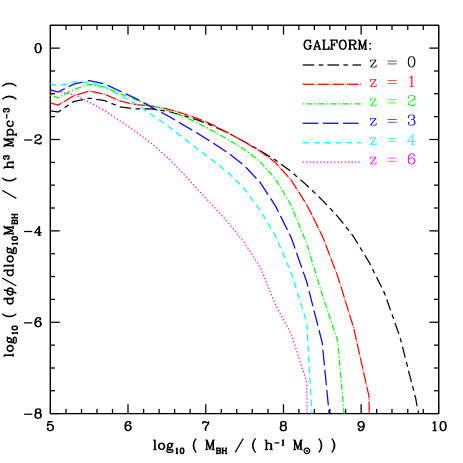
Figure 6: The evolution of the black hole mass function with redshift, as indicated by the key.

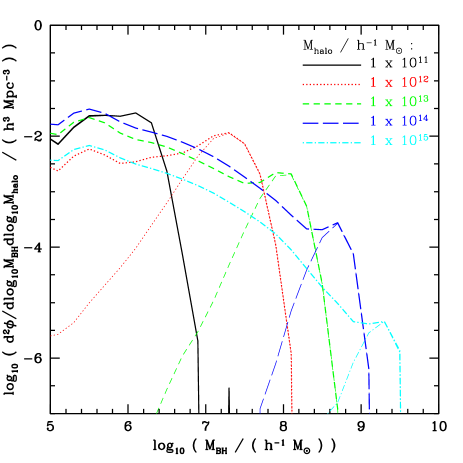
Figure 7: The contribution to the black hole mass function from black holes in dark matter haloes of various masses, as indicated by the key. We show the case for black holes contained within any galaxy (thick lines) and in central galaxies only (thin lines). The black hole mass function for each halo mass is normalized to be the mass function per dex in dark matter halo mass.

4.4 Mass function of progenitor black holes

We now consider the distribution of the masses of black hole progenitors at different epochs for present day black holes. Fig. 8 shows the distribution of progenitor masses at different redshifts, for two ranges of black hole mass measured at $z=0$. The left-hand panel shows the progenitors of $z=0$ black holes with masses in the range $10^{7}-10^{7.5}h^{-1}M_{\odot}$ and the right-hand panel shows the progenitors of $z=$ black holes with masses in the range $10^{9}-10^{9.5}h^{-1}M_{\odot}$. The different line types in the plot show the progenitor mass distributions at different redshifts, as indicated by the key. The distributions plotted are averaged over large numbers of black holes with the appropriate present day mass. In both panels, the $z=0$ distribution is naturally peaked around the present day mass of the black hole.

The evolution of these progenitor mass functions from $z=6$ to $z=1$ looks remarkably similar to that of the universal black hole mass function, albeit truncated at the final $z=0$ black hole mass, and with an overall normalization which increases with increasing final black hole mass.

The similarity of the form and evolution of the progenitor mass functions with those of the universal mass function is remarkable. Only at the lowest progenitor redshift plotted ($z=1$) for black holes with present day masses in the range $10^{7}-10^{7.5}h^{-1}M_{\odot}$ do we see a significant deviation from the form of the overall mass function. The progenitor mass function in this case is rather flat, with fewer low mass black holes and more high mass black holes close in mass to the final black hole. The amplitude of the progenitor mass functions is substantially larger for the black holes with present day mass of $10^{9}-10^{9.5}h^{-1}M_{\odot}$: larger black holes have a significantly larger number of progenitor black holes. This fits in well with our later result (§4.5) that less massive black holes grow primarily by accretion onto a single main branch, whereas black holes larger than $5\times 10^{7}h^{-1}M_{\odot}$ grow primarily by mergers of pre-existing black holes.

Figure 8: The mass functions of progenitor black holes for present day black holes with mass in the interval $10^{7}-10^{7.5}h^{-1}M_{\odot}$ (left panel) and $10^{9}-10^{9.5}h^{-1}M_{\odot}$ (right panel). The distribution of progenitor masses is plotted at different redshifts, as indicated by the key. The mass functions are generated by considering a large sample of black holes at $z=0$, and the normalization is chosen so that each progenitor mass function is the mass function per black hole at $z=0$.

4.5 Black hole growth by mergers and accretion

Figure 9: The cumulative growth with redshift of the black hole mass in the ‘main branch’ divided into the contribution from mergers and accretion. We consider large samples of black holes with $z=0$ masses in the range $10^{7}-10^{7.5}h^{-1}M_{\odot}$ (left) and $10^{9}-10^{9.5}h^{-1}M_{\odot}$ (right). The dotted and dashed lines connect the medians of the distribution, while the 10–90 percentiles of the distribution are shown as errorbars.

We come now to one of the principal results of our paper, the manner in which black holes acquire their mass. There are two distinct modes of mass assembly in our model: “accretion”, in which cold gas is turned into black hole mass during a starburst, and “mergers”, in which existing black holes merge to build a more massive black hole. In the accretion mode, mass is being turned into black hole mass for the first time, whereas in the merger mode, pre-existing black hole mass is being rearranged or reassembled into a more massive black hole. In Fig. 9, we plot the fraction of the mass in the ‘main branch’ which is assembled by mergers or gas accretion as a function of redshift. We show results for black holes in two mass ranges at redshift zero: $10^{7}-10^{7.5}h^{-1}M_{\odot}$ (left) and $10^{9}-10^{9.5}h^{-1}M_{\odot}$ (right). Fig. 9 shows that at high redshifts, growth by accretion dominates over growth through mergers. Mergers become increasingly important as redshift decreases, but for the $10^{7}-10^{7.5}h^{-1}M_{\odot}$ black holes, the cumulative growth by mergers never exceeds the cumulative growth by accretion, even at redshift zero. However, for black holes of mass $10^{9}-10^{9.5}h^{-1}M_{\odot}$ at $z=0$, the cumulative growth of their main progenitors by mergers exceeds that by accretion around a redshift of 1.7, and growth by accretion almost halts after this. By redshift zero, the cumulative mass assembled by mergers greatly exceeds that assembled by accretion. The declining importance of growth by accretion for black holes of mass $>10^{7.5}h^{-1}M_{\odot}$ reflects the decline in the amount of gas available in mergers as more and more of the gas in collapsed haloes is consumed into stars.

In Fig. 10, we plot the fraction of the mass of black holes which, by $z=0$ (left) and $z=2$ (right), has been accumulated by mergers or accretion onto the ‘main branch’. This is shown as a function of black hole mass. Fig. 10 (left) shows that, by redshift zero, low mass black holes have accumulated nearly all of their mass by direct accretion onto a single ‘main branch’, while the most massive black holes accumulate 80–90% of their mass by mergers of less massive black holes onto the ‘main branch’. The transition from accretion-dominated growth to merger-dominated growth occurs at a $z=0$ mass of just over $10^{8}h^{-1}M_{\odot}$. Fig. 10 (right) shows that at $z=2$, all black holes, even those more massive than $10^{8}h^{-1}M_{\odot}$, grow predominantly by accretion, although there is a contribution from mergers which increases with black hole mass. Comparison of the results in Fig. 10 for $z=0$ and $z=2$ shows that for any given black hole mass, growth by accretion is more significant for a black hole at $z=2$ than at $z=0$, and that this difference is greater for the more massive black holes. This is consistent with the idea that the luminous growth (i.e. growth by direct accretion of gas) of higher mass black holes switches off towards lower redshifts (see §6).

Figure 10: The cumulative fraction of the mass assembled by mergers and accretion, as a function of final black hole mass at $z=0$ (left) and $z=2$ (right). The medians are connected by lines, and the 10–90 percentile spread of the distribution is shown as an errorbar for each black hole mass.

4.6 The redshift of black hole formation

In Fig. 11 we show the formation redshifts of black holes, binned by $z=0$ mass. Each of the six panels corresponds to a different definition of formation redshift. ‘Formation’ is defined as the time when either the main progenitor (right three panels) or the sum of all existing progenitor black holes (left three panels) first exceeds a given fraction of the final black hole mass. Where the formation redshift is defined as the time when the main progenitor first exceeds a given fraction of the final mass, we refer to this as the mass assembly redshift, since this is the redshift where the stated fraction of the mass has been assembled into a single object. Where the formation redshift is defined as the time when the sum of all progenitors first exceeds a given fraction of the final mass, we refer to this as the mass transformation redshift. This distinction between the mass transformation time and mass assembly time for black holes is analagous to that between the star formation time and stellar mass assembly time for the stars in a galaxy. We consider three different mass fraction thresholds to define formation times: 0.01 (top), 0.5 (middle) and 0.95 (bottom).

When we consider the assembly of 50% or 95% of the final black hole mass (Fig. 11 – middle-right & bottom-right), we see clear hierarchical behaviour; the more massive black holes at redshift zero peak in their formation times at lower redshift than the less massive ones. This is evidence for the hierarchical assembly of black hole mass into a single final object. However, when we consider the redshift at which 50% of the final black hole mass has accreted onto any black hole in the merger tree (Fig. 11 – middle-left), we see the opposite trend; in the mass range $M_{\rm BH}=10^{7}-10^{9.5}h^{-1}M_{\odot}$, the more massive black holes display a distribution of formation redshifts which peaks at higher redshift. When we consider the redshift at which 95% of the final black hole mass is accreted onto any black hole in the merger tree (Fig. 11 – bottom-left), we see further evidence of downsizing. Although the formation rate peaks at a similar redshift ($z\sim 1.2$) for all black holes in the mass range $M_{\rm BH}=10^{7}-10^{9.5}h^{-1}M_{\odot}$, the decline in the fraction forming per unit time as redshift approaches zero is far steeper for more massive black holes within this mass range. The observational evidence for “downsizing” refers to the accretion of mass onto a particular progenitor, which is accompanied by the release of energy. Hence, it is the latter trend which is relevant – as black hole mass increases, the redshift when mass is accreted onto any progenitor increases. We return to this point in §6.

We consider now the early growth of the black holes. Fig. 11 (top-left) shows the redshift when the first 1 per cent of the final black hole mass has collapsed into any of the branches of the merger tree. There is a clear trend for larger black holes to be seeded earlier. This is also a form of downsizing. All of the black holes in our largest mass bin ($M_{\rm BH}=10^{9}-10^{9.5}h^{-1}M_{\odot}$) and many of those in the next mass bin, $M_{\rm BH}=10^{8}-10^{8.5}h^{-1}M_{\odot}$, are seeded before reionization occurs in the model at $z=6$. Another interesting feature of Fig. 11 is that, for almost any definition of formation time, less massive black holes have a much wider spread in formation times than more massive black holes.

There is little difference in the distribution of formation times of black holes of mass $M_{\rm BH}=10^{5}-10^{6.5}h^{-1}M_{\odot}$ regardless of whether we use a definition which relates to the ‘main branch’ or to ‘all progenitors’. This follows from our earlier result that black holes in this mass range formed almost exclusively by accretion onto a single object, with little contribution from mergers between black holes (§4.5, Fig. 10). The differentiation between the different definitions of formation time begins to become apparent for black holes of mass $M_{\rm BH}=10^{7}-10^{7.5}h^{-1}M_{\odot}$ and is increasingly more significant as black hole mass increases further. This relates to our earlier result that the contribution to the final black hole mass from mergers of pre-formed black holes compared to the contribution from direct cold gas accretion onto the main branch increases strongly with increasing black hole mass (§4.5, Fig. 10).

Figure 11: The distribution of formation redshifts of black holes in 5 different bins of $z=0$ mass, as indicated by the key. The differing definitions of formation redshift used in each of the six plots are noted briefly on each plot and explained more fully in §4.6 of the text.

4.7 Black hole merger rates

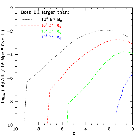
Figure 12: Black hole merger rate per unit time as a function of redshift. The merger rate is plotted for 5 different mass thresholds, as shown by the key, which the (pre-starburst) masses of both black holes must exceed.

We show the merger rate per unit time of black holes as a function of redshift in Fig. 12. We show this for a number of mass thresholds which must be exceeded by both of the black holes that take place in the merger. The merger rates peak at lower redshift for more massive black holes, with the merger rate for the most massive bin still rising at $z=0$. This is consistent with the trend seen at $z=0$ that larger mass black holes grow primarily by mergers, while less massive black holes grow primarily by accretion (§4.5).

This behaviour in the growth and merging of black holes of varying mass is largely a reflection of the general hierarchical growth of structure, moderated in the case of galaxies and black holes by baryonic processes. The results presented in this subsection concern only mergers of black holes, not necesarily their total growth which can also involve accretion. There is no evidence for ‘anti-hierarchical’ behaviour in the evolution of black hole mergers. However, as we show in §6, this is perfectly compatible with quasar downsizing – black hole merging can be a ‘dark’ process in which no gas is present, whereas the observational evidence for downsizing refers to processes involving star formation or gas accretion.

4.8 The fraction of baryons in black holes

Having considered the formation of individual black holes, we now look at the global picture. In Fig. 13, we show the integrated cosmic density of all the baryonic components of the universe; hot gas, cold disc gas, stars and black holes. After $z\sim 4$, the growth of black hole mass in the universe slows down in comparison to that of stars, as quiescent star formation begins to dominate over star formation in bursts. The decline in cold gas from redshift 2 to 0 goes a small way towards explaining the decline in quasar activity over this redshift interval. The decline in the galaxy merger rate and the transition from burst-dominated star formation to quiescent star formation also play a role. In Fig. 14, we show the star formation rate, divided into burst and quiescent modes, and the rate of black hole growth. By construction in our model, black hole growth is more strongly correlated with the star formation rate in bursts than with star formation in general. Very broadly, although perhaps less so at low redshifts, black hole accretion tracks the overall star formation over cosmic time, as observed ([1998]).

The cosmological mass density of black holes at $z=0$ is a quantity of interest. In our model, we find that $\rho_{\rm BH}=2.83\times 10^{5}M_{\odot}\rm Mpc^{-3}$. Observationally, $\rho_{\rm BH}$ is determined by integrating the black hole mass function which, in turn, is inferred from a combination of the velocity dispersion distribution of galaxies, the K-band luminosity function or the bulge stellar mass function, and the appropriate $M_{\rm BH}-\rm bulge$ relation. Observed values of $\rho_{\rm BH}/(10^{5}M_{\odot}\rm Mpc^{-3})$, converted to $H_{0}=70{\rm kms}^{-1}{\rm Mpc}^{-1}$, are : $2.9\pm 0.5$ ([2002]), $2.4\pm 0.8$ ([2002]), $2.8\pm 0.4$ ([2004]), $4.2\pm 1.1$ ([2004]) and $4.6^{+1.9}_{-1.4}$ ([2004]). Our estimate is towards the lower end of the broad range spanned by the observational estimates. We do not include any measurement errors in our estimate. A detailed comparison would need to take into account galaxy type (some estimates are based only on ellipticals), the flux limits of the observational samples and the treatment of the dispersion in the $M_{\rm BH}-\rm bulge$ relations when converting from bulge properties to black hole masses. Many observational estimates assume that the scatter in $\rm log(M_{\rm BH})$, at a given value of the bulge property under consideration, is symmetrical. This assumption then leads to larger values of $\rho_{\rm BH}$ for larger assumed values of the scatter ([2004]). However, it is not at all clear that the scatter in these relations is symmetrical.

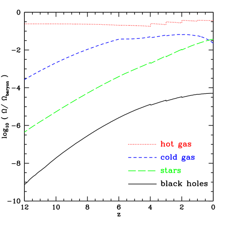
Figure 13: The evolution of the fraction of the baryons in the universe in hot gas, cold gas, stars (disc plus bulge) and black holes. The small abrupt changes in some of the lines are due to simulation runs that finish at different times.

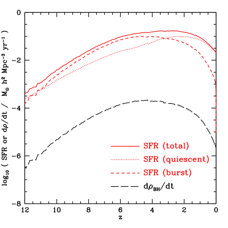
Figure 14: The variation with redshift of the global star formation rate (starbursts, quiescent and total) and the global rate of black hole growth.

5 The evolution of the relation between black hole mass and bulge properties.

Figure 15: The redshift evolution of the relations between central black hole mass, $M_{\rm BH}$, and bulge properties. Each panel shows the relationship between $M_{\rm BH}$ and a different property of the host spheroid : (a) the bulge rest-frame B-band magnitude; (b) the bulge rest-frame K-band magnitude; (c) the stellar mass of the bulge; (d) the velocity dispersion of the bulge. The model predictions are shown by the symbols with errorbars; the lines show the median relations and the errorbars the 10–90 percentile spread of the distributions. Redshifts 0, 1, 2, 3, 4 and 6 are shown in different line types, as indicated by the key.

In this section, we discuss the evolution of the relationship between black hole mass and various galaxy bulge properties: K-band and B-band bulge magnitude, bulge stellar mass and bulge velocity dispersion. We show these relationships in Fig. 15, in each case plotting the model predictions for the $M_{\rm BH}-\rm bulge$ relationships at $z=0,1,2,3,4$ and  6. We discuss each of these in turn, briefly referring to any relevant observational data. However, it is difficult to make rigorous comparisons to current data. While relationships between black hole mass and bulge properties are fairly well determined at $z=0$, this is currently not the case for $z>0$, where observational samples are small and subject to selection effects. In particular, different surveys sample the population of galaxies and, where relevant, the AGN subpopulation, in ways that are not always straightforward to replicate in the models.

We show our model predictions for the $M_{\rm BH}-M_{\rm B,bulge}$ relation in Fig. 15(a) and the $M_{\rm BH}-M_{\rm K,bulge}$ relation in Fig. 15(b). In the model, these relationships shift towards brighter magnitudes at higher redshifts. This is a reflection of the evolving stellar populations. The stellar populations of bulges at low redshift are older and thus less luminous than their high redshift counterparts. This effect more than compensates for any evolution in the opposite direction in the $M_{\rm BH}-M_{\rm bulge}$ relation, which we discuss below. The redshift evolution in the $M_{\rm BH}-M_{\rm B,bulge}$ relation is greater than that in the $M_{\rm BH}-M_{\rm K,bulge}$ relation because stellar populations dim more strongly with time in the B-band than in the K-band. Observationally, however, Peng et al. ([2006]), selecting high redshift quasars, find little trend in the $M_{\rm BH}-M_{\rm R,bulge,rest}$ relation with redshift, which conflicts somewhat with our prediction of an evolution towards brighter magnitudes as redshift increases.

We show the $M_{\rm BH}-M_{\rm bulge}$ relation in Fig. 15(c). There is no significant evolution in either the slope or scatter at large bulge masses. For $M_{\rm bulge}<10^{10}h^{-1}M_{\odot}$, the black hole mass to bulge mass ratio increases with increasing redshift. Observationally, Peng et al. ([2006]) find that the ratio of $M_{\rm BH}$/$M_{\rm bulge}$ was 3–6 times larger at $z\gtrsim 2$ for AGNs than for quiescent galaxies at $z=0$. McLure et al. ([2006]), selecting radio galaxies at $z>0$ from the 3CRR catalogue, argue that $M_{\rm BH}$/$M_{\rm bulge}$ increases with redshift, and is $\sim 4$ times greater for radio galaxies at $z=2$ than for quiescent galaxies at $z=0$. We find that $M_{\rm BH}$/$M_{\rm bulge}$ was $\sim$ 2 times greater at $z=2$ than at $z=0$ for $M_{\rm bulge}<10^{10}h^{-1}M_{\odot}$. This evolution is in the same sense as and of comparable size to the observational trend, although the effect in the model is perhaps not as strong. As discussed in §3.1, the predicted variation in the $M_{\rm BH}$/$M_{\rm bulge}$ ratio reflects the variation in the fraction of bulge stars which formed quiescently in discs. Mergers at higher redshift, when discs are more gas-rich and have fewer stars, deposit a lower fraction of (quiescently-formed) disc stars in the bulge (e.g. [2006]).

Close inspection of Fig. 15(c) shows that a few objects at the highest redshifts have black hole masses that exceed $F_{\rm BH}\times M_{\rm bulge}$. This would appear to be impossible given our definition of $F_{\rm BH}$ in §2.3. This apparent anomaly is due to our assumption that the mass of the black hole increases instantaneously at the time of the starburst. In our model, star formation in the bursts extends over $\sim 50$ dynamical times, while quasars shine only over $\sim 0.3$ dynamical times, so that the stellar mass builds up much more slowly than the black hole mass. It seems likely, however, that a black hole will still be growing towards its final mass towards the end of the starburst ([2002, 2005, 2005]). We defer a study of the co-evolution of the stars and the the black hole mass to future work.

Finally, we show the $M_{\rm BH}-\sigma_{\rm bulge}$ relation in Fig. 15(d). There is no evolution in the slope of the relation, but the zeropoint does evolve and the scatter increases significantly towards higher redshift. For a given mass of black hole, the velocity dispersion of the bulge is greater at higher redshift. To some extent, this evolution reflects the expected variation in the properties of dark matter haloes: at a given mass, the halo velocity dispersions scales as $\sigma\propto(z_{\rm form}+1)^{1/2}$. Alternatively, the evolution could be viewed as a reduction in the black hole mass with increasing redshift, for a fixed bulge velocity dispersion.

Shields et al. ([2003]) have compared the relative amounts of black hole mass in distant quasars and in galaxies in the local Universe. They find a large scatter and an increase of $0-0.5~{}\rm dex$ in $M_{\rm BH}/\sigma_{\rm bulge}$ between $z=0$ and $z\sim 3$. Similarly, Woo et al. ([2006]) have compared Seyferts at $z=0.36$ with galaxies at $z=0$. They too find an increase, of $0.62\pm 0.10~{}\rm dex$, in black hole mass at fixed $\sigma_{\rm bulge}$ at $z=0.36$ compared to $z=0$. Thus, the observed trend in $M_{\rm BH}/\sigma_{\rm bulge}$, if any, is in the opposite direction to the trend we find in our simulations. It is possible that our model neglects effects that would cause black holes to be a larger fraction of the galactic bulge mass at higher redshifts. However, it must be remembered that $\sigma_{\rm bulge}$ is one of the more uncertain properties of the galaxies in our model and that dynamical effects which are not included could play a role in determining the properties of merger remnants ([2006, 2006]).

6 Downsizing in a hierarchical universe

In cosmology, “downsizing” is an ill-defined term which has been applied to describe the phenomenon whereby luminous activity (e.g. star formation or accretion onto black holes) appears to be occuring predominantly in progressively lower mass objects (galaxies or BHs) as the redshift decreases. Claims of downsizing were first made in connection with the population of star-forming galaxies ([1996]). More recently, the same trend has been inferred from the evolution of the X-ray luminosity function of quasars ([2003, 2003, 2003, 2005, 2005]): the number of bright X-ray sources peaks at a higher redshift than the number of faint X-ray sources. The optical quasar luminosity function shows similar evolution, with more bright objects seen at increasing redshifts (e.g. [2004]).

The apparent downsizing in the quasar X-ray luminosity function has been interpreted by some authors as implying that black holes acquire mass in an ‘anti-hierarchical’ manner ([2004, 2004, 2004, 2005]). In this Section, we demonstrate that the “downsizing” of the luminous growth of black holes is actually a natural feature of our model, despite the fact that the overall assembly of mass into black holes is hierarchical. Downsizing in the galaxy population in hierarchical models is promoted by the earlier collapse and more active merging of objects in regions of high overdensity ([1995, 2006, 2006]). In recent models of galaxy formation, this natural trend is accentuated by the feedback processes associated with AGN activity in massive haloes (Bower et al. 2006; Croton et al. 2006). However, we wish to emphasize that AGN activity in low redshift cooling flows is very far from being the only ingredient required for downsizing, and that we still find downsizing in our model. We now review some of the indirect evidence already presented in support of this conclusion (§6.1), and go on to present explicit predictions which reveal which black holes in our model are accreting mass most rapidly (§6.2).

6.1 Indirect evidence for downsizing in the model: the evolution of the optical luminosity function

The optical quasar luminosity function, as we have already remarked, reveals a dramatic increase in the space density of bright quasars with increasing redshift ([2004]). In §3.2, we presented the model predictions for the optical luminosity function, which are in good agreement with this trend in the observations. Two features of our model are responsible for this success: the increase in the halo merger rate (and hence the galaxy merger rate) with increasing redshift and the increase in the gas content of discs with increasing redshift (see also [2000]). In combination, these phenomena lead to an increase in the frequency and strength of starbursts with redshift. In our model, a starburst results in a luminous phase of growth of the supermassive black hole; a fraction $F_{\rm BH}$ of the cold gas which is turned into stars during the burst is accreted onto the black hole.

Galaxy mergers are still an important way of building black hole mass at low redshift. Our model predicts that BH-BH mergers are the most important channel for building black hole mass for the most massive black holes at the present day. This dark growth process represents the assembly of mass which is already locked up in black holes into larger units. Galaxy mergers at low redshift tend to be gas poor in our model simply because more time has elapsed to allow galactic discs to turn cold gas into stars quiescently. This effect is accentuated in the case of the most massive black holes which tend to reside in the more massive dark haloes. The process of galaxy formation starts earlier in the progenitors of massive haloes, since these objects collapse into bound structures earlier than is the case in less extreme environments.

6.2 Direct evidence for downsizing in the model: which black holes are accreting mass?

Our model allows us to separate the mass assembly of black holes into two contributions: accretion, in which cold gas is turned into black hole mass in a starburst and mergers, in which existing black holes merge to build a more massive black hole. Here we focus on the process of gas accretion. Fig. 16 presents two views showing which mass of black holes are accreting material the most vigorously. The left-hand panels of Fig. 16 show the distribution of accretion rates, expressed in units of the Eddington mass accretion rate. Since the Eddington accretion rate scales with mass, this is easily scaled to give the distribution of fractional accretion rates. The right-hand panels compare the present accretion rate to the past average accretion rate (calculated as $\langle\dot{M}\rangle\times~{}t_{\rm age\thinspace of\thinspace Universe}/\langle M_{\rm BH}\rangle$, as a function of black hole mass. Each row corresponds to a different redshift (top: $z=0$, middle: $z=1$, bottom $z=2$). In these plots, we have not limited the mass accretion rate to be less than or equal to the Eddington limit.

The left-hand side of Fig. 16 shows that, at all redshifts, there is a large spread in the Eddington ratios at which black holes are accreting. There is variation amongst mergers in gas supply, accretion timescale and initial black hole mass. Furthermore, the Eddington ratio evolves during any single accretion event. As expected, the mass accretion shifts towards higher fractions of the Eddington limit at higher redshift since there is more gas available in mergers. At $z=0$, we see that as black hole mass increases, accretion shifts to lower fractions of the Eddington ratio. This trend is less pronounced at $z=1$ and practically disappears by $z=2$. Thus, more massive black holes were accreting mass more rapidly at $z=2$ than they are today. The predicted distribution of mass accretion rates at $z=0$ agree reasonably well with the observational results of Heckman et al. ([2004]). The distribution is normalized to unit area, but most black holes, particularly at lower redshifts, are not accreting at all (i.e. they are in a $\delta$-function at $\dot{M}=0$).

The right-hand column of Fig. 16 shows the ratio of the present accretion rate to the past average accretion rate ($\thinspace\langle\dot{M}\rangle\times~{}t_{\rm age}/\langle M_{\rm BH}\rangle\thinspace$) as a function of black hole mass at $z=$ 0, 1 and 2. If this ratio exceeds unity, then the current mass accretion rate exceeds the average rate at which the black hole gained mass in the past (summed over all progenitors). The predictions for this ratio are sensitive to the black hole selection, for example, selection using a cut in quasar luminosity. We show results for all black holes (solid lines) and also for black holes selected as quasars brighter than a given luminosity. Note that the bulk of black holes in the model are not accreting material at any given time. The solid lines in each panel show that there is clear evidence for downsizing in the model. At $z=0$, more massive black holes are growing less rapidly than less massive black holes. By $z=1$, this trend is greatly diminished, and at $z=2$ it is reversed, i.e. the most massive black holes have the highest fractional accretion rate. When only quasars are selected, those with low mass black holes show similar fractional accretion rates as redshift varies from 0 to 2, while quasars with massive black holes show a strong decline in fractional accretion rate towards the present day.

Figure 16: Left panels: The distribution of accretion rate normalized by the Eddington mass accretion rate. Right panels: the current mean mass accretion rate normalized by the past average mass growth rate, plotted against black hole mass. In both cases, each row corresponds to a different redshift: $z=0$ (top), $z=1$ (middle) and $z=2$ (bottom). In the left hand panels, each line shows the distribution of accretion rates for black in the mass interval shown by the key. In the right hand panels, the lines correspond to different cuts on quasar luminosity, again as shown by the key.

7 Summary and Discussion

We have described an extension to the GALFORM semi-analytical model of galaxy formation in the $\Lambda$CDM cosmology to track the growth of black holes (BH). Our model for black hole growth has one free parameter, $F_{\rm BH}$, the mass accreted onto the black hole as a fraction of the stellar mass produced during a starburst. We set the value of $F_{\rm BH}$ so as to reproduce the zeropoint of the present day $M_{\rm BH}-\rm bulge$ relations. The slope, scatter and evolution of the $M_{\rm BH}-\rm bulge$ relations are model predictions.

In our model, black holes grow only during and following a galaxy merger. They grow through two distinct channels: mergers of pre-existing black holes and accretion of cold gas if a starburst is triggered by the merger. The importance of growth through black hole mergers increases with the mass of the black hole; at $z=0$ the growth of black holes less massive than $5\times 10^{7}h^{-1}M_{\odot}$ is dominated by accretion, while the growth of more massive black holes is dominated by mergers. In general, the growth of black hole mass by mergers becomes more important at low redshifts as the supply of gas available for accretion is consumed by star formation. Our model neglects black hole growth from gas accreted directly in a cooling flow from a hot gas reservoir, as may be expected in massive haloes at late times. This is the “feedback mode” of black hole growth invoked by Bower et al. ([2006]) in their model that explains why there is an exponential cutoff at the bright end of the galaxy luminosity function. Apart from this new growth channel and an explicit treatment of disc instabilities, the calculation of black hole growth in the Bower et al. model is very similar to ours. However, around 20% of the global mass in black holes in the Bower et al. study is due to the “feedback mode” of growth. It is as important as mass assembly due to galaxy mergers for the most massive black holes, which accumulate $\sim 50\%$ of their mass via this channel (Richard Bower, priv. comm.).

Essentially all current observational estimates of the accumulation of black hole mass are sensitive to luminous growth, i.e. mass accretion. However, we predict that the importance of growth through BH-BH mergers grows with decreasing redshift and with increasing black hole mass. BH-BH mergers represent a dark mode of growth that is more difficult to observe and confirm. The most obvious way to detect BH-BH mergers is through the emission of gravitational waves (e.g. [1994]). This may be possible in ten years with the planned LISA gravitational wave interferometer. When gas is present during a black hole merger, a circumbinary accretion disc could form and the BH merger may produce high velocity gas outflows ([2002]) followed by an X-ray afterglow which could be detected by the next generation of X-ray observatories ([2005]). Winged or X-shaped radio sources ([2002]) and cores in elliptical galaxies ([1997, 2002]) may be indirect evidence of gas-poor mergers.

Our model predicts that the most important growth mechanism for the most massive black holes is the “dark” mode or mass assembly through BH mergers. A testable prediction of our model is that a tail of black holes with masses above a few times $10^{9}M_{\odot}$ should be found at $z=0$ once high quality observations covering a large volume of the local Universe become available (§4.2). Furthermore, we expect that these will be more massive than any found in quasars at high redshift. To date, only black holes less massive than $\sim 3\times 10^{9}M_{\odot}$ have been unambiguously observed in galaxies at $z=0$ ([2002]) and in luminous, optically-selected quasars over the redshift interval $0<z<2$ ([2004]). However, this implied limit on black hole mass is far from robust. The most massive black holes at $z=0$ tend to reside in massive and hence rare elliptical galaxies, which could easily have been missed in existing surveys. Larger volumes ($\gtrsim$ a few times $10^{6}h^{-3}\rm Mpc^{3}$) need to be surveyed to find such objects, which are therefore likely to lie at large distances. This, coupled with their expected low surface brightness (more massive ellipticals tend to have lower surface brightness cores), could make it difficult to measure their central mass using methods based on stellar dynamics ([2001]). The high redshift quasar data do not give a complete census of the black hole populations, as quasar observations are only able to probe accreting black holes.

There is an important distinction to be made in our model between mass transformation and mass assembly. Mass transformation refers to the process of turning cold gas into black hole mass; at any one time in the formation history of a black hole, this phenomenon could be occuring across a number of progenitor black holes. Mass assembly refers to the accumulation of mass in a black hole’s main progenitor, and may occur via both direct accretion of gas and merging of pre-existing black holes. Black hole mass assembles hierarchically; more massive black holes are assembled at lower redshifts than less massive black holes. However, if we choose to define the formation time of a black hole in terms of the mass transformation redshift when some fraction of its mass has been accreted onto any progenitor, we find that, for $M_{\rm BH}>10^{7}h^{-1}M_{\odot}$, more massive black holes form earlier. This dichotomy mirrors the growth of stellar mass in galactic spheroids in hierarchical models. In the semi-analytical models, galaxy mergers produce spheroids. At high redshift, the mergers tend to be gas rich and new stars are produced as a result of the merger event. At low redshift, galactic discs tend to be gas poor and consist mainly of stars, with the result that the merger simply rearranges the pre-existing stars ([1996, 1996, 2006, 2006]).

While we find that black hole mass is assembled hierarchically, our model clearly exhibits a “downsizing” in the mass of black holes which are undergoing luminous accretion. At the present day, we find that low mass black holes are accreting material at a higher proportion of their Eddington luminosity than high mass black holes. This distinction is less apparent at higher redshifts. Another way to demonstrate this downsizing is to examine the rate at which black holes are accreting mass, expressed as a fraction of the mass already in place: $\langle\dot{M}_{\rm BH}\rangle/\langle M_{\rm BH}\rangle$. At $z=0$, $\dot{M}_{\rm BH}/M_{\rm BH}$ is largest for low mass black holes and drops rapidly with increasing mass. This trend is removed with increasing redshift; accretion becomes an increasingly important mode of mass assembly for all masses of black hole at earlier epochs in the universe.

A number of authors have claimed that black holes grow in an “anti-hierarchical” fashion ([2004, 2004, 2004]). This conclusion is reached by comparing an inferred present day black hole mass function with the black hole mass function expected from AGN relics under the assumption that black holes grow exclusively by accretion. These calculations ignore any contribution to the mass of black holes arsising from BH-BH mergers. Furthermore, the assumption that all black holes accrete at a constant fraction of their Eddington ratio ([2004, 2004]), or the use by Merloni ([2004]) of the ‘fundamental plane of black hole activity’ ([2003]), which has a very large scatter, will introduce errors that may become cumulatively very large as the black hole mass function is integrated backwards in time.

While the zeropoints of the present day $M_{\rm BH}-\rm bulge$ relations are set by adjusting a single free parameter, the slope, scatter and evolution of these relations are genuine predictions of the model. We find little evolution with redshift in the slope of any of the $M_{\rm BH}-\rm bulge$ relations, although our model predicts differing evolution in their zeropoints, depending upon which particular bulge property is being considered. If we focus attention on a fixed black hole mass, we find that with increasing redshift, the typical host bulge is more luminous in the rest-frame B-band and K-band, shows little change in stellar mass (except in the case of low mass black holes, where the stellar mass is lower) and has a somewhat higher velocity dispersion.

Our model predicts the presence of massive black holes at high redshift. However, our simulations are not large enough to check if a population of sufficiently massive black holes has formed at high redshift to account for observations of quasars that have been interpreted as implying the presence of very massive black holes at early times (Fan et al. 2001, 2004). Fan et al. have discovered quasars of magnitude $M_{1450}\sim-27$ at $z\sim 6$, albeit at a low space density, $\phi\approx 1.6\pm 0.5\times 10^{-10}h^{3}\rm Mpc^{-3}$ ([2004]). Assuming that these objects are radiating at the Eddington luminosity with an Elvis et al. ([1994]) spectrum, and that beaming and gravitational lensing are insignificant, Fan et al. ([2001]) inferred that these quasars host black holes masses of $\sim 1-3\times 10^{9}h^{-1}M_{\odot}$. In this paper, we probe the mass function of $z=6$ black holes only down to a space density of $\phi\sim 1\times 10^{-8}h^{3}\rm Mpc^{-3}$, which is not sparse enough to compare with these data. We plan to address this problem by performing simulations of a larger volume than those analyzed here, which will probe the high mass end of the halo mass function in detail.

In summary, we have presented a new model for the concurrent growth of galaxies and black holes in the $\Lambda$CDM cosmology. We have previously shown that this model can successfully account for many observed properties of the galaxy population over a large range of wavelengths, from the local optical and infrared galaxy luminosity function to the number counts of submillimeter galaxies and the UV luminosity function of Lyman-break galaxies at redshift $z\sim 3$ (Baugh et al. 2005). In this paper we have focussed on the properties of the black hole population that grows in unison with the spheroidal component of the galaxies. This model can account for a variety of observables that involve black holes, such as the relationship between the mass of the central black hole in galaxies and the properties of the bulge, the quasar luminosity function, and the apparent “anti-hierarchical” growth of black holes. The model may be tested by future observations of the evolution of the $M_{\rm BH}-\rm bulge$ relations and, perhaps, by the detection of gravitational waves associated with the mergers of massive black holes that play a prominent role in our model.

8 Acknowledgements

We thank Andrew Benson, Richard Bower, Marta Volonteri, Darren Croton, Gregory Novak and the anonymous referee for useful comments and discussions and John Helly for providing tree-plotting routines. We are indebted to Lydia Heck for providing extensive help with computing and for maintaining the PC cluster on which the calculations in this paper were performed. RKM was supported by a PPARC studentship. CMB is supported by the Royal Society. CSF is a Royal Society-Wolfson Research Merit Award holder. This research was supported by the PPARC rolling grant.

References

- [2003] Alexander D.M., Bauer F.E., Brandt W.N., Hornschemeier A.E., Vignali C., Garmire G.P., Schneider D.P., Chartas G., Gallagher S.C., 2003, AJ, 125, 383
- [2005] Alexander D.M., Smail I., Bauer F.E., Chapman S.C., Blain A.W., Brandt W.N., Ivison R.J., 2005, Nature, 434, 738
- [2002] Aller M.C., Richstone D., 2002, AJ, 124, 3035
- [2007] Almeida C., Baugh C.M., Lacey C.G., 2007, MNRAS, 376, 1711
- [2002] Archibald E.N., Dunlop J.S., Jimenez R., Friaça A.C.S., McLure R.J., Hughes D.H., 2002, MNRAS, 336, 353
- [2002] Armitage P.J., Natarajan P., ApJ, 567, 9
- [2002] Baker J., Campanelli M., Lousto C.O., Takahashi R., 2002, PhRvD, 65, 124012
- [2004] Baker J., Campanelli M., Lousto C.O., Takahashi R., 2004, PhRvD, 69, 027505
- [2005] Barger A.J., Cowie L.L., Mushotzky R.F., Yang Y., Wang W.-H., Steffen A.T., Capak P., 2005, AJ, 129, 578
- [2006] Baugh C.M., 2006, Rep. Prog. Phys., 69, 3101.
- [1996] Baugh C.M., Cole S., Frenk C.S., 1996, MNRAS, 283, 1361
- [2005] Baugh C.M., Lacey C.G., Frenk C.S., Granato G.L., Silva L., Bressan A., 2005, MNRAS, 356, 1191
- [1978] Begelman M.C., 1978, MNRAS, 184, 53
- [2002] Begelman M.C., 2002, ApJ, 586, L97
- [2006] Bell E.F. et al. , 2006, ApJ, 640, 241
- [2002] Benson A.J., Lacey C.G., Baugh C.M., Cole S., Frenk C.S., 2002, MNRAS, 333, 156
- [2003a] Benson A.J., Frenk C.S., Baugh C.M., Cole S., Lacey C.G., MNRAS, 2003a, 343, 679
- [2003b] Benson A.J., Bower R.G, Frenk C.S., Lacey C.G., Baugh C.M., Cole S., 2003, ApJ, 599, 38
- [2005] Borys C., Smail I., Chapman S.C., Blain A.W., Alexander D.M., Ivison R.J., 2005, ApJ, 635, 853
- [2006] Bower R.G., Benson, A.J., Malbon, R., Helly, J.C., Frenk, C.S., Baugh, C.M., Cole, S., Lacey, C.G., 2006, MNRAS, 370, 645
- [1998] Boyle B.J., Terlevich R.J., 1998, MNRAS, 293, 49
- [2004] Bromley J.M., Somerville R.S., Fabian A.C., 2004, MNRAS, 350, 456
- [2003] Bromm V., Loeb A., 2003, ApJ, 596, 34
- [2001] Cattaneo A., 2001, MNRAS, 324, 128
- [2005a] Cattaneo A., Combes F., Colombi S., Bertin E., Melchior A.-L., 2005a, MNRAS, 359, 1237
- [2005b] Cattaneo A., Blaizot J., Devriendt J., Guiderdoni B., 2005b, MNRAS, 364, 407
- [2004] Chapman S.C., Smail I., Windhorst R., Muxlow T., Ivison R.J., 2004, ApJ, 611, 732
- [2000] Cole S., Lacey C.G., Baugh C.M., Frenk C.S., 2000, MNRAS, 319, 168
- [2001] Cole S. et al. , 2001, MNRAS, 326, 255
- [2004] Collin S., Kawaguchi T., 2004, A&A, 426, 797
- [1996] Cowie L.L., Songaila A., Hu E., Cohen J.G., 1996 AJ, 112, 839
- [2003] Cowie L.L., Barger A.J., Bautz M.W., Brandt W.N., Garmire G.P., 2003, ApJ, 584, 57
- [2004] Croom S.M., Smith R.J., Boyle B.J., Shanks T., Miller L., Outram P.J., Loaring N.S., 2004, MNRAS, 349, 1397
- [2006] Croton D.J., 2006, MNRAS, 369, 1808
- [2006] Croton D.J. et al. , 2006, MNRAS, 365, 11
- [2006] Dekel A., Cox T.J., 2006, MNRAS, 370, 1445
- [2006] De Lucia G., Springel V., White S.D.M., Croton D., Kauffmann G., 2006, MNRAS, 366, 499
- [2005] Di Matteo T., Springel V., Hernquist L., 2005, Nat, 433, 604
- [2003] Dunlop J.S, McLure R.J, Kukula M.J, Baum S.A, O’Dea C.P, Hughes D.H., 2003, MNRAS, 340, 1095
- [ 1988] Efstathiou G., Rees M.J., 1988, MNRAS, 230, 5
- [2004] Eke V.R. et al. , 2004, MNRAS, 355, 769
- [1994] Elvis M. et al. , 1994, ApJS, 95, 1
- [2003] Enoki M., Nagashima M., Gouda N., 2003, PASJ, 55, 133
- [1997] Faber S.M. et al. , AJ, 114, 1771
- [2001] Fan X. et al. , 2001, AJ, 121, 54
- [2004] Fan X. et al. , 2004, AJ, 128, 515
- [2004] Favata M., Hughes S.A., Holz D.E., 2004, ApJ, 607, 5
- [2000] Ferrarese L., Merritt D., 2000, ApJ, 539, 9
- [1983] Fitchett M.J., 1983, MNRAS, 203, 1049
- [2000] Gebhardt K. et al. , 2000, ApJ, 539, 13
- [2007] Gilli R., Comastri A., Hasinger G., 2007, A&A, 463, 79
- [2000] Granato G. L., Lacey C. G., Silva L., Bressan A., Baugh C. M., Cole S., Frenk C. S., 2000, ApJ, 542, 710
- [2004] Granato G.L., De Zotti G., Silva L., Bressan A., Danese L., 2004, ApJ, 600, 580
- [2006] Granato G.L., Silva L., Lapi A., Shankar F., De Zotti G., Danese L., 2006, MNRAS, 368, L72
- [1994] Haehnelt M.G., 1994, MNRAS, 269, 199
- [1993] Haehnelt M.G., Rees M.J., 1993, MNRAS, 263, 168
- [2004] Haiman Z., 2004, ApJ, 613, 36
- [1998] Haiman Z., Loeb A., 1998, ApJ, 503, 505
- [2004] Häring N., Rix H., 2004, ApJ, 604, 89
- [2005] Hasinger G., Miyaji T., Schmidt M., 2005, A&A, 441, 417
- [2004] Heckman T.M., Kauffmann G., Brinchmann J., Charlot S., Tremonti C., White S.D.M., 2004, ApJ, 613, 109
- [2005] Hopkins P.F., Hernquist L., Cox T.J., Di Matteo T., Martini P., Robertson B., Springel V., 2005, ApJ, 630, 705
- [2006] Hopkins P.F., Hernquist L., Cox T.J., Di Matteo T., Robertson B., Springel V., 2006, ApJS, 163, 1
- [2003] Islam R.R., Taylor J.E., Silk J., 2003, MNRAS, 340, 647
- [2005] Kang X., Jing Y.P., Mo H.J., Börner G., 2005, ApJ, 631, 21
- [1995] Kauffmann G., 1995, MNRAS, 274, 153
- [1996] Kauffmann G., 1996, MNRAS, 281, 487
- [2000] Kauffmann G., Haehnelt M, 2000, MNRAS, 311, 576
- [2003] Kauffmann G. et al. , 2003, MNRAS, 346, 1055
- [2002] King A.R., 2002, MNRAS, 335, 13
- [2001] Kormendy J., Gebhardt K., 2001, in Wheeler J.C., Martel H., eds., AIP Conf. Proc. Vol. 586, 20th Texas Symp. Relativistic Astrophysics. Am. Inst. Phys., New York, p. 363
- [1995] Kormendy J., Richstone D., 1995, ARA&A, 33, 581
- [2004] Koushiappas S.M., Bullock J.S., Dekel A., 2004, MNRAS, 354, 292
- [2005] La Franca et al. , 2005, ApJ, 635, 864L
- [2005] Le Delliou M. Lacey C.G., Baugh C.M., Guiderdoni B., Bacon R., Courtois H., Sousbie T., Morris S.L., 2005, MNRAS, 357, L11
- [2006] Le Delliou M., Lacey C.G., Baugh C.M., Morris S.L., 2006, MNRAS, 365, 712
- [2006] Libeskind N.I., Cole S., Frenk C.S., Helly J.C., 2006, MNRAS, 368, 1381
- [2006] Lodato G., Natarajan P., MNRAS, 371, 1813L
- [2004] McLure R.J., Dunlop J.S., 2004, MNRAS, 353, 1390
- [2006] McLure R.J., Jarvis M.J., Targett T.A, Dunlop J.S., Best P.N, 2006, Astronomische Nachrichten, 327, 213
- [2005] Mahmood A., Devriendt J.E.G., Silk J., 2005, MNRAS, 359, 1363
- [1998] Magorrian J. et al. , 1998, AJ, 115, 2285
- [2003] Marconi A., Hunt L.K., 2003, ApJ, 589, 21
- [2004] Marconi A., Risalti G., Gilli R., Hunt L.K., Maiolino R., Salvati M., 2004, MNRAS, 351, 169
- [2001] Martini P., Weinberg D.H., 2001, ApJ, 547, 12
- [2004] Menci N., Fiore F., Perola C.G, Cavaliere A., 2004, AJ, 606, 58
- [2004] Menou K., Haiman Z., 2004, ApJ, 615, 130
- [2004] Merloni A., 2004, MNRAS, 353, 1035
- [2003] Merloni A., Heinz S., Di Matteo T., 2003, MNRAS, 345, 1057
- [2002] Merritt D., Ekers R.D., 2002, Sci, 297, 1310
- [2005] Merritt D., Milosavljević M, 2005, Living Reviews in Relativity, 8, 8
- [1994a] Mihos J.C., Hernquist L., 1994a, ApJ, 425, 13
- [1994b] Mihos J.C., Hernquist L., 1994b, ApJ, 431, 9
- [2005] Milosavljević M., Phinney E.S, 2005, ApJ, 622, L93
- [2002] Milosavljević M., Merritt D., Rest A., van den Bosch F.C., 2002, MNRAS, 331, 51
- [2005] Monaco P., Fontanot F., 2005, MNRAS, 359, 283
- [2006] Mouri H., Taniguchi Y., 2006, A&A, 459, 371
- [2005a] Nagashima M., Lacey C.G., Baugh C.M., Frenk C.S., Cole S, 2005a, MNRAS, 358, 1274
- [2005b] Nagashima M., Lacey C.G., Okamoto T, Baugh C.M., Frenk C.S., Cole S, 2005b, MNRAS, 363, L31
- [2005c] Nagashima M., Yahagi H., Enoki M., Yoshii Y., Gouda N., 2005c, ApJ, 634, 26
- [2006] Neistein E., van den Bosch F.C., Dekel A., 2006, MNRAS, 372, 933
- [1988] Norman C., Scoville N., 1988, ApJ, 332, 142
- [2006] Novak G.S., Faber S.M., Dekel A., 2006, ApJ, 637, 96
- [2006] Peng C.Y., Impey C.D., Ho L.C., Barton E.J., Rix H.-W, 2006, ApJ, 640, 114
- [ 1999] Percival W., Miller L., 1999, MNRAS, 309, 823
- [2006] Robertson B., Hernquist L., Cox T.J., Di Matteo T., Hopkins P.F., Martini P., Springel V., 2006, ApJ, 641, 90
- [2005] Ruderman J.T., Ebeling H., 2005, ApJ, 623, L81
- [1996] Sanders D.B., Mirabel I.F., 1996, ARA&A, 34, 749
- [1974] W.C., Valtonen M.J., Aarseth S.J., 1974, ApJ, 190, 253
- [2004] Shankar F., Salucci P., Granato G.L., De Zotti G., Danese L., 2004, MNRAS, 354, 1020
- [2003] Shields G.A., Gebhardt K., Salviander S., Wills B.J., Xie B., Brotherton M.S., Yuan J., Dietrich M., 2003, ApJ, 583, 124
- [2003] Shinozaki K., Miyaji T., Ishisaki Y., Ueda Y., Ogasaka Y., 2006, AJ, 131 2843
- [2000] Somerville R.S., Lemson G., Kolatt T.S., Dekel A., 2000, MNRAS, 316, 479
- [2001] Somerville R.S., Primack J.R., Faber S.M., 2001, MNRAS, 320, 504
- [2005a] Springel V. et al. , 2005a, Nat, 435, 629
- [2005b] Springel V., Di Matteo T., Hernquist L., 2005b, MNRAS, 361, 776
- [2003] Steffen A.T., Barger A.J., Cowie L.L., Mushotzky R.F., Yang Y., 2003, ApJ, 596, 23
- [2004] Swinbank A.M., Smail I., Chapman S.C., Blain A.W., Ivison R.J., Keel W.C., 2004, ApJ, 617, 64
- [1972] Toomre A., Toomre J., 1972, 178, 632
- [2002] Tremaine S. et al. , 2002, ApJ, 574, 740
- [2003] Ueda Y., Akiyama M., Ohta K., Miyaji T, 2003, ApJ, 598, 886
- [2006] Volonteri M., preprint (astro-ph/0602630)
- [2005] Volonteri M., Rees M.J., 2005, 633, 624
- [2003] Volonteri M., Haardt F., Madau P., 2003, ApJ, 582, 559
- [2004] Walter F., Carilli C., Bertoldi F., Menten K., Cox P., Lo K.Y., Fan X., Strauss M.A., 2004, ApJ, 615, 17
- [2003] Wolf C., Wisotzki L., Borch A., Dye S., Kleinheinrich M., Meisenheimer K., 2003, A&A, 408, 499
- [2006] Woo J-H., Treu, T., Malkan M.A., Blandford R.D., 2006, ApJ, 645, 900
- [2003] Wyithe J.S.B., Loeb A., 2003, AJ, 595, 614
- [2005] Yang X., Mo H.J., Jing Y.P., van den Bosch F.C., MNRAS, 2005, 358, 217
- [2004] Yoo J., Miralda-Escudé J., 2004, ApJ, 614, 25
- [2002] Yu Q., Tremaine S., 2002, MNRAS, 335, 965
- [2004] Zheng Z. et al. , 2005, ApJ, 633, 791