Broken Isotropy from a Linear Modulation of the Primordial Perturbations

Abstract

A linear modulation of the primordial perturbations is proposed as an explanation for the observed asymmetry between the northern and southern hemispheres of the Wilkinson Microwave Anisotropy Probe (WMAP) data. A cut sky, reduced resolution third year “Internal Linear Combination” (ILC) map was used to estimate the modulation parameters. A foreground template and a modulated plus unmodulated monopole and dipole were projected out of the likelihood. The effective chi squared was reduced by nine for three extra parameters. The mean galactic colatitude and longitude, of the modulation, with 68%, 95% and 99.7% confidence intervals were $56^{+17+36+65}_{-17-35-51}$ and $63^{+28+59+105}_{-26-58-213}$. The mean percentage change of the variance, across the pole’s of the modulation, was $62^{+18+35+57}_{-18-35-47}$. Implications of these results and possible generating mechanisms are discussed.

1 Introduction

A fundamental assumption of cosmology is that the Universe is isotropic. This was confirmed, for the mean temperature of the cosmic microwave background (CMB), by the FIRAS experiment on the COBE satellite (Wright et al. 1992; Bennett et al. 1996). However, the higher precision, measurements from the Wilkinson Microwave Anisotropy Probe (WMAP) satellite (Bennett et al. 2003; Hinshaw et al. 2006; Jarosik et al. 2006; Page et al. 2006; Spergel et al. 2006), have an anomalously asymmetric distribution, in the temperature fluctuation statistics, between the northern and southern hemispheres of the sky (Eriksen et al. 2004; Hansen et al. 2004a; Vielva et al. 2004; Park 2004; Copi et al. 2004; Hansen et al. 2004b; Larson & Wandelt 2004; Cruz et al. 2005; Land & Magueijo 2005a; Hansen 2004; Bernui et al. 2005, 2006). On scales greater than about $5^{\circ}$, the variance of the CMB temperature fluctuations is anomalously higher in the southern hemisphere, in both galactic and ecliptic coordinates, compared to the northern hemisphere (Eriksen et al. 2004; Hansen et al. 2004a). This asymmetry also appears in higher order statistics (Vielva et al. 2004; Park 2004; Copi et al. 2004; Hansen et al. 2004b; Larson & Wandelt 2004; Cruz et al. 2005; Land & Magueijo 2005a; Hansen 2004; Bernui et al. 2005, 2006).

In a spherical harmonic representation, scales ranging from $\ell=2$ to $\ell=40$ were found to be asymmetric. When optimized over direction, only 0.3% of isotropic simulations were found to produce higher levels of asymmetry (Hansen et al. 2004a).

The result is not sensitive to the frequency band of the CMB (Hansen et al. 2004a) and a similar pattern (at lower significance) is seen in COBE (Hansen et al. 2004a). This argues against a foreground or systematics explanation.

Although a simple single field inflation model would give isotropically distributed perturbations, this is not necessarily the case in multi-field models (Linde & Mukhanov 2006). Thus, if it can be shown that the CMB fluctuations are not isotropic, it may be an indication that inflation was a multi-field process.

The layout of the paper is as follows: In Sec. 2, a linearly modulated primordial power spectrum is proposed as the source of the observed isotropy breaking. Then, in Sec. 3, a method of evaluating the linear modulation parameters is outlined. The constraints are given in Sec. 4 and their implications and relation to other results are discussed in Sec. 5.

2 Linear Modulation

An isotropy-breaking mechanism may be parameterized as (Prunet et al. 2005; Gordon et al. 2005; Spergel et al. 2006)

$$\delta T({\bf\hat{n}})=\delta T_{\rm iso}({\bf\hat{n}})(1-f({\bf\hat{n}}))$$ (1)

where $\delta T$ is the observed CMB temperature perturbations, $\delta T_{\rm iso}$ are the underlying isotropically distributed temperature perturbations and ${\bf\hat{n}}$ is the direction of observation. An isotropic distribution of perturbations is recovered when $f=0$.

Spergel et al. (2006) parameterized $f$ as

$$f({\bf\hat{n}})=\sum_{\ell=1}^{j}\sum_{m=-\ell}^{\ell}f_{\ell m}Y_{\ell m}({\bf\hat{n}})$$ (2)

where $Y_{\ell m}$ are spherical harmonics and $j=1$ and $j=2$ were tried. As $f$ will be a real function, the condition $f_{\ell m}=(-1)^{m}f_{\ell-m}^{*}$ is required, where the asterisk indicates the complex conjugate. The effective chi squared improvement, $\Delta\chi^{2}_{\rm eff}\equiv-2\Delta\log{\cal L}$ is only -3 for the $j=1$ case and only -8 for the $j=2$ case, where $\cal L$ is the likelihood (Spergel et al. 2006).

The dipolar modulation ($j=1$) case has the potential to explain the lack of isotropy between two hemispheres, as it will reduce the variance of the perturbations in one hemisphere and increase it in the other.

In this article, an underlying spatial model for a dipolar modulation is investigated. On large scales ($\ell<30$) the main contribution (Hu & Sugiyama 1995) to the CMB perturbations is the Sachs Wolfe effect (Sachs & Wolfe 1967)

$${\delta T({\bf\hat{n}})\over T}\approx{1\over 3}\Phi({\bf\hat{n}})$$ (3)

where $\Phi$ is the curvature perturbation, in the Newtonian gauge (Bardeen 1980), evaluated at last scattering. The left hand side is the measured temperature fluctuation divided by the average measured temperature.

It follows that on large scales and at last scattering

$$\Phi=(1-f)\Phi_{\rm iso}\,.$$ (4)

A dipolar modulation of the last scattering surface could result from a spatially linear modulation

$$f({\bf\hat{n}})={\bf w}\cdot{\bf\hat{n}}$$ (5)

where ${\bf w}\equiv(w_{x},w_{y},w_{z})$ is the gradient of the modulating function and the dot indicates a dot product.

The spherical harmonic representation is related to a Cartesian representation by

$$\left[f_{10},{\rm Re}(f_{11}),{\rm Im}(f_{11})\right]=\sqrt{\pi\over 3}\left[2w_{z},-\sqrt{2}w_{x},\sqrt{2}w_{y}\right]$$ (6)

As they are linearly related, a uniform prior on one translates into a uniform prior on the other.

3 Likelihood Analysis

The likelihood is assumed to follow a multivariate Gaussian distribution

$${\cal L}\propto|{\bf C}|^{-1/2}\exp\left(-{1\over 2}{\bf T}^{\rm T}{\bf C}^{-1}{\bf T}\right)$$ (7)

where ${\bf T}$ is a vector of the temperature measurements in unmasked areas of the CMB pixelized map. Each element of the covariance matrix, ${\bf C}$, is evaluated by

$$C({\bf\hat{n}},{\bf\hat{m}})=(1-f({\bf\hat{n}}))C_{\rm iso}({\bf\hat{n}},{\bf\hat{m}})(1-f({\bf\hat{m}}))+\lambda C_{\rm marg}({\bf\hat{n}},{\bf\hat{m}})$$ (8)

where $C({\bf\hat{n}},{\bf\hat{m}})$ corresponds to the covariance between pixels at position ${\bf\hat{n}}$ and ${\bf\hat{m}}$. The instrumental noise is negligible on large scales (Jarosik et al. 2006; Hinshaw et al. 2006) and so is not included. The underlying isotropic covariance matrix, between pixels in directions ${\bf\hat{n}}$ and ${\bf\hat{m}}$, can be decomposed as

$$C_{\rm iso}({\bf\hat{n}},{\bf\hat{m}})=\sum_{\ell}C_{\ell}w_{\ell}^{2}P_{\ell}({\bf\hat{n}}\cdot{\bf\hat{m}})(2\ell+1)/(4\pi)\,.$$ (9)

where $C_{\ell}$ is the angular power spectrum, $P_{\ell}$ is the Legendre polynomial of order $\ell$ and $w_{\ell}$ is the effective window function of the smoothed map evaluated at a low pixel resolution. Modulating the temperature perturbations leads to a transformed covariance matrix of the form

$$C({\bf\hat{n}},{\bf\hat{m}})=(1-f({\bf\hat{n}}))C_{\rm iso}({\bf\hat{n}},{\bf\hat{m}})(1-f({\bf\hat{m}}))\,.$$ (10)

A marginalization term (Tegmark et al. 1998; Bond et al. 1998; Slosar et al. 2004; Slosar & Seljak 2004; Hinshaw et al. 2006) for foregrounds and a modulated and unmodulated monopole and dipole was also added

$$C_{\rm marg}={1\over 2}(C_{0}+C_{1})+{1\over 2}(1-f)(C_{0}+C_{1})(1-f)+C_{\rm foregrounds}\,.$$ (11)

The unmodulated monopole and dipole terms are needed to account for any residual effects of the background temperature and peculiar motion of the observer (Sachs & Wolfe 1967). When $\lambda$ is made sufficiently large, the likelihood becomes insensitive to any terms included in $C_{\rm marg}$ (Tegmark et al. 1998; Bond et al. 1998; Slosar et al. 2004; Slosar & Seljak 2004; Hinshaw et al. 2006).

Third year WMAP data were used and the preprocessing followed was the same as in the WMAP analysis (Hinshaw et al. 2006; Spergel et al. 2006) for their large scale likelihood evaluation. The $N_{\rm side}=512$ “Internal Linear Combination” (ILC) map was masked with the Kp2 mask and smoothed with a $7.3^{\circ}$ (FWHM) Gaussian smoothing function. It was then degraded to $N_{\rm side}=8$ using the HEALPix software package (Górski et al. 2005). The Kp2 mask, consisting of zeros and ones, was also degraded to $N_{\rm side}=8$ and any pixels with values larger than 0.5 were set to one, else they were set to zero. The smoothed degraded ILC map was then remasked with the degraded Kp2 mask. The foreground template was taken to be the difference between the raw V-band map and the ILC map. The foreground marginalization term in Eq. (11) was set equal to the outer product of the foreground template with itself (Tegmark et al. 1998; Bond et al. 1998; Slosar et al. 2004; Slosar & Seljak 2004; Hinshaw et al. 2006).

The $C_{\ell}$ values were treated as free parameters for $\ell=2$ to 10. For $\ell=11$ to 32, the unmodulated maximum likelihood values were used. The smoothing and degrading of the data make the likelihood insensitive to $\ell>32$.

The likelihood, for the modulated model, was numerically maximized using a quasi-Newton method.

Marginalized distributions of the parameters were obtained using the Metropolis algorithm. After an initial burn in run, a proposal covariance matrix was constructed from 20000 samples. This was used to generate three additional sets of 20000 samples, each with a different starting value chosen from a burned in chain. The Gelman and Rubin test were used to check convergence and then the 60000 samples were used to evaluate the marginal probability distributions of the parameters. All priors were taken to be uniform. The upper and lower limit of each confidence interval was chosen so as to exclude the same number of samples above and below the interval.

4 Results

The improvement, in the likelihood, compared to an unmodulated model was $\Delta\chi^{2}_{\rm eff}=-9$ with three extra parameters $(w_{1},w_{2},w_{3})$. A plot of the maximum likelihood modulation function $f$, is shown in LABEL:\ref{maxlik}.

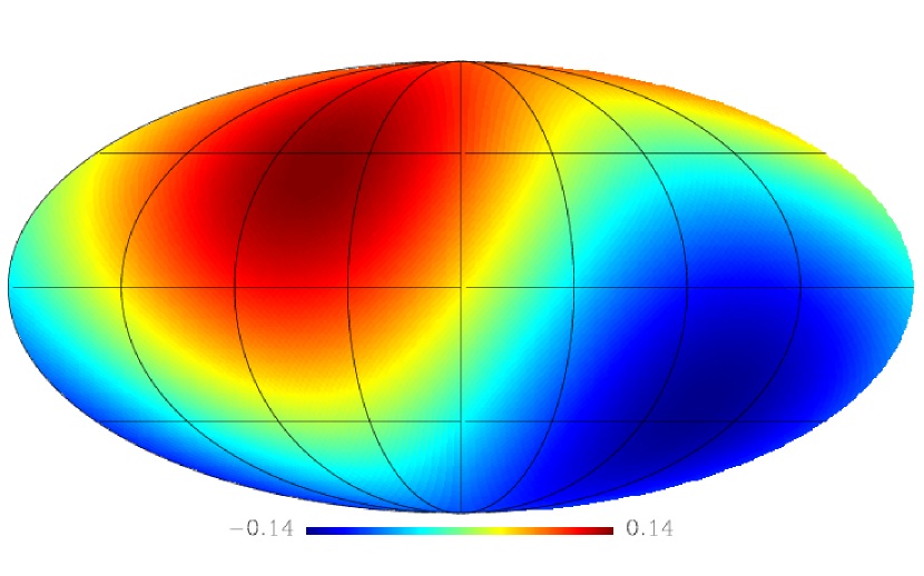
Figure 1: Maximum likelihood linear modulation function projected on the last scattering surface. High values indicate suppression of the primordial perturbations and low values indicate enhancement.

The marginalized distributions of $C_{2}$ to $C_{10}$ were found not to be significantly different from those in an unmodulated model (Hinshaw et al. 2006). The weight vector samples $(w_{x},w_{y},w_{z})$ were converted into Galactic co-latitude (varying between $0^{\circ},180^{\circ}$), longitude (varying between $-180^{\circ}$ and $180^{\circ}$) and percentage change of temperature variance in the direction of symmetry breaking $(\Delta\equiv 200(w_{x}^{2}+w_{y}^{2}+w_{z}^{2}))$. The two dimensional confidence intervals for the co-latitude and longitude are shown in LABEL:\ref{fig:results}.

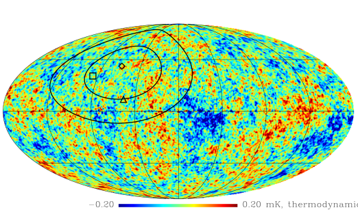
Figure 2: The contours enclosing 68% and 95% of the Monte Carlo samples. The maximum likelihood ($\diamond$) Galactic co-latitude and longitude is $(51^{\circ},68^{\circ})$. One of the most asymmetric directions found by Hansen et al. (2004a) ($\triangle$) is ($80^{\circ},57^{\circ}$). The north ecliptic ($\square$) is at ($60^{\circ},96^{\circ}$). This is plotted over the third year $N_{\rm side}=512$ ILC map (Hinshaw et al. 2006).

The marginalized one dimensional distributions are shown in LABEL:\ref{fig:pdfs}.

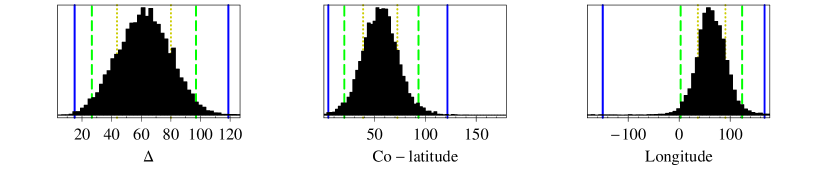
Figure 3: Marginalized distributions of the percentage change in the variance across the poles ($\Delta$) and the galactic coordinates of the direction of the modulation. The 68%, 95% and 99.7% confidence intervals are also shown.

Only $0.2\%$ of the samples were more than $90^{\circ}$ from the maximum likelihood point. The results are summarized in Table 1.

Table 1: Marginalized Statistics

Parameter	Mean	ML
$\Delta$	$62^{+18+35+57}_{-18-35-47}$	57
Colatitude	$56^{+17+36+65}_{-17-35-51}$	51
Longitude	$63^{+28+59+105}_{-26-58-213}$	68

5 Discussion and Conclusions

In this article the modulation model investigated by Spergel et al. (2006) has been extended by including a marginalization over the unmodulated monopole and dipole. This additional feature is required if the apparent isotropy breaking had a primordial origin. Including this marginalization improved the $\Delta\chi_{\rm eff}^{2}$ value from -3 to -9.

As seen from the confidence intervals in Table 1 and LABEL:\ref{fig:pdfs}, the marginalized posterior probability of $\Delta$ has its maximum more than three sigma away from the unmodulated case ($\Delta=0$). The modulated model is also preferred by the Akaike Information Criteria (AIC) (Akaike 1974; Magueijo & Sorkin 2006). It is not preferred by the Bayesian Information Criteria (BIC) (Schwarzy 1978; Magueijo & Sorkin 2006). However, the BIC is an approximation of the Bayesian evidence and assumes a prior for the parameters which is equivalent to one observation (Raftery 1995). The Bayesian evidence will be inversely proportional to the volume of the prior probability distribution of the modulation parameters. It may be hard to produce a modulation larger than one without effecting the observed dipole. A reevaluation of the Bayesian evidence is needed to see how it depends on the assumed prior. This could be done using a nested sampling algorithm (Mukherjee et al. 2006) which, unlike the BIC, does not require a Gaussian approximation to be made for the posterior distribution.

Spergel et al. (2006) also evaluated whether there was an additional quadrupolar component to the modulation. This component could potentially be useful in explaining the alignment and planarity of the quadrupole ($\ell=2$) and octopole ($\ell=3$) seen in the WMAP temperature data (de Oliveira-Costa et al. 2004; Schwarz et al. 2004). The normal direction of the plane of alignment is $(30^{\circ},-100^{\circ})$. Also, when the coordinate system is rotated in the direction of the normal of the $\ell=2,3$ planarity there is anomalous power in the $m=3$ component of the $\ell=5$ multipole (Land & Magueijo 2005b). Spergel et al. (2006) found that including a dipolar and quadrupolar component to the modulation improved $\Delta\chi_{\rm eff}^{2}$ by only 8 for a total of 8 extra parameters. Higher order terms in a spatial modulation could be implemented as terms quadratic in the spatial coordinates. Whether these additional terms will become significant when an unmodulated monopole and dipole are marginalized over will be part of a future investigation.

The effect of marginalization over foregrounds was checked and found not to play a big role. Similar improvements are obtained when the foreground corrected V band is used instead of marginalization. Also, the results are not sensitive to the exact method of degrading and applying the mask. A Kp2 extended mask (Eriksen et al. 2006) did not make a significant difference. Including additional $C_{\ell}$, with $\ell>10$, as parameters to be estimated (rather than set to their unmodulated ML values), also does not significantly effect the results.

It is interesting to compare the estimated modulation found in this article to that of Hansen et al. (2004a). The 10 most effective axes of symmetry breaking, for a range of scales, are plotted in their LABEL:24. A similar area, to the two dimensional confidence intervals in LABEL:\ref{fig:results}, is covered. Also, their LABEL:19 compares the power spectra in different hemispheres. The range of values is consistent with the confidence intervals for $\Delta$ in Table 1 and LABEL:\ref{fig:pdfs}.

Prunet et al. (2005) tested for a dipolar modulation. However, the largest scale they looked at was $\ell=20$ to 100 binned. They did not get significant results in that range. As the observed modulation only occurs for $\ell\lesssim 40$ (Hansen et al. 2004a), the $\ell=20$ to $100$ range would not be expected to show significant modulation when binned.

Freeman et al. (2006) propose that the modulation of $\ell=2$ to $\ell=7$ may be sensitive to any residual unmodulated dipole component. This is not a concern for the approach taken in this article as an unmodulated dipole is projected out of the likelihood, see Eq. (11).

Searches for lack of isotropy using a method based on a bipolar expansion of the two point correlation function do not detect the north south asymmetry in the $\ell=2$ to $\ell=40$ range (Hajian & Souradeep 2006; Armendariz-Picon 2006). The linear modulation model could be used to understand why the bipolar estimator is insensitive to this type of isotropy breaking.

A small scale cut off in the modulation implies that a linear modulation of the primordial power spectrum would only apply to wave numbers larger than about $4\times 10^{-3}h$ Mpc^-1. It would be interesting to evaluate whether this modulation would be detectable in future large scale galaxy surveys. However, at a redshift of one the change in the variance at opposite poles would only be about four percent, due to the smaller comoving distance.

A number of attempts have been made to explain the asymmetry in terms of local nonlinear inhomogeneities (Moffat 2005; Tomita 2005a, b; Inoue & Silk 2006). It would be interesting to see if the polarization maps of the CMB (Page et al. 2006) could be used to distinguish local effects from a modulation of the primordial perturbations.

Primordial magnetic fields (Durrer et al. 1998; Chen et al. 2004; Naselsky et al. 2004), global topology (de Oliveira-Costa et al. 2004; Kunz et al. 2006), and anisotropic expansion (Berera et al. 2004; Buniy et al. 2006; Gumrukcuoglu et al. 2006) can also lead to isotropy breaking. However, in these cases the modulating function is of higher order than dipolar and so these mechanisms are better suited for explaining the alignment between $\ell=2$ and $\ell=3$ and the high $(\ell,m)=(5,3)$ mode (Gordon et al. 2005).

An additive template based on a Bianchi $VII_{h}$ model has been shown to provide a good fit to the asymmetry (Jaffe et al. 2005). However, the model is only empirical as it would require a very open Universe which is in conflict with many other observations. It is harder for additive templates to explain the alignment between $\ell=2$ and $\ell=3$ as this requires a chance cancellation between an underlying Gaussian field and a deterministic template (Gordon et al. 2005; Land & Magueijo 2006).

As seen in LABEL:\ref{fig:results}, the maximum likelihood direction of modulation was found to be about $44^{\circ}$ from the ecliptic north pole. Only about 9% of the time would two randomly chosen directions be as close, or closer, together. This may be an indication that the modulation is caused by some systematic effect or foreground. However, as can be seen from LABEL:\ref{fig:results}, the confidence intervals, for the direction of modulation, cover just under half the northern hemisphere. Therefore, the actual direction, of modulation may be significantly further away from the ecliptic north pole.

Standard single field inflation would produce isotropic perturbations. However, multi-field models, such as in the curvaton scenario (Lyth & Wands 2002; Mollerach 1990; Linde & Mukhanov 1997; Enqvist & Sloth 2002; Moroi & Takahashi 2001), can produce, what to a particular observer appear to be, non-isotropic perturbations (Linde & Mukhanov 2006). The curvaton mechanism produces a web like structure in which relatively stable domains are separated by walls of large nonlinear fluctuations. If the mass of the curvaton field is sufficiently small, our observable Universe could be enclosed within a stable domain. If we happen to live near one of the walls, of a domain, then the amplitude of the perturbations will be larger on the side of the observed Universe closer to the wall (Linde & Mukhanov 2006). However, if our observed Universe was far enough away from the web walls, the very large scale fluctuations would be linear and so isotropy would be unlikely to appear to be broken (Lyth 2006). As the non-isotropic nature only extends to about $\ell=40$ (Hansen et al. 2004a), it would be necessary for the inflaton perturbations to dominate over the curvaton ones for wave numbers larger than about $4\times 10^{-3}h$ Mpc^-1. The curvaton produces curvature perturbations proportional to $V^{1/2}$ (Lyth & Wands 2002), where $V$ denotes the inflaton potential. While the inflaton produces curvature perturbations proportional to $V^{3/2}/V^{\prime}$, where $V^{\prime}$ denotes the slope of the potential. So if there is a sudden drop in $V$ and $V^{\prime}$, it is possible for the non-isotropic curvaton perturbations to dominate for wave numbers smaller than $4\times 10^{-3}h$ Mpc^-1 and inflaton perturbations to dominate for larger wave numbers.

There are oscillations in the WMAP power spectrum, at around $\ell=40$, which may be caused by a change of slope in the inflaton potential (Covi et al. 2006). Whether all these elements can be put together to make a working curvaton model, that fits the data as well as a linear modulation, is still being investigated.

The results presented here provide a parameterization for the observed asymmetry between different hemispheres of the WMAP data. Having a specific model for the primordial fluctuations will make it easier to develop new tests for this asymmetry and help determine if it is a genuine window into new physics at the largest observable scales.

References

- Akaike (1974) Akaike, H. 1974, IEEE Transactions on Automatic Control, 19, 716
- Armendariz-Picon (2006) Armendariz-Picon, C. 2006, Journal of Cosmology and Astro-Particle Physics, 3, 2
- Bardeen (1980) Bardeen, J. M. 1980, Phys. Rev. D, 22, 1882
- Bennett et al. (1996) Bennett, C. L., Banday, A. J., Gorski, K. M., Hinshaw, G., Jackson, P., Keegstra, P., Kogut, A., Smoot, G. F., Wilkinson, D. T., & Wright, E. L. 1996, ApJ, 464, L1+
- Bennett et al. (2003) Bennett, C. L., Halpern, M., Hinshaw, G., Jarosik, N., Kogut, A., Limon, M., Meyer, S. S., Page, L., Spergel, D. N., Tucker, G. S., Wollack, E., Wright, E. L., Barnes, C., Greason, M. R., Hill, R. S., Komatsu, E., Nolta, M. R., Odegard, N., Peiris, H. V., Verde, L., & Weiland, J. L. 2003, ApJS, 148, 1
- Berera et al. (2004) Berera, A., Buniy, R. V., & Kephart, T. W. 2004, Journal of Cosmology and Astro-Particle Physics, 10, 16
- Bernui et al. (2005) Bernui, A., Mota, B., Reboucas, M. J., & Tavakol, R. 2005, astro-ph/0511666
- Bernui et al. (2006) Bernui, A., Villela, T., Wuensche, C. A., Leonardi, R., & Ferreira, I. 2006, astro-ph/0601593
- Bond et al. (1998) Bond, J. R., Jaffe, A. H., & Knox, L. 1998, Phys. Rev. D, 57, 2117
- Buniy et al. (2006) Buniy, R. V., Berera, A., & Kephart, T. W. 2006, Phys. Rev. D, 73, 063529
- Chen et al. (2004) Chen, G., Mukherjee, P., Kahniashvili, T., Ratra, B., & Wang, Y. 2004, ApJ, 611, 655
- Copi et al. (2004) Copi, C. J., Huterer, D., & Starkman, G. D. 2004, Phys. Rev. D, 70, 043515
- Covi et al. (2006) Covi, L., Hamann, J., Melchiorri, A., Slosar, A., & Sorbera, I. 2006, astro-ph/0606452
- Cruz et al. (2005) Cruz, M., Martínez-González, E., Vielva, P., & Cayón, L. 2005, MNRAS, 356, 29
- de Oliveira-Costa et al. (2004) de Oliveira-Costa, A., Tegmark, M., Zaldarriaga, M., & Hamilton, A. 2004, Phys. Rev. D, 69, 063516
- Durrer et al. (1998) Durrer, R., Kahniashvili, T., & Yates, A. 1998, Phys. Rev. D, 58, 123004
- Enqvist & Sloth (2002) Enqvist, K. & Sloth, M. S. 2002, Nuclear Physics B, 626, 395
- Eriksen et al. (2004) Eriksen, H. K., Hansen, F. K., Banday, A. J., Górski, K. M., & Lilje, P. B. 2004, ApJ, 609, 1198
- Eriksen et al. (2006) Eriksen, H. K., Huey, G., Saha, R., Hansen, F. K., Dick, J., Banday, A. J., Gorski, K. M., Jain, P., Jewell, J. B., Knox, L., Larson, D. L., O’Dwyer, I. J., Souradeep, T., & Wandelt, B. D. 2006, astro-ph/0606088
- Freeman et al. (2006) Freeman, P. E., Genovese, C. R., Miller, C. J., Nichol, R. C., & Wasserman, L. 2006, ApJ, 638, 1
- Gordon et al. (2005) Gordon, C., Hu, W., Huterer, D., & Crawford, T. 2005, Phys. Rev. D, 72, 103002
- Górski et al. (2005) Górski, K. M., Hivon, E., Banday, A. J., Wandelt, B. D., Hansen, F. K., Reinecke, M., & Bartelmann, M. 2005, ApJ, 622, 759
- Gumrukcuoglu et al. (2006) Gumrukcuoglu, A. E., Contaldi, C. R., & Peloso, M. 2006, astro-ph/0608405
- Hajian & Souradeep (2006) Hajian, A. & Souradeep, T. 2006, astro-ph/0607153
- Hansen (2004) Hansen, F. K. 2004, astro-ph/0406393
- Hansen et al. (2004a) Hansen, F. K., Banday, A. J., & Górski, K. M. 2004a, MNRAS, 354, 641
- Hansen et al. (2004b) Hansen, F. K., Cabella, P., Marinucci, D., & Vittorio, N. 2004b, ApJ, 607, L67
- Hinshaw et al. (2006) Hinshaw, G., Nolta, M. R., Bennett, C. L., Bean, R., Dore’, O., Greason, M. R., Halpern, M., Hill, R. S., Jarosik, N., Kogut, A., Komatsu, E., Limon, M., Odegard, N., Meyer, S. S., Page, L., Peiris, H. V., Spergel, D. N., Tucker, G. S., Verde, L., Weiland, J. L., Wollack, E., & Wright, E. L. 2006, astro-ph/0603451
- Hu & Sugiyama (1995) Hu, W. & Sugiyama, N. 1995, ApJ, 444, 489
- Inoue & Silk (2006) Inoue, K. T. & Silk, J. 2006, ArXiv Astrophysics e-prints
- Jaffe et al. (2005) Jaffe, T. R., Banday, A. J., Eriksen, H. K., Górski, K. M., & Hansen, F. K. 2005, ApJ, 629, L1
- Jarosik et al. (2006) Jarosik, N., Barnes, C., Greason, M. R., Hill, R. S., Nolta, M. R., Odegard, N., Weiland, J. L., Bean, R., Bennett, C. L., Dore’, O., Halpern, M., Hinshaw, G., Kogut, A., Komatsu, E., Limon, M., Meyer, S. S., Page, L., Spergel, D. N., Tucker, G. S., Wollack, E., & Wright, E. L. 2006, astro-ph/0603452
- Kunz et al. (2006) Kunz, M., Aghanim, N., Cayon, L., Forni, O., Riazuelo, A., & Uzan, J. P. 2006, Phys. Rev. D, 73, 023511
- Land & Magueijo (2005a) Land, K. & Magueijo, J. 2005a, MNRAS, 357, 994
- Land & Magueijo (2005b) —. 2005b, Physical Review Letters, 95, 071301
- Land & Magueijo (2006) —. 2006, MNRAS, 367, 1714
- Larson & Wandelt (2004) Larson, D. L. & Wandelt, B. D. 2004, ApJ, 613, L85
- Linde & Mukhanov (1997) Linde, A. & Mukhanov, V. 1997, Phys. Rev. D, 56, 535
- Linde & Mukhanov (2006) —. 2006, Journal of Cosmology and Astro-Particle Physics, 4, 9
- Lyth (2006) Lyth, D. H. 2006, Journal of Cosmology and Astro-Particle Physics, 6, 15
- Lyth & Wands (2002) Lyth, D. H. & Wands, D. 2002, Physics Letters B, 524, 5
- Magueijo & Sorkin (2006) Magueijo, J. & Sorkin, R. D. 2006, astro-ph/0604410
- Moffat (2005) Moffat, J. W. 2005, Journal of Cosmology and Astro-Particle Physics, 10, 12
- Mollerach (1990) Mollerach, S. 1990, Phys. Rev. D, 42, 313
- Moroi & Takahashi (2001) Moroi, T. & Takahashi, T. 2001, Physics Letters B, 522, 215
- Mukherjee et al. (2006) Mukherjee, P., Parkinson, D., & Liddle, A. R. 2006, ApJ, 638, L51
- Naselsky et al. (2004) Naselsky, P. D., Chiang, L.-Y., Olesen, P., & Verkhodanov, O. V. 2004, ApJ, 615, 45
- Page et al. (2006) Page, L., Hinshaw, G., Komatsu, E., Nolta, M. R., Spergel, D. N., Bennett, C. L., Barnes, C., Bean, R., Dore’, O., Halpern, M., Hill, R. S., Jarosik, N., Kogut, A., Limon, M., Meyer, S. S., Odegard, N., Peiris, H. V., Tucker, G. S., Verde, L., Weiland, J. L., Wollack, E., & Wright, E. L. 2006, astro-ph/0603450
- Park (2004) Park, C.-G. 2004, MNRAS, 349, 313
- Prunet et al. (2005) Prunet, S., Uzan, J.-P., Bernardeau, F., & Brunier, T. 2005, Phys. Rev. D, 71, 083508
- Raftery (1995) Raftery, A. 1995, Sociological Methodology, 25, 111
- Sachs & Wolfe (1967) Sachs, R. K. & Wolfe, A. M. 1967, ApJ, 147, 73
- Schwarz et al. (2004) Schwarz, D. J., Starkman, G. D., Huterer, D., & Copi, C. J. 2004, Physical Review Letters, 93, 221301
- Schwarzy (1978) Schwarzy, G. 1978, Annals of Statistics, 6, 461
- Slosar & Seljak (2004) Slosar, A. & Seljak, U. 2004, Phys. Rev. D, 70, 083002
- Slosar et al. (2004) Slosar, A., Seljak, U., & Makarov, A. 2004, Phys. Rev. D, 69, 123003
- Spergel et al. (2006) Spergel, D. N., Bean, R., Dore’, O., Nolta, M. R., Bennett, C. L., Hinshaw, G., Jarosik, N., Komatsu, E., Page, L., Peiris, H. V., Verde, L., Barnes, C., Halpern, M., Hill, R. S., Kogut, A., Limon, M., Meyer, S. S., Odegard, N., Tucker, G. S., Weiland, J. L., Wollack, E., & Wright, E. L. 2006, astro-ph/0603449
- Tegmark et al. (1998) Tegmark, M., Hamilton, A. J. S., Strauss, M. A., Vogeley, M. S., & Szalay, A. S. 1998, ApJ, 499, 555
- Tomita (2005a) Tomita, K. 2005a, Phys. Rev. D, 72, 103506
- Tomita (2005b) —. 2005b, Phys. Rev. D, 72, 043526
- Vielva et al. (2004) Vielva, P., Martínez-González, E., Barreiro, R. B., Sanz, J. L., & Cayón, L. 2004, ApJ, 609, 22
- Wright et al. (1992) Wright, E. L., Meyer, S. S., Bennett, C. L., Boggess, N. W., Cheng, E. S., Hauser, M. G., Kogut, A., Lineweaver, C., Mather, J. C., Smoot, G. F., Weiss, R., Gulkis, S., Hinshaw, G., Janssen, M., Kelsall, T., Lubin, P. M., Moseley, Jr., S. H., Murdock, T. L., Shafer, R. A., Silverberg, R. F., & Wilkinson, D. T. 1992, ApJ, 396, L13