Isotherms clustering in cosmic microwave background

Abstract

Isotherms clustering in cosmic microwave background (CMB) has been studied using the 3-year WMAP data on cosmic microwave background radiation. It is shown that the isotherms clustering could be produced by the baryon-photon fluid turbulence in the last scattering surface. The Taylor-microscale Reynolds number of the turbulence is estimated directly from the CMB data as $Re_{\lambda}\sim 10^{2}$.

I Introduction

Luminous matter in the observable universe is strongly clustered (see, for a review p1 ). Main reasons for this apparent clustering are gravitational forces and an initial non-uniformity of the baryon-photon matter just before the recombination time. An information about this non-uniformity we can infer from the Cosmic Microwave Background (CMB) radiation maps. Although these maps indicate nearly Gaussian distribution of the CMB fluctuations, certain clustering may be observed already in these maps even after they have monopole and dipole set to zero. The clustering of the isotherms in the last scattering surface then can be used as an initial condition for the gravitational simulations. One of the purposes of this paper is to describe the clustering quantitatively. Another related purpose is to find out underlying primordial physical processes, which may cause the isotherms clustering in the CMB maps. It is known sbar ,dky that rotational velocity perturbations in the primordial baryon-photon fluid can produce angular scale anisotropies in CMB radiation through the Doppler effect. The conclusions are relevant to arcminute scales (for large scales see jaf ). On the other hand, it is recently shown in sb1 that clustering is an intrinsic property of the turbulent (rotational) velocity field. Therefore, one should check whether the CMB isotherms clustering can be related to turbulent motion of the baryon-photon fluid just before recombination time (an observational indication of turbulent motion in the baryon-photon fluid just before recombination time is given in bs1 , see also gibson -kah ). Moreover, we will estimate the Taylor-microscale Reynolds number ($Re_{\lambda}$, see Appendix A) of this motion, that is $Re_{\lambda}\sim 10^{2}$ (let us recall that critical value is $Re_{\lambda}\simeq 40$ ). As far as we know this is first estimate of the Reynolds number obtained directly from a CMB-map (we have used a cleaned 3-year WMAP tag ).

To find physical (dynamical) origin of the isotherms clustering in the CMB we will compare certain statistical properties of the CMB maps (and their Gaussian simulations) with corresponding properties of the fluid turbulence. It is well known that energetically the CMB fluctuations are dominated by acoustic perturbations of the primordial velocity field. The velocity field can be represented by following way

$${\bf u}={\bf u_{a}}+{\bf u_{r}}$$

where the acoustic component is a potential one ${\bf u_{a}}=\nabla\varphi$ and ${\bf u_{r}}$ is rotational component of the primordial velocity field. To exclude the acoustic component one can take operation $curl~{}{\bf u}=curl~{}{\bf u_{r}}$, that is vorticity. Average energy dissipation in turbulent velocity field is determined just by its rotational component my

$$\langle\varepsilon\rangle\sim\nu\langle(curl~{}{\bf u})^{2}\rangle$$

where $\langle...\rangle$ means statistical average and $\nu$ is kinematic viscosity. Since it is expected that high frequency events in the velocity field should provide the most significant contribution to the turbulent dissipation and, especially, to its high order moments one can also expect that clustering in turbulent velocity field should be intimately related to fluctuations of the energy dissipation (so-called intermittency phenomenon my ,sa ). Taking into account that turbulent velocity is nearly Gaussian my (see also Appendix B) the clustering phenomenon in the turbulent velocity field should be also a Gaussian one. On the other hand, the intermittency phenomenon in fluid turbulence, usually associated with fine non-Gaussian properties of the velocity field my ,sa . Thus, simultaneous consideration of the cluster and intermittency characteristics can provide an additional valuable information about physical origin of the isotherms clustering in the CMB maps and about the fine non-Gaussianity of the maps. Therefore, the paper starts with an introduction to this subject.

II Clustering and intermittency

For turbulent flows the so-called Taylor hypothesis is generally used to interpret the turbulent data my ,sa ,b . This hypothesis states that the intrinsic time dependence of the wavefields can be ignored when the turbulence is convected past the probes at nearly constant speed. With this hypothesis, the temporal dynamics should reflect the spatial one, i.e. the fluctuating velocity field measured by a given probe as a function of time, $u(t)$ is the same as the velocity $u(x/\langle u\rangle)$ where $\langle u\rangle$ is the mean velocity and $x$ is the distance to a position ”upstream” where the velocity is measured at $t=0$.

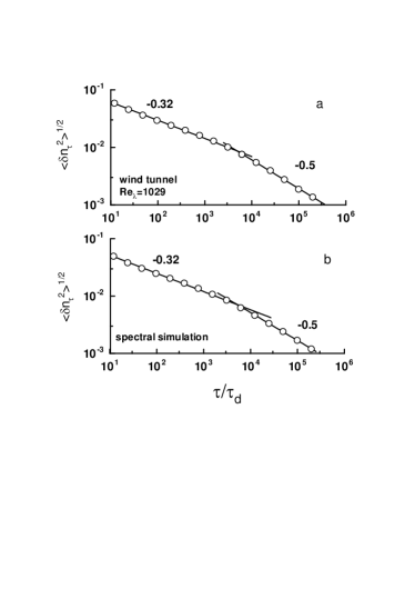
Figure 1: Standard deviation of the running density fluctuations against $\tau$ for for the velocity fluctuations measured in the wind-tunnel (Fig. 1a) and for their Gaussian spectral simulation (Fig. 1b).

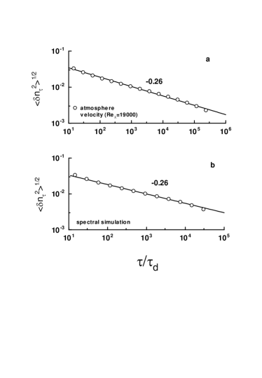
Figure 2: As in Fig. 1 but for atmospheric surface layer at $Re_{\lambda}=19000$ (Fig. 2a) and for its Gaussian spectral simulation (Fig. 2b).

Let us count the number of ’zero’-crossing points of the signal in a time interval $\tau$ and consider their running density $n_{\tau}$. Let us denote fluctuations of the running density as $\delta n_{\tau}=n_{\tau}-\langle n_{\tau}\rangle$, where the brackets mean the average over long times. We are interested in scaling variation of the standard deviation of the running density fluctuations $\langle\delta n_{\tau}^{2}\rangle^{1/2}$ with $\tau$

$$\langle\delta n_{\tau}^{2}\rangle^{1/2}\sim\tau^{-\alpha_{n}}$$

For white noise it can be derived analytically molchan ,lg that $\alpha_{n}=1/2$ (see also sb1 ).

In Figure 1a and 2a we show calculations of the standard deviation for a turbulent velocity signal obtained in the wind-tunnel experiment pkw and for a velocity signal obtained in an atmospheric experiment sd ) respectively. The straight lines are drawn in the figures to indicate scaling (1). One can see two scaling intervals in Fig. 1a. The left scaling interval covers both dissipative and inertial ranges, while the right scaling interval covers scales larger then the integral scale of the flow. While the right scaling interval is rather trivial (with $\alpha_{n}=1/2$, i.e. without clustering), the scaling in the left interval (with $\alpha_{n}<1/2$) indicates clustering of the high frequency fluctuations. The cluster-exponent $\alpha_{n}$ decreases with increase of $Re_{\lambda}$, that means increasing of the clustering (as it was expected from qualitative observations).

To describe intermittency the standard deviation of fluctuations of the energy dissipation is used po (see also a discussion in lp )

$$\langle\delta\varepsilon_{\tau}^{2}\rangle^{1/2}\sim\tau^{-\alpha_{i}}$$

where

$$\varepsilon_{\tau}=\frac{\int_{0}^{\tau}\varepsilon(t)dt}{\tau},$$

or in the terms of the discrete time series sa

$$\varepsilon_{\tau}\sim\sum_{j=1}^{\tau}\Delta u_{j}^{2}/\tau$$

where $\Delta u_{j}=u_{j+1}-u_{j}$.

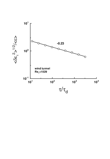
Figure 3: Intermittency exponent as slope of the straight line for the longitudinal velocity signal obtained in the wind tunnel experiment pkw at $Re_{\lambda}=1029$.

Figure 3 shows an example of the scaling (2) providing the intermittency exponent $\alpha_{i}$ for the wind-tunnel data (see po for more details).

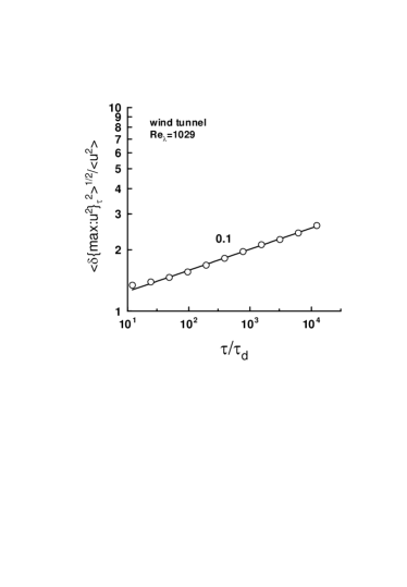
Figure 4: Statistical (’tail’) exponent $\alpha_{m}\simeq 0.1$ as slope of the straight line for the velocity signal obtained in the wind tunnel experiment pkw at $Re_{\lambda}=1029$.

Events with high concentration of the zero-crossing points in the intermittent turbulent velocity signal provide main contribution to the $\langle\delta\varepsilon_{\tau}^{2}\rangle$ due to high concentration of the statistically significant local maximums in these events bt . Therefore, one can make use of statistical version of the theorem ’about mean’ in order to estimate the standard deviation

$$\langle\delta\varepsilon_{\tau}^{2}\rangle^{1/2}\sim\langle\delta\{\max:u^{2}\}_{\tau}^{2}\rangle^{1/2}\langle\delta n_{\tau}^{2}\rangle^{1/2}$$

where $\{\max:u^{2}\}_{\tau}$ is maximum of $u(t)^{2}$ in interval of length $\tau$. Value of $\langle\delta\{\max:u^{2}\}_{\tau}^{2}\rangle^{1/2}$ should grow with $Re_{\lambda}$ (due to increasing of $\langle u^{2}\rangle$) and, statistically, with the length of interval $\tau$ (the later growth is expected to be self-similar), i.e.

$$\langle\delta\{\max:u^{2}\}_{\tau}^{2}\rangle^{1/2}=C(Re_{\lambda})\cdot\tau^{\alpha_{m}}$$

where constant $C(Re_{\lambda})$ is a monotonically increasing function of $Re_{\lambda}$, and the statistical (’tail’) exponent $\alpha_{m}\geq 0$ is independent on $Re_{\lambda}$. Fig. 4 shows an example of scaling (5) providing the statistical (’tail’) exponent $\alpha_{m}\simeq 0.10\pm 0.01$ for the wind-tunnel data. Substituting (5) into (4) and taking into account (1) and (2) we can infer a relation between the scaling exponents

$$\alpha_{i}=\alpha_{n}-\alpha_{m}$$

Unlike the exponent $\alpha_{m}$ the exponent $\alpha_{n}$ depends on $Re_{\lambda}$. Therefore, we can learn from (6) that just the clustering of high frequency velocity fluctuations ($\alpha_{n}$ in (6)) is responsible for dependence of the intermittency exponent $\alpha_{i}$ on the $Re_{\lambda}$.

It is naturally consider the exponent functions through $\ln R_{\lambda}$: $\alpha=\alpha(\ln Re_{\lambda})$ sb1 ,cgh ,bg (see also Appendix A). Following to the general idea of Ref. bg (see also sb1 ) let us expend this function for large $Re_{\lambda}$ in a power series:

$$\alpha(\ln Re_{\lambda})=\alpha(\infty)+\frac{a_{1}}{\ln Re_{\lambda}}+\frac{a_{2}}{(\ln Re_{\lambda})^{2}}+...$$

In Figure 5 we show the calculated values of $\alpha_{n}$ (circles) and $\alpha_{i}$ (squares) for velocity signals against $1/\ln Re_{\lambda}$ for $200<Re_{\lambda}<20000$ (for $\alpha_{i}$ we also added four data points taken from the paper po , where the data were obtained in a mixing layer and in an atmospheric surface layer). The straight lines (the best fit) indicate approximation with the two first terms of the power series expansion

$$\alpha_{n}(\ln Re_{\lambda})\simeq 0.1+\frac{3/2}{\ln Re_{\lambda}},~{}~{}~{}~{}~{}~{}~{}~{}\alpha_{i}(\ln Re_{\lambda})\simeq\frac{3/2}{\ln Re_{\lambda}}$$

This means, in particular, that

$$\lim_{Re_{\lambda}\rightarrow\infty}\alpha_{n}\simeq 0.1,~{}~{}~{}~{}~{}\lim_{Re_{\lambda}\rightarrow\infty}\alpha_{i}\simeq 0$$

The closeness of the constants $a_{1}\simeq 3/2$ (the slopes of the straight lines in Fig. 5) in the approximations (8) of the cluster-exponent $\alpha_{n}$ and of the intermittency exponent $\alpha_{i}$ confirms the relationship (6) with $\alpha_{m}\simeq 0.1$ (cf. Figs. 4 and 5).

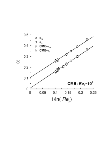
Figure 5: The cluster-exponent $\alpha_{n}$ (circles) and intermittency exponent $\alpha_{i}$ (squares) against $1/\ln Re_{\lambda}$ for velocity signals at different values of Reynolds number ($200<Re_{\lambda}<20000$).

Thus one can see from Eq. (6) that entire dependence of the intermittency exponent $\alpha_{i}$ on $Re_{\lambda}$ is determined by dependence of the cluster-exponent $\alpha_{n}$ on $Re_{\lambda}$. On the other hand, the cluster-exponent itself is uniquely determined by energy spectrum of the velocity signal at suggestion that the velocity field is Gaussian. However, different spectra can produce the same value of the cluster-exponent (in particular, the cluster-exponent is invariant to variation of the potential component of the velocity field, that is significant for next section).

We use spectral simulation to illustrate that energy spectrum uniquely determines cluster-exponent for Gaussian-like turbulent signals. In these simulations we generate Gaussian stochastic signal with energy spectrum given as data (the spectral data are taken from the original velocity signals). Figures 1b and 2b show, as examples, results of such simulation for the wind-tunnel velocity data (Fig. 1b) and for the atmospheric surface layer (Fig. 2b). Namely, Figures 1a and 2a show results of calculations for the original velocity signals and Figs. 1b, and 2b show corresponding results obtained for the spectral simulations of the signals. This means, in particular, that in respect to the cluster-exponent the turbulent velocity signals exhibit Gaussian properties. Of course, it is not the case for the intermittency exponent $\alpha_{i}$. Namely, $\alpha_{i}\simeq 0.5$ for the Gaussian spectral simulations, independently on the spectral shape.

III CMB clustering and intermittency

The motion of the scatterers in the last scattering surface imprints a temperature fluctuation, $\Delta T$, on the CMB through the Doppler effect sbar ,dky

$$\frac{\Delta T({\bf n})}{T}\sim\int g(L){\bf n}\cdot{\bf v_{b}}({\bf x})~{}dL$$

where ${\bf n}$ is the direction (the unit vector) on the sky, ${\bf v_{b}}$ is the velocity field of the baryons evaluated along the line of sight, ${\bf x}=L{\bf n}$, and $g$ is the so-called visibility. It should be noted that, in a potential flow, fluctuations perpendicular to the line of sight lack a velocity component parallel to the line of sight; consequently, generally there is no Doppler effect for the potential flows. The same is not true for rotational flows, since the waves that run perpendicular to the line of sight have velocities parallel to the line of site ov .

Clustering in the turbulent velocity field in the last scattering surface, therefore, can produce clustering of the observed CMB isotherms. Thus (see previous section), the areas of strong clustering of the CMB isotherms can indicate the areas of the strong vorticity activity in last scattering surface. Moreover, using results of previous section we can, calculating corresponding cluster- and intermittency exponents for the CMB maps, check whether the turbulent relationship (6) is also valid for the CMB data, with the same value of $\alpha_{m}\simeq 0.1$ as for the fluid turbulence. In the case of positive answer we can then estimate the Taylor-microscale Reynolds number $Re_{\lambda}$ for the primordial turbulence in the last scattering surface using Fig. 5.

We used the 3-year WMAP data cleaned from foreground contamination by Tegmark’s group tag (the original temperature is given in $\mu K$ units). Let us introduce a gradient measure for the cosmic microwave radiation temperature $T$ fluctuations that is an analogy of the turbulent energy dissipation measure $\varepsilon_{r}$ sa ,b

$$\chi_{r}=\frac{\int_{v_{r}}(\bigtriangledown{T})^{2}dv}{v_{r}}$$

where $v_{r}$ is a subvolume with space-scale $r$ (this is a space analogy of Eqs. (3a,b), see also Introduction: $\langle\varepsilon\rangle\sim\langle(curl~{}{\bf v})^{2}\rangle$).

Then, scaling law

$$\langle\delta\chi_{r}^{2}\rangle\sim r^{-\alpha_{i}}$$

corresponds to the scaling law (2) and the exponent $\alpha_{i}$ is the CMB intermittency exponent. Technically, using the cosmic microwave pixel data map, we will calculate the cosmic microwave radiation temperature gradient measure using summation over pixel sets (by random walks method) instead of integration over subvolumes $v_{r}$. The scaling of type (11) (if exists) will be then written as

$$\langle\delta\chi_{s}^{2}\rangle^{1/2}\sim s^{-\alpha_{i}}$$

where the metric scale $r$ is replaced by number of the pixels, $s$, characterizing the size of the summation set (the random walk trajectory length). The $\chi_{s}$ is a surrogate of the real 3D gradient measure $\chi_{r}$. It is believed that such surrogates can reproduce quantitative scaling properties of the 3D prototypes sa . Analogously to the previous section the cluster analysis can be performed

$$\langle\delta n_{s}^{2}\rangle^{1/2}\sim s^{-\alpha_{n}}$$

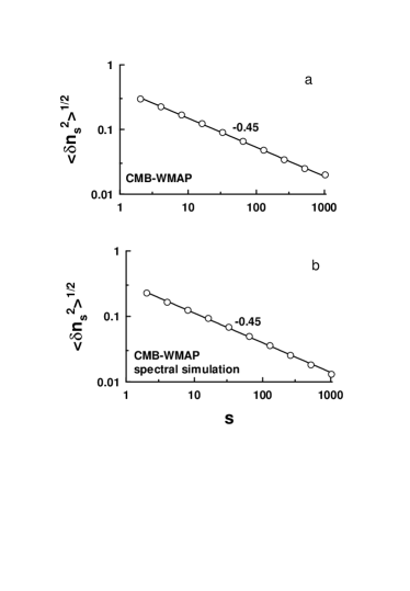
Figure 6: As in Figs. 1,2 but for the CMB fluctuations in the 3 year WMAP (Fig. 6a) and for the corresponding Gaussian spectral simulation map (Fig. 6b).

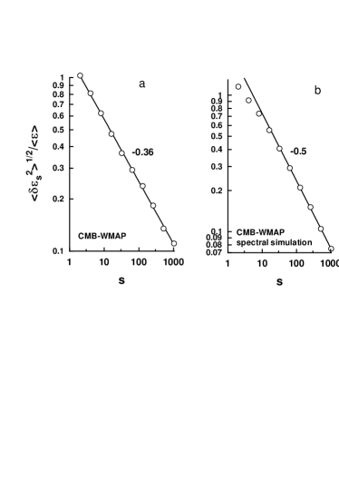
Figure 7: As in Fig. 3 but for the CMB fluctuations in the 3 year WMAP (Fig. 7a) and for the corresponding Gaussian spectral simulation map (Fig. 7b).

Figure 6a shows the cluster-scaling (13) for the CMB calculated for the 3-year WMAP map cleaned by Tegmark’s group tag . The straight line (the best fit) is drawn to indicate the scaling in log-log scales. Figure 6b shows the results of analogous calculations produced for Gaussian spectral simulation of the 3-year WMAP map. As it was expected the Gaussian spectral simulation produces map with the same cluster properties as the original map (cf. previous section).

The intermittency exponent $\alpha_{i}$, on the contrary, takes significantly different values for the original CMB map and for its Gaussian spectral simulation (Figs. (7a,b)). One can see, that for the Gaussian map-simulation $\alpha_{i}\simeq 0.5\pm 0.02$ (as it is expected, see previous section), while for the original CMB map $\alpha_{i}\simeq 0.36\pm 0.02$ in agreement with the fluid turbulence case (Eq. (6) and Fig. 5). Then, using Fig. 5 we can estimate the Taylor-microscale Reynolds number of the primordial turbulence in the last scattering surface (with logarithmic accuracy) $Re_{\lambda}\sim 10^{2}$.

It should be noted, that critical value (for transition from laminar to turbulent motion) is $Re_{\lambda}\simeq 40$ sb1 . Therefore, one can conclude that motion of the baryon-photon fluid at the recombination time is rather close to the critical state. This can be considered as an indication that the recombination process itself might be a source of the turbulence, which modulates the CMB. Indeed, the strong photon viscosity is known as the main reason for presumably laminar motion of the baryon-photon fluid just before recombination time. Therefore, if the recombination starts from appearance of the small localized transparent spots, then activity related to these spots can result in turbulent motion of the entire bulk of the baryon-photon fluid at the recombination time.

I thank K.R. Sreenivasan for inspiring cooperation. I also thank D. Donzis, C.H. Gibson and participants of the workshop ”Nonlinear cosmology: turbulence and fields” for discussions.

Thin vortex tubes (or filaments) are the most prominent hydrodynamical elements of turbulent flows batchelor . The filaments are unstable in 3-dimensional space. In particular, a straight line-vortex can readily develop a kink propagating along the filament with a constant speed. To estimate the velocity of propagation of such a kink let us first recall the properties of a ring vortex batchelor . Its speed $v$ is related to its diameter $\lambda$ and strength $\Gamma$ through

$$v=\frac{\Gamma}{2\pi\lambda}\ln\left(\frac{\lambda}{2\eta}\right),$$

where $\eta$ is the radius of the core of the ring and $\lambda/2\eta\gg 1$ (see figure 8).

If, for instance, a straight line-vortex develops a kink with a radius of curvature $\lambda/2$, then self-induction generates a velocity perpendicular to the plane of the kink. This velocity can be also calculated using (A.1).

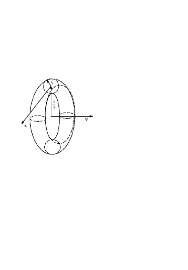
Figure 8: The vortex ring and its velocity.

One can guess that in a turbulent environment, the most unstable mode of a vortex tube with a thin core of length $L$ (integral scale) and radius $\eta$ (Kolmogorov or viscous scale), will be of the order $\lambda$: Taylor-microscale my . Then, the characteristic scale of velocity of the mode with the space scale $\lambda$ can be estimated with help of equation (A.1). Noting that the Taylor-microscale Reynolds number is defined as my

$$Re_{\lambda}=\frac{v_{0}\lambda}{\nu},$$

where $v_{0}$ is the root-mean-square value of a component of velocity. It is clear that the velocity that is more relevant (at least for the processes related to the vortex instabilities) for the space scale $\lambda$ is not $v_{0}$ but $v$ given by (A.1). Therefore, corresponding effective Reynolds number should be obtained by the renormalization of the characteristic velocity in (A.2) sb1 , as

$$Re_{\lambda}^{eff}=\frac{v\lambda}{\nu}\sim\frac{\Gamma}{2\pi\nu}\ln\left(\frac{\lambda}{2\eta}\right).$$

It can be readily shown from the definition that

$$\frac{\lambda}{\eta}=const~{}Re_{\lambda}^{1/2}$$

where $const=15^{1/4}\simeq 2$. Hence

$$Re_{\lambda}^{eff}\sim\frac{\Gamma}{4\pi\nu}\ln(Re_{\lambda})$$

The strength $\Gamma$ can be estimated as

$$\Gamma\sim 2\pi v_{\eta}\eta$$

where $v_{\eta}=\nu/\eta$ is the velocity scale for the Kolmogorov (or viscous) space scale $\eta$ my . Substituting (A.6) into (A.5) we obtain

$$Re_{\lambda}^{eff}\sim\ln(Re_{\lambda}).$$

Thus, for turbulence processes determined by the vortex instabilities the relevant dimensionless characteristic is $\ln(Re_{\lambda})$ rather than $Re_{\lambda}$ (cf Eq. (7) and Fig. 5).

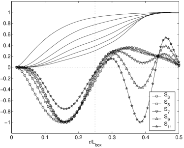
Figure 9: Moments $S_{p}$ versus $r/L_{box}$ obtained in a direct numerical simulation of fluid turbulence on a $2\pi$ cube at $128^{3}$ resolution $Re_{\lambda}\approx 55$ d . Upper curves correspond to $p=2,4,6,8,10,12$, the curves with symbols correspond to $p=1,3,5,7,9,11$. For $r/L_{box}\geq 0.5$ the picture is a mirror reflection of that shown in the figure.

In this Appendix we will show that modulation of the CMB by the primordial turbulence at the last scattering surface can exhibit Gaussian properties much more strong than those of the ’normal’ fluid turbulence, while preserving the turbulence properties intact.

We always observe the CMB photons emitted from the ’boundary’ (the last scattering surface). Therefore, definition of the ’boundary conditions’ for the dynamic universe is crucial in the case of the CMB radiation. Naturally this is a very non-trivial task to define boundary conditions for the universe (horizon). In the numerical simulations of the homogeneous turbulence dynamics the periodic boundary conditions are often used. The periodic boundary conditions seem to be also a natural suggestion for the universe.

When one considers modulation of the CMB radiation by the Doppler effect only the relative difference in velocity between the observer and the source, separated by a distance $r$ along the line of sight: $\Delta u_{r}=u(x+r)-u(x)$, needs to be considered. Let us consider the moments of the velocity difference:

$$S_{p}(r)=\langle[u(x)-u(x+r)]^{p}\rangle$$

As an example, Fig. 9 shows results of a direct numerical simulation d of fluid turbulence with the periodical boundary conditions on a $2\pi$ cube (size $L_{box}$) at $128^{3}$ resolution $Re_{\lambda}\approx 55$. The curves in the upper part of the figure correspond to the even-order moments (B.1), while the curves with symbols correspond to the odd-order moments. For $r/L_{box}>0.5$ the picture is a mirror reflection of that shown in the Fig. 9. One can see that the Gaussian conditions: $S_{p}=0$, for the odd-order moments are satisfied at the observer point $r/L_{box}=0.5$. Actually, this is a direct consequence of the mirror symmetry provided by the periodic boundary conditions. Using the dynamical equations of the baryon-photon fluid it can be shown that the even-order moments are also consistent with the Gaussian conditions at the observer point $r/L_{box}=0.5$.

References

- (1) F. Sylos Labini, M. Montuori and L. Pietronero, Phys. Rep., 293 61 (1998)
- (2) K. Subramanian and J.D. Barrow. Phys. Rev. D, 58, 083502 (1998).
- (3) R. Durrer, T. Kahniashvili, and A. Yates, Phys. Rev. D, 58, 123004 (1998).
- (4) T.R. Jaffe, A.J. Banday, H.K. Eriksen, K.M. Gorski, F.K. Hansen, ApJ, 629, L1 (2005).
- (5) K.R. Sreenivasan and A. Bershadskii, J. Fluid Mech., 54 477 (2006).
- (6) A. Bershadskii and K.R. Sreenivasan, Phys. Lett. A, 299, 149 (2002).
- (7) C.H. Gibson, Appl., Scien. Res., 72, 161, (2004).
- (8) A. Brandenburg, Astrophys. J., 550, 824 (2001).
- (9) E. Vishniac and J. Cho, Astrophys. J., 550, 752 (2001).
- (10) A. Dolgov and D. Grasso, Phys. Rev. Lett., 88, 011301 (2002).
- (11) N. Kleeorin, D. Moss, I. Rogachevskii, and D. Sokoloff, A&A, 400, 9 (2003).
- (12) E. Vishniac, A. Lazarian, and J. Cho, Lect. Notes Phys. 614, 376 (2003).
- (13) K. Subramanian, A. Shukurov, and N.E.L Haugen, MNRAS 366, 1437 (2005).
- (14) T. Kahniashvili, astro-ph/0605440 (2006).
- (15) M. Tegmark, A. de Oliveira-Costa, A. Hamilton, Phys. Rev. D, 68, 123523 (2003) (http://space.mit.edu/home/tegmark/wmap.html).
- (16) Monin A. S. and Yaglom A.M., 1975 Statistical Fluid Mechanics: Mechanics of Turbulence, V. 2 (The MIT Press, Cambridge).
- (17) K.R. Sreenivasan and R.A. Antonia, Annu. Rev. Fluid Mech, 29, 435 (1997).
- (18) A. Bershadskii, Phys. Rev. Lett., 90, 041101 (2003).
- (19) G. Molchan, private communication.
- (20) M.R. Leadbetter and J.D. Gryer, Bull. Amer. Math. Soc. 71, 561 (1965).
- (21) B.R. Pearson, P.-A. Krogstad and W. van de Water, Phys. Fluids, 14, 1288 (2002).
- (22) K.R. Sreenivasan and B. Dhruva, Prog. Theor. Phys. Suppl., 130, 103 (1998).
- (23) A. Praskovsky and S. Oncley, Fluid Dyn. Res. 21, 331 (1997).
- (24) V.S. L’vov and I. Procaccia, Phys. Rev. Lett., 74, 2690 (1995).
- (25) A. Bershadskii and A. Tsinober, Phys. Lett. A, 165, 37 (1992).
- (26) B. Castaing, Y. Gagne and E.J. Hopfinger, Physica D, 46, 177 (1990).
- (27) G.I. Barenblatt and N. Goldenfeld, Phys. Fluids 7, 3078 (1995).
- (28) J.P. Ostriker and E.T. Vishniac, Astrophys. J, 306, L51 (1986).
- (29) G.K. Batchelor, An Introduction to Fluid Dynamics (Cambridge University Press, Cambridge, 1970).
- (30) D. Donzis, private communication.
Appendix A