11email: balazs@konkoly.hu, csizmadi@konkoly.hu 22institutetext: Department of Astronomy, Eötvös University, Budapest, Budapest, Pázmány P. s. 1/A,, H-1117, Hungary
22email: Zs.Hetesi@astro.elte.hu, Zs.Regaly@astro.elte.hu 33institutetext: Laboratory for Information Technology, Eötvös University, Budapest, Pázmány P. s. 1/A, H-1117, Hungary
33email: bagoly@ludens.elte.hu 44institutetext: Department of Physics, Bolyai Military University, Budapest, Box-12, H-1456, Hungary
44email: Horvath.Istvan@zmne.hu 55institutetext: Astronomical Institute of the Charles University, V Holešovičkách 2, 180 00 Prague 8, Czech Republic
55email: meszaros@cesnet.cz
A possible interrelation between the estimated luminosity distances and internal extinctions of type Ia supernovae
Abstract
We studied the statistical properties of the luminosity distance and internal extinction data of type Ia supernovae in the lists published by Tonry et al. ([2003]) and Barris et al. ([2004]). After selecting the luminosity distance in an empty Universe as a reference level we divided the sample into low and high parts. We further divided these subsamples by the median of the internal extinction. Performing sign tests using the standardized residuals between the estimated logarithmic luminosity distances and those of an empty universe, on the four subsamples separately, we recognized that the residuals were distributed symmetrically in the low redshift region, independently from the internal extinction. On the contrary, the low extinction part of the data of clearly showed an excess of the points with respect to an empty Universe which was not the case in the high extinction region. This diversity pointed to an interrelation between the estimated luminosity distance and internal extinction. To characterize quantitatively this interrelation we introduced a hidden variable making use of the technics of factor analysis. After subtracting that part of the residual which was explained by the hidden variable we obtained luminosity distances which were already free from interrelation with internal extinction. Fitting the corrected luminosity distances with cosmological models we concluded that the SN Ia data alone did not exclude the possibility of the solution.
keywords:
supernovae: SN Ia – Cosmology: cosmological parameters1 Introduction
The Ia type supernovae are unique tools for studying several important large scale properties of the Universe. In particular, their role in proving the existence of the positive value of the cosmological constant appeared to be fundamental. There are several coordinated efforts to get a large number of SN Ia of high z to give a statistically firm support for the nonzero cosmological constant (e.g. Riess et al. [1998], [2004]; Perlmutter et al. [1999]; Tonry et al. [2003]; Barris et al. [2004]; Astier et al. [2006]; but see also Gott et al. [2001]; Mészáros [2002]; Rowan-Robinson [2002]). A comprehensive review on the cosmological implications from observations of type Ia supernovae was published by Leibundgut ([2001]).
In reducing the raw observational data a crucial point is the estimation of the effect of the interstellar and intergalactic dust. All kinds of extinction have to be removed from the data before using it for testing cosmological models. The foreground extinction of our Milky Way is well studied and can be removed with certainty (Schlegel et al. [1998]). Several studies indicate that the effect of the intergalactic dust does not play a significant role as well (Leibundgut [2001] and the references therein). The presence of the intergalactic dust would increase the mean color excess of the distant objects. Unless this dust distributes very homogeneously its effect would increase also the scatter of the observed colors and magnitudes of the distant supernovae in a clear contradiction to what is observed (Perlmutter et al. [1999]). The second property is also valid for the color-independent (grey) intergalactic extinction. Estimating the intrinsic extinction of the host galaxy poses the most serious problem.
The observed extinction originating in the host galaxy depends not only on the amount and properties of the dust content but also on the location of supernovae within the host. The morphological type of host galaxies may vary on a wide scale from the early type ellipticals to the late type spirals and irregulars indicating a wide range of dust content. There are controversial results on the average properties of the dust in the SN Ia host galaxies of high redshift. Estimating the B-V, V-R, and V-I color excess for 20 SN Ia’s Riess et al. ([1996]) concluded that the ratios of selective to total extinction from dust in distant galaxies hosting SN Ia’s are consistent with the galactic extinction law. In a recent paper Knop et al. ([2003]) did not find evidence for anomalous reddening from an independent set of 11 high-redshift supernovae observed with the Hubble Space Telescope.
In contrast, Clements et al ([2004]) presented deep sub-millimetre observations of sixteen galaxies at z=0.5, selected through being hosts of a type Ia supernova and suggested that dust in supernova host galaxies at z=0.5 could produce a dimming that is comparable to the dimming attributed to accelerated expansion of the Universe. Based on deep submillimeter observations of 17 galaxies at z=0.5 that are hosts of a type Ia supernova Farrah et al. ([2004]) emphasized the need to carefully monitor dust extinction when using type Ia supernovae to measure the cosmological parameters. Reindl et al. ([2005]) found that the law of interstellar extinction in the path length to the SN in the host galaxy is different from the local Galactic law.
All these controversial results indicate that our knowledge on the properties of dust in SN Ia host galaxies is far from being complete. This situation motivated us to study thoroughly the statistical properties of the existing SN Ia data in particular an eventual systematical error in the available luminosity distance and host galaxy extinction estimations.
This paper is organized as follows: Section 2 summarizes the statistical properties of the data and claims to find an interrelation between the estimated luminosity distance and internal extinction. Section 3 deals with testing cosmological models on the corrected data. Section 4 summarizes the main results of the paper. The main points of this work were summarized previously in the paper of Hetesi and Balázs ([2005]).
2 Statistical properties of the data
2.1 Descriptive statistics of the sample
The most comprehensive list of SN Ia objects is the compilation published by Tonry et al. ([2003]). It consists of 230 SN Ia events but out of them only 188 have given internal host extinction. We added to this sample 23 more SN Ia of high , published by Barris et al. ([2004]). The mean error of the estimated logarithmic luminosity distances amounted to 0.04 with a standard deviation of 0.02. After rejecting 10 outliers, having uncertainties exceeding more than of the mean standard deviation of the estimated luminosity distances, we got a sample size of 201 objects for the further statistical analysis111The compilation of Riess et al. ([2004]) consists of 186 SNIa objects, having a significant overlap with those of Tonty et al. ([2003]). Based on this sample Jain and Ralston ([2005]) pointed out a correlation between the residuals of the luminosity distances and the estimated extinction of the hosts. They did not attempt, however, to remove the effect of this interrelation from the distances.. The standard deviation of the errors of the distances did not depend on the value of extinction. Using this fact we gave to all extinction data equal weight in the further analysis although their error was not given in the list of Tonry et al. ([2003]). The estimated host extinctions spread over a region of magnitude but except of a few outliers the bulk majority of data are concentrated in the 0-1 magnitude range.
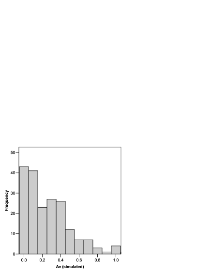
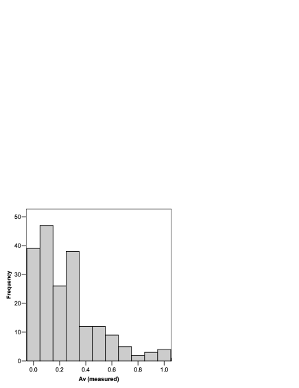
The distribution of the internal extinction can be easily modelled by random orientation of a dusty galactic disc to the line of sight222This is of course a very crude approximation since the morphological types of the SN Ia host galaxies show a wide variety of morphologies, including undisturbed ellipticals, spirals and disturbed systems (Farrah et al. [2002]).. Assuming that the SN Ia supernovae belong to the old disc population with a scale height of 300 pc (della Valle & Panagia [1992]; Wainscoat et al. [1992] gave 325 pc for the old disc population) and the dust layer in the disc have a scale height of about 130 pc and 0.18 mag visual extinction perpendicular to the symmetry plane one gets the simulated distribution as displayed in the upper panel of Figure 1. The lower panel of Figure 1 shows the distribution of observed extinctions for comparison. The pronounced peak at the low extinction part of the histogram is probable accounted for supernovae in front side of the host galaxy while the second less pronounced one is caused by those at the opposite side. The observed distribution is probable biased at the high redshift part of the sample towards lower extinctions because close to the limit of detection the heavily obscured supernovae can be missed by the observation. Despite of the simplicity of the model applied the simulated data reproduce remarkably well the basic characteristics of the observed distribution within the limits of statistical inference. A Kolmogorov-Smirnov test revealed that the difference between the simulated and measured distributions can be accounted for chance with a probability.
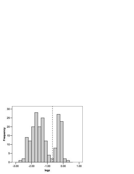
The redshift distribution of the sample is bimodal (see Fig. 2). There is a dip at z = 0.25 splitting the data set into a low and a high redshift part. In the low redshift domain the luminosity distances derived from various cosmological models differ only within the statistical uncertainty of estimating them directly from SN Ia events. At the same time, the accuracy of the measurements allows us to distinguish between cosmological models in the range. Assuming that is given, the SN Ia luminosity distance, derived from an empty Universe, represents an upper bound among those obtained from cosmological models. In what follows, we consider this bound as a reference distance at a given . If the distances obtained from SN Ia observation exceeded significantly this bound the introduction of a nonzero cosmological constant seems to be inevitable.
Tonry et al. ([2003]) multiplied the luminosity distances by the present value of the Hubble constant and listed their logarithm, along with the estimated uncertainty.
For further statistical studies we calculated the standardized deviation from an empty model, where is the measured logarithmic luminosity distance as given in Tonry et al. ([2003]), the corresponding measurement error and the calculated logarithmic distance in a given model universe.
where and is defined as , and for and , respectively.
The deviations of the measured distances from the calculated ones, based on some cosmological model, distributed symmetrically in the case of a good fit. In the following we performed several sign tests for the whole sample and several subsamples splitting the original one with and the median of the extinction. We use the median instead of the sample mean value because the former is less sensitive to outliers. Table 1 shows these quantities for the two redshift range defined and the whole sample, respectively.
| redshift | Mean | Median | N |
|---|---|---|---|
| 0.306 | 0.250 | 140 | |
| 0.194 | 0.140 | 61 | |
| Total | 0.272 | 0.190 | 201 |
2.2 Performing tests on the data
A combination of the median of internal extinction and the cut, divided the data set into four subsamples. We used sign tests to study whether the distribution of the standardized residuals, introduced in the 2.1 subsection, was symmetric in relation to the level defined by the empty model, within these subsamples. A significant excess of the ”+” signs favors a model and in the opposite case one gets support for traditional Friedmann solutions.
We made the assumption that the probability of the ”+” (or ”-”) signs of the residuals followed a Binomial distribution in the form of:
| (2) |
where means the number of trials, that of successes and is the probability of one of these events ( in symmetric case). The mean value of successes is given by . One may compute the probability of the deviation from the mean assuming that it happens only by chance:
| (3) |
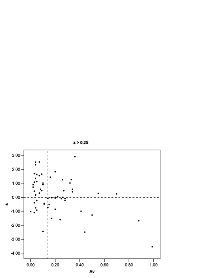
The formula given by Equation (3) has the advantage that it is exact and works correctly even in the case of a small sample size. We carried out sign tests on the subsamples defined by cutting the data set at the median in the low and high redshift part, separately. Tables 2 and 3 summarize the results. As Table 2 demonstrates the subsamples are symmetric, independently of the internal extinction. On the contrary, the results summarized in Table 3 indicates a difference in the statistical properties of the low and high extinction part of the subsample (see Figure 3). While the low extinction part clearly shows an excess of the points above the reference line it is not the case among the points above the median. This fact indicates some sort of interrelation between the internal extinction and the standardized residuals in the high domain.
| k (”-”) | n-k (”+”) | n | ||
|---|---|---|---|---|
| 34 | 35 | 69 | 1.000 | |
| 34 | 37 | 71 | 0.813 | |
| Total | 68 | 72 | 140 | 0.800 |
| k (”-”) | n-k (”+”) | n | ||
|---|---|---|---|---|
| 9 | 21 | 30 | 0.043 | |
| 17 | 14 | 31 | 0.720 | |
| Total | 26 | 35 | 61 | 0.305 |

The sign test is appropriate for studying the significance of the excess of points above the line and could give a clear support for cosmology. One may wonder, however, whether additional statistical tests also confirm the result obtained from the sign test. To proceed in this way we performed three additional tests on the high part of the sample: Student’s , Mann-Whittney and Kolmogorov-Smirnov tests. The Student’s test compares the means while the others the distribution of at both side of the median of . We summarized the results in Table 4.
| Type of test | sign. | No. of objects |
|---|---|---|
| Student’s | 0.044 | 61 |
| Mann-Whittney | 0.025 | 61 |
| Kolmogorov-Smirnov | 0.005 | 61 |
One may infer from Table 4 that the results of the additional tests confirm the conclusion obtained from the sign test.
2.3 Pearson’s correlation and factor analysis
To quantify the interrelation pointed out in subsection 2.2 we computed Pearson’s linear correlation between and in the low and high domain, separately. Inspecting Table 5 infers that there is a very significant correlation in the high redshift part unlike the low redshift one.
We made the assumption there was an hidden variable which was present in both and and it was responsible for the interrelation. From strictly statistical point of view, it was not necessary to specify the physical nature of this variable. Following this assumption, the observed and could be expressed in terms of by the following system of equations:
| (4) |
where , are constants and , represent noise terms. To estimate , and we invoked the standard technique of factor analysis. In many statistical software packages (e.g. in the widely used SPSS333SPSS is a registered trade mark for Statistical Package for Social Sciences) the default solution of a factor model is equivalent to the computation of principal components (PC) of the correlation matrix of the observed variables ( and in our case). For obtaining PCs one has to solve the eigenvalue problem of the correlation matrix of the observed variables:
| (5) |
where is the Pearson correlation between and , are the components of the eigenvector, and is the eigenvalue of the matrix.
If one used principal components for establishing a factor model the usual way is to make a distinction between the ’significant’ and ’non-significant’ PCs and keeping only the former ones. A common procedure for making this kind of distinction is to keep only those eigenvectors which belong to eigenvalues above a given threshold. The widely used Kaiser criterion (Kaiser [1960]) keeps eigenvalues of . We used this criterion in our analysis.
The components can be used to obtain the constants in Equation (4) according to the following equalities:
| (6) |
where are the standard deviations of and , respectively. For each data point the value of the variable (the factor score) is resulted with keeping the first PC and ; are the residuals when substituted into Equation (4).
| Sig. (2-tailed) | N | ||
|---|---|---|---|
| -0.068 | 0.427 | 140 | |
| -0.411 | 0.001 | 61 | |
| Total | -0.122 | 0.086 | 201 |
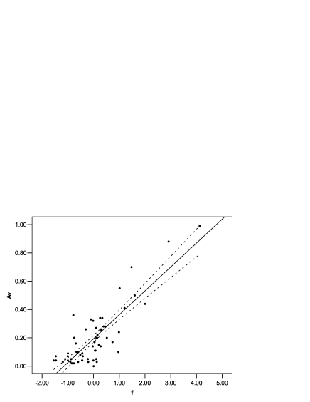
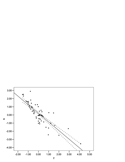
The background variable reproduced well both the internal extinction and the residual as displayed in Figure 4. One has to remove the effect of this variable from the luminosity distances before using them for testing cosmological models.
2.3.1 Caveats
The high level of significance obtained for the Pearson’s correlation has to be treated with some caution. Usually, one assumes that both variables have Gaussian distribution when calculating the significance level of the Pearson’s correlation. In our case this assumption is far from the reality in particular at in the range. There are 57 objects in the part and only 4 with .
If one considered only the data points in the range of the sample the Pearson’s correlation is still negative but drops back to -0.221 with a significance of 0.094.
To get a measure of correlation independent on the assumption of normality we split the sample into four parts with the medians of and . The number of data points in these quadrants form a contingency table. Making use this table one can compute other measures of correlation as listed in Table 6.
| Type of corr. | Sig. | N | |
|---|---|---|---|
| Pearson’s linear ( | -0.411 | 0.001 | 61 |
| Pearson’s linear () | -0.221 | 0.094 | 57 |
| Pearson’s R ( cont. table) | -0.381 | 0.005 | 57 |
| Spearman ( cont. table) | -0.381 | 0.005 | 57 |
One may infer from Table 6 that measure of correlation obtained from the contingency table is close to the Pearson’s linear correlation computed for the whole sample.
3 Testing cosmological models
As we pointed out at the end of Section 2 the luminosity distances had to be freed from the interrelation with the internal extinction, before testing cosmological models. The factor analysis splits the actual residual into two parts: where represents that part explained by the background variable while stands for the true one which is independent from the amount of the internal extinction.
Going back to the definition of as given in Subsection 2.1 we may write . Subtracting from this equation, that part explained by the background variable, we obtain: which is already free from the interrelation with internal extinction. This luminosity distance can be used for testing cosmological models.
The luminosity distance of an object of redshift can be calculated in the framework of a given cosmological model. Besides it depends on and cosmological parameters. It is widely accepted, based on the recent results of SN Ia data and the WMAP project, that and favoring a flat Euclidean model (Hansen et al. [2004]; Verde [2003]; Wright [2003]).
We did not intend to repeat the estimation of and using the original data of Tonry et al. ([2003]) and Barris et al. ([2004]). To make a comparison we used only our corrected data. For this purpose we calculated the distance between our corrected data and those obtained from cosmological models according to the equation below:
| (7) |
Minimizing this distance with respect to gives the best estimate of these parameters according to the observed set of . Assuming that the residuals follow a Gaussian distribution and introducing the likelihood function we obtain:
| (8) |
The confidence of the parameters can be estimated making use of the following theorem :
| (9) |
where mean the likelihood function at the maximum and the true value of the parameters estimated, respectively (for the details see Kendall & Stuart [1973]). The degree of freedom is in our case.
Based on our corrected luminosity distances we calculated the best fitting values of by minimizing in Equation (7) and, consequently, maximizing in Equation (8) at the same time.
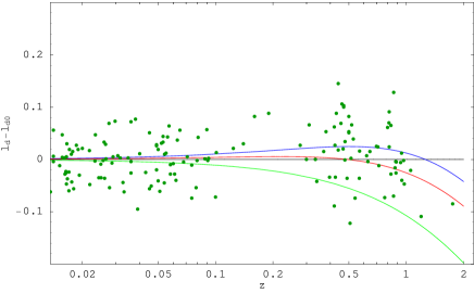
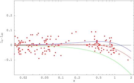
As a best fit we obtained and which considerably differ from the canonical and . In Figure 5 we displayed the scatterplot between and the deviation of the observed luminosity distances and the calculated ones in an empty Universe before (left panel) and after correction (right panel). It is worth noticing the much smaller scatter of the corrected data around the best fitting line in the region in comparison with the non-corrected data. Computing the value for one degree of freedom we obtained for the non-corrected sample and for the corrected one.
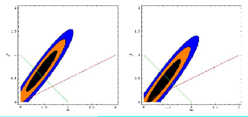
Equation (9) enabled us to calculate the confidence interval of the parameters estimated. After fixing a value for Equation (9) specifies a boundary in the parameter space. The particular value specified for gives a probability that the true value of the estimated parameters are outside and that inside this boundary. gives the confidence level of this region. Following this procedure we calculated the confidence and the result is shown in the right panel of Figure 6. In the left panel of this figure we also give the confidence of the parameters using the uncorrected sample for comparison.
A comparison of the left and the right panel of Figure 6 clearly shows the basic difference between the parameters obtained from the uncorrected and corrected data. While the uncorrected data strongly supports the solution is well within the 95% confidence region in the corrected case. It is also important to note that the canonical and solution is outside of the 99% confidence region of the corrected data. However, the line referring to an Euclidean Universe crosses the confidence region with a best estimate of and values.
The statistical results obtained in Section 2 are purely phenomenological and give no hint of the probable reason of the interrelation between the luminosity distance and internal extinction as given in the data set of Tonry et al. ([2003]) and Barris et al. ([2004]). A detailed careful simulation of the procedure of obtaining the luminosity distance and internal extinction would be desirable to uncover the probable reason of the interrelation found in Section 2. A detailed study of this kind may reveal whether this interrelation has some astrophysical reason or is purely a byproduct of the procedure for obtaining the luminosity distance and internal extinction.
4 Summary and Conclusions
We studied the basic statistical properties of the SN Ia sample published by Tonry et al. ([2003]) and Barris et al. ([2004]). The observed distribution of the internal extinction due to the host galaxies can be well modelled by a dusty disc oriented randomly to the line of sight. We divided the sample into the low and high part at a dip in the distribution at .
We further divided the low and the high redshift part of the sample by the median of the internal extinction. Four subsamples resulted in this way. We selected the redshift - luminosity distance relationship of an empty Universe as a reference level and calculated the standardized deviation of the logarithmic luminosity distances of Tonry et al. ([2003]) and Barris et al. ([2004]) from those of the empty model.
Performing sign tests on the standardized residuals, on the four subsamples separately, revealed that is distributed symmetrically in the low redshift () part of the sample, independently on the internal extinction. On the other hand, the low extinction part of the data of clearly showed an excess of the points of which was not the case among those of having extinction above the median. This diversity in the behavior of the points below and above the median pointed to an interrelation between the residual and the internal extinction.
To characterize quantitatively the interrelation between and we computed the Pearson’s linear correlation in the low and the high redshift part, separately. Assuming that the interrelation can be represented by a hidden common variable in and we constructed a factor model for explaining the observed variables. We used PCA and the Kaiser criterion for verifying the factor model.
After subtracting that part of the residual which was explained by the factor model we obtained a corrected sample, free already from the interrelation between and . Minimizing the distance between the corrected data and a cosmological model with respect to one may conclude that there was no need for .
We have to emphasize, however, than one came to this conclusion assigning the same weight to the low and higher extinction part of the sample in the region. Nevertheless, some concerns can be made for the reliability of the estimated extinction in the host galaxy. Without the proposed correction the low extinction part of the sample clearly supports the cosmology.
Our result was purely phenomenological based only on the statistical properties of the data. Consequently, further detailed studies are required whether the interrelation between the luminosity distance and the internal extinction in the high part of the sample has an astrophysical meaning or is simply a byproduct of the way as and were obtained from the data.
Acknowledgements.
This work was supported by the OTKA grant T048870. We are grateful to P.G. Teres for carefully reading the manuscript and suggesting valuable improvements. Zs. Hetesi is indebted to B. Balázs for numerous discussions.References
- [2006] Astier, P., Guy, J., Regnault, N., et al.: 2006, A&A 447, 31
- [2004] Barris, B. J., Tonry, J. L., Blondin, S., et al.: 2004, ApJ 602, 571
- [1992] Carroll, S. M., Press, W. H., Turner, E. L.: 1992, ARA&A 30, 499
- [2004] Clements, D. L., Farrah, D., Fox, M., Rowan-Robinson, M., Afonso, J.: 2004, NewAR 48, 629
- [1992] della Valle, M. & Panagia, N.: 1992, AJ 104, 696
- [2002] Farrah, D. M., Meikle, W. P. S., Clements, D., Rowan-Robinson, M., Mattila, S.: 2002, MNRAS 336, L17
- [2004] Farrah, D., Fox, M., Rowan-Robinson, M., Clements, D., Afonso, J.: 2004, ApJ 603, 489
- [2001] Gott, J.R., Vogeley, M.S., Podariu, S., Ratra, B.: 2001, ApJ 549, 1
- [2004] Hansen, F. K., Balbi, A., Banday, A. J., Górski, K. M.: 2004, MNRAS354, 905
- [2005] Hetesi, Zs. & Bal zs, L.G.: 2005, Publications of the Astronomy Department of the E tv s University (PADEU), Vol. 15., p. 159
- [2005] Jain, P. & Ralston, J.P.: 2005, astro-ph/0506478
- [1960] Kaiser, H.F.: 1960, Educational and Psychological Measurement 20, 141
- [1973] Kendall, M.G., & Stuart, A.: 1973, ’The Advanced Theory of Statistics’, Charles Griffin & Co. Ltd., London &High Wycombe
- [2003] Knop, R.A., Aldering, G., Amanullah, R., et al.: 2003, ApJ 598, 102
- [2001] Leibundgut, B.: 2001, ARA&A 39, 67
- [2002] Mészáros, A.: 2002, ApJ 580, 12
- [1999] Perlmutter, S., Aldering, G., Goldhaber, G., et al.: 1999, ApJ 517, 565
- [2005] Reindl, B., Tammann, G. A., Sandage, A., Saha, A.: 2005, ApJ 624, 532
- [1996] Riess, A.G., Press, W.H., Kirshner, R.P.: 1996, ApJ 473, 588
- [1998] Riess, A.G., Filippenko, A.V., Challis, P., et al.: 1998, AJ 116, 1009
- [2004] Riess, A.G., Strolger, L.-G., Tonry, J., et al.: 2004, ApJ 607, 665
- [2002] Rowan-Robinson, M.: 2002, MNRAS 332, 352
- [2003] Tonry, J.L., Schmidt, B.P., Barris, B., et al.: 2003, ApJ 594, 1
- [1998] Schlegel, D.J., Finkbeiner, D. P., Davis, M.: 1998, ApJ 500, 525
- [2003] Verde, L.: 2003, NewAR, 47, 713
- [1992] Wainscoat, R.J., Cohen, M., Volk, K., et al.: 1992, ApJS 83, 111
- [2003] Wright, E. L.: 2003, NewAR 47, 877