Two 3-Branes in Randall-Sundrum Setup and Current Acceleration of the Universe

Abstract

Five-dimensional spacetimes of two orbifold 3-branes are studied, by assuming that the two 3-branes are spatially homogeneous, isotropic, and independent of time, following the so-called “bulk-based” approach. The most general form of the metric is obtained, and the corresponding field equations are divided into three groups, one is valid on each of the two 3-branes, and the third is valid in the bulk. The Einstein tensor on the 3-branes is expressed in terms of the discontinuities of the first-order derivatives of the metric coefficients. Thus, once the metric is known in the bulk, the distribution of the Einstein tensor on the two 3-branes is uniquely determined. As applications, we consider two different cases, one is in which the bulk is locally $AdS_{5}$, and the other is where it is vacuum. In some cases, it is shown that the universe is first decelerating and then accelerating. The global structure of the bulk as well as the 3-branes is also studied, and found that in some cases the solutions may represent the collision of two orbifold 3-branes. The applications of the formulas to the studies of the cyclic universe and the cosmological constant problem are also pointed out.

I Introduction

Superstring and M-theory all suggest that we may live in a world that has more than three spatial dimensions.  Because only three of these are presently observable, one has to explain why the others are hidden from detection.  One such explanation is the so-called Kaluza-Klein (KK) compactification, according to which the size of the extra dimensions is very small (often taken to be on the order of the Planck length).  As a consequence, modes that have momentum in the directions of the extra dimensions are excited at currently inaccessible energies.

Recently, the braneworld scenarios ADD ; RS1 has dramatically changed this point of view and, in the process, received a great deal of attention. At present, there are a number of proposed models  (See, for example, reviews and references therein.). In particular, Arkani-Hamed et al (ADD) ADD pointed out that the extra dimensions need not necessarily be small and may even be in the scale of millimeters Hoyle04 .  This model assumes that Standard Model fields are confined to a three (spatial) dimensional surface (a 3-brane) living in a larger dimensional bulk, while the gravitational field propagates in the whole bulk.  Additional fields may live only on the brane or in the whole bulk, provided that their current undetectability is consistent with experimental bounds. One of the most attractive features of this model is that it may potentially resolve the long standing hierarchy problem, namely the large difference in magnitudes between the Planck and electroweak scales.

An alternative approach was proposed by Randall and Sundrum (RS) RS1 , which will be referred to as RS1 model. One of the most attractive features of this model is that it will soon be explored by LHC DHR00 . For critical reviews of the model and some open issues, we refer readers to RC04 . The spacetime in this model is five-dimensional, with the extra dimension being compactified on an $S^{1}/Z_{2}$ orbifold, that is, the extra dimension is periodic, $\phi\in[-\pi,\pi]$, and its points with ($x^{\mu},\phi$) are identified with the ones ($x^{\mu},-\phi$). In such a setting, the spacetime necessarily contains two 3-branes, located, respectively, at the fixed points $\phi=0$, and $\phi=\pi$. The brane at $\phi=0$ is usually called hidden (or Planck) brane, and the one at $\phi=\pi$ is called visible (or TeV) brane. The corresponding 5D spacetime is locally anti-de Sitter ($AdS_{5}$), and described by the metric,

$$ds^{2}_{5}=e^{-2kr_{c}|\phi|}\eta_{\mu\nu}dx^{\mu}dx^{\nu}-r^{2}_{c}d\phi^{2},$$ (1.1)

for which the 4D spacetimes of the two 3-branes are Poincaré invariant, where $\mu,\;\nu=0,1,2,3$, and $k$ is a constant and of the order of $M$, where $M$ is the five-dimensional mass scale. $\eta_{\mu\nu}$ denotes the 4D Minkowski metric, and $r_{c}$ the radius of the extra dimension. To obtain the relationship between $M$ and the four-dimensional Planck scale $M_{pl}$, let us consider the gravitational perturbations, given by

$$ds^{2}_{5}=e^{-2kr_{c}|\phi|}\left[\eta_{\mu\nu}+h_{\mu\nu}\left(x^{\lambda}\right)\right]dx^{\mu}dx^{\nu}-r^{2}_{c}d\phi^{2},$$ (1.2)

we find that

$$S^{(5)}_{g} = \frac{M^{3}}{16\pi}\int{dx^{4}d\phi\sqrt{g^{(5)}}R^{(5)}}$$

$$= \frac{M^{3}}{16\pi}\int{d^{4}x}\int^{\pi}_{-\pi}{d\phi r_{c}e^{-2kr_{c}|\phi|}\sqrt{-g^{(4)}}R^{(4)}},$$

where $g^{(4)}\equiv\eta_{\mu\nu}+h_{\mu\nu}$. Then, comparing Eq.(I) with

$$S_{g}^{(4)}=\frac{M^{2}_{pl}}{16\pi}\int{d^{4}x\sqrt{-g^{(4)}}R^{(4)}},$$ (1.4)

we find that

$$M^{2}_{pl}=\frac{M^{3}}{k}\left(1-e^{-2kr_{c}\pi}\right).$$ (1.5)

Thus, in the RS1 model, for large $kr_{c}$ the Planck $M_{pl}$ is weakly dependent on $r_{c}$ and $M_{pl}\sim M$. Therefore, in contrast to the ADD model, the RS1 model predicts that $M$ and $M_{pl}$ are in the same order, $M\sim M_{pl}\sim 10^{16}\;TeV$. The resolution of the hierarchy problem comes from the warped factor $e^{-2kr_{c}\pi}$ on the visible brane. To show this explicitly, let us consider a scalar field $H$ confined on the brane,

$$S_{eff.}^{vis} = \int_{\phi=\pi}{d^{4}x\sqrt{-g_{vis}}\left[g^{\mu\nu}_{vis}\nabla_{\mu}H^{*}\nabla_{\nu}H\right.}$$ (1.6)

$${\left.-\lambda\left(\left|H\right|^{2}-m^{2}_{0}\right)^{2}\right]}$$

$$= \int_{\phi=\pi}{d^{4}x\left[g^{\mu\nu}\nabla_{\mu}{\bar{H}}^{*}\nabla_{\nu}{\bar{H}}\right.}$$

$$\left.-\lambda\left(\left|{\bar{H}}\right|^{2}-e^{-2k\pi r_{c}}m^{2}_{0}\right)^{2}\right],$$

where ${\bar{H}}\equiv e^{k\pi r_{c}}H$, and

$$g_{vis}^{\mu\nu}\equiv g_{5}^{\mu\nu}(x,\pi)=e^{2k\pi r_{c}}g^{\mu\nu}.$$ (1.7)

Therefore, the mass measured by $g_{\mu\nu}$ is given by

$$m=e^{-k\pi r_{c}}m_{0}.$$ (1.8)

Then, for $kr_{c}\sim 11$ and $m_{0}\sim 10^{16}\;TeV$, we find $m\sim TeV$.

When extra dimensions exist, a critical ingredient is the stability of the extra dimensions. Goldberger and Wise showed that values of $kr_{c}\sim 11$ are indeed natural and can be provided by a stable configuration GW99 .

In this paper, we study cosmological models in the RS1 setup. In the original model, only gravity propagated in the bulk and the standard model fields were confined to the TeV brane. As a results, the bulk is necessarily a generalized Schwarzschild-anti-de Sitter space KI99 . However, soon it was realized that much richer phenomena can be obtained, if some of the standard model fields are allowed to propagate in the bulk DHR00 . In order to incorporate all these situations, we shall allow the bulk to be filled with any matter field(s).

In addition, much of the work in brane cosmology has taken the so-called “brane-based” approach reviews ; RS1CMs . In this paper, we shall follow the “bulk-based” approach BCG00 , initiated by the authors of KI99 . In BCG00 spacetimes with one 3-brane were studied systematically by the “bulk-based” approach, and in particular the most general form of the bulk metric was found. In this paper, we shall generalize those studies to the case of two 3-branes. As shown explicitly in Sec. II, their general form of the bulk metric is a particular case of ours for two 3-branes.

The rest of the paper is organized as follows: In Sec. II, starting with the assumption that the two orbifold 3-branes are spatially homogeneous, isotropic, and independent of time, and that the extra dimension has $S^{1}/Z_{2}$ symmetry, we derive the most general form of the metric. It is very important to note that the orbifold symmetry manifests itself explicitly only in certain coordinate system. In this paper, we take the point of view that this particular coordinate system is the one in which the two 3-branes are all at rest. With this in mind, using gauge freedom we first map the two 3-branes into fixed points, in which the proper distance between the two 3-branes in general is time-dependent. Then, using distribution theory we develop a general formula for two 3-branes with orbifold symmetry. In particular, we divide the field equations into three different groups, given, respectively, by Eqs.(2.25), (2.26) and (2.27), where Eq.(2.25) holds in the bulk, and Eqs.(2.26) and (2.27) hold on each of the two 3-branes. The Einstein tensor on the two 3-branes is given in terms of the discontinuities of the metric coefficients. Thus, once the metric is known in the bulk, $G^{(0)}_{AB}$ and $G^{(c)}_{AB}$ are known, and Eqs.(2.26) and (2.27) will uniquely determine the distribution of the matter fields on the two 3-branes. In Sec. III, as applications of our general formulas, we consider two 3-branes in an $AdS_{5}$ bulk, by imposing the conditions that the cosmological constant on the visible brane vanishes and the equation of state of its matter field is given by $p_{c}=w\rho_{c}$, with $w$ being a constant. From this example we can see that different “cut-paste” operations result in different models, even although the bulks are all locally anti-de Sitter. The global structure of the bulk and the 3-branes is also studied, and found that in some cases the geodesically complete spacetime represents infinite number of 3-branes. In Sec. IV, similar considerations are carried out, but now the bulk is vacuum. After re-deriving the general vacuum solutions of the five-dimensional bulk BCG00 , we apply our general formulas to these solutions for two 3-branes, and whereby obtain the conditions under which the universe undergoes a current acceleration. The study of global structure of these solutions shows that some solutions may represent the collision of two orbifold 3-branes. Sec. V contains our main conclusions and remarks.

It should be noted that the problem has been studied so intensively, there is inevitably overlap between previous works and what we present here. However, as far as we know, it is the first time to present such a general treatment of two orbifold 3branes in arbitrary bulks and systematically study the global structures of the bulk for all the solutions with/without the bulk cosmological constant.

II Gauge Freedom and Gauge Choice For Two Homogeneous and Isotropic 3-Branes

In this paper we consider spacetimes that are five-dimensional and contain two 3-branes. Since we shall apply such spacetimes to cosmology, we further assume that the two 3-branes are spatially homogeneous, isotropic, and independent of time. The fifth dimension is periodic and has a reflection (orbifold) symmetry with respect to each of the two 3-branes. Then, one can see that the space between the two 3-branes represents half of the periodic space along the fifth dimension.

To start with, let us first consider the conditions that the space on the two 3-branes is spatially homogeneous, isotropic, and independent of time. It is not difficult to show that such a space must have a constant curvature at any point of the two 3-branes, and its metric must take the form Wolf ,

$$d\Sigma^{2}_{k}\equiv\gamma_{ab}dx^{a}dx^{b}=\frac{dr^{2}}{1-kr^{2}}+r^{2}d\Omega^{2},$$ (2.1)

where $d\Omega^{2}\equiv d\theta^{2}+\sin^{2}\theta d\phi^{2}$, and $a,b=1,2,3$. The constant $k$ represents the curvature of the 3-space, and can be positive, negative or zero. Without loss of generality, we shall choose coordinates such that $k=0,\pm 1$. Then, one can see that the most general metric for the five-dimensional spacetime must take the form,

$$ds^{2}_{5}=g_{AB}dx^{A}dx^{B}=g_{ij}dx^{i}dx^{j}-A^{2}(x^{i})d\Sigma^{2}_{k},$$ (2.2)

where $i,j=0,4,\;A,B=0,1,2,3,4$, and $d\Sigma^{2}_{k}$ is given by Eq.(2.1). In such coordinates, the two 3-branes are located on the hypersurfaces

$$\phi_{1}\left(x^{i}\right)=0,\;\;\;\phi_{2}\left(x^{i}\right)=0,$$ (2.3)

as shown by Fig. 1(a). Clearly, the metric (2.2) is invariant under the coordinate transformation,

$${x^{\prime}}^{i}=f^{i}\left({x}^{j}\right).$$ (2.4)

As mentioned in the last section, the orbifold symmetry manifests itself explicitly only in coordinates in which the two 3-branes are all at rest. Therefore, before imposing such a symmetry, using one degree of the freedom of Eq.(2.4), we first map the two 3-branes to the fixed points $y=0$ and $y=y_{c}$, for example, by setting

$$y=\frac{\phi^{\alpha}_{1}}{\phi^{\alpha}_{1}+\beta\phi^{\gamma}_{2}}y_{c},$$ (2.5)

where $y_{c},\;\alpha,\;\beta$ and $\gamma$ are arbitrary constants [cf. Fig. 1(b)]. Without loss of generality, in this paper we assume $y_{c}>0$ and consider the brane located in this surface as our TeV brane. Clearly, by properly choosing these constants, the above coordinate transformation is non-singular NoteA . Then, we can use the other degree of freedom of Eq.(2.4) to set $g_{04}=0$, so that the metric can be cast in the form,

$$ds^{2}_{5}=N^{2}\left(t,y\right)dt^{2}-A^{2}\left(t,y\right)d\Sigma^{2}_{k}-B^{2}\left(t,y\right)dy^{2}.$$ (2.6)

It should be noted that in BCG00 the authors used the two degrees of freedom of Eq.(2.4) to set $N(t,y)=B(t,y)$ and $g_{ty}=0$ for the case of one 3-brane. In such chosen ($t,y$)-coordinates, the 3-brane in general is located on the hypersurface $y=\chi(t)$. Then, using the remaining gauge freedom, $t=t^{\prime}+[\chi(t^{\prime}+y^{\prime})-\chi(t^{\prime}-y^{\prime})]/2$, and $y=y^{\prime}+[\chi(t^{\prime}+y^{\prime})+\chi(t^{\prime}-y^{\prime})]/2$, one can bring the 3-brane to the fixed point $y^{\prime}=0$, while still keep the metric in the same form in terms of $t^{\prime}$ and $y^{\prime}$. For details, we refer readers to BCG00 . Clearly, this is possible only for the case of one 3-brane. For the case of two 3-branes, in general we have $N(t,y)\not=B(t,y)$, as shown above.

Figure 1: The trajectories of two orbifold 3-branes: (a) In the ($x^{0},x^{4}$)-plane. (b) In the ($t,y$)-plane, in which the two 3-branes are at rest, but the proper distance between then in general is time-dependent.

The non-vanishing components of the Einstein tensor for the metric (2.6) are given by

$$G_{00} = -3\frac{N^{2}}{B^{2}}\left\{\frac{A_{,yy}}{A}+\frac{A_{,y}}{A}\left(\frac{A_{,y}}{A}-\frac{B_{,y}}{B}\right)\right\}$$

$$+3\frac{A_{,t}}{A}\left(\frac{A_{,t}}{A}+\frac{B_{,t}}{B}\right)+3k\frac{N^{2}}{A^{2}},$$

$$G_{04} = -3\left\{\frac{A_{,ty}}{A}-\frac{A_{,t}}{A}\frac{N_{,y}}{N}-\frac{B_{,t}}{B}\frac{A_{,y}}{A}\right\},$$

$$G_{ab} = \frac{A^{2}}{B^{2}}\gamma_{ab}\left\{2\frac{A_{,yy}}{A}+\frac{N_{,yy}}{N}+\frac{A_{,y}}{A}\left(\frac{A_{,y}}{A}-2\frac{B_{,y}}{B}\right)\right.$$

$$\left.+\frac{N_{,y}}{N}\left(2\frac{A_{,y}}{A}-\frac{B_{,y}}{B}\right)\right\}$$

$$-\frac{A^{2}}{N^{2}}\gamma_{ab}\left\{2\frac{A_{,tt}}{A}+\frac{B_{,tt}}{B}+\frac{A_{,t}}{A}\left(\frac{A_{,t}}{A}+2\frac{B_{,t}}{B}\right)\right.$$

$$\left.-\frac{N_{,t}}{N}\left(2\frac{A_{,t}}{A}+\frac{B_{,t}}{B}\right)\right\}-k\gamma_{ab},$$

$$G_{44} = -3\frac{B^{2}}{N^{2}}\left\{\frac{A_{,tt}}{A}+\frac{A_{,t}}{A}\left(\frac{A_{,t}}{A}-\frac{N_{,t}}{N}\right)\right\}$$ (2.7)

$$+3\frac{A_{,y}}{A}\left(\frac{A_{,y}}{A}+\frac{N_{,y}}{N}\right)-3k\frac{B^{2}}{A^{2}},$$

where $F_{,y}\equiv\partial F/\partial y$, etc.

The reflection symmetry with respect to the two branes can be obtained by the replacement

$$y\rightarrow\left|y\right|,$$ (2.8)

so that the most general metric for two 3-branes finally takes the form,

$$ds^{2}_{5}=N^{2}\left(t,\left|y\right|\right)dt^{2}-A^{2}\left(t,\left|y\right|\right)d\Sigma^{2}_{k}-B^{2}\left(t,\left|y\right|\right)dy^{2},$$ (2.9)

where

$$\left|y\right| \equiv \cases{...&, ...,\cr y+2y_{c}&, $-2y_{c}\leq y\leq-y_{c}$,\cr-y&, $-y_{c}\leq y\leq 0$,\cr y&, $0\leq y\leq y_{c}$,\cr 2y_{c}-y&, $y_{c}\leq y\leq 2y_{c}$,\cr...&, ...,\cr}$$ (2.10)

$$= \sum^{\infty}_{n=-\infty}{\left(2ny_{c}-y\right)H\left(y-\left(2n-1\right)y_{c}\right)}$$

$$\;\;\;\;\;\;\;\;\;\;\;\times\left[1-H\left(y-2ny_{c}\right)\right]$$

$$+\sum^{\infty}_{n=-\infty}{\left(y-2ny_{c}\right)H\left(y-2ny_{c}\right)}$$

$$\;\;\;\;\;\;\;\;\;\;\;\;\times\left[1-H\left(y-\left(2n+1\right)y_{c}\right)\right],$$

as shown in Fig. 2, where $H(x)$ denotes the Heavside function, defined by,

$$H(x)=\cases{1,&$x>0$,\cr 0,&$x<0$.\cr}$$ (2.11)

Hence, we obtain

$$\frac{d|y|}{dy} = \sum^{\infty}_{n=-\infty}{-H\left(y-\left(2n-1\right)y_{c}\right)}$$

$$\;\;\;\;\;\;\;\;\;\;\;\times\left[1-H\left(y-2ny_{c}\right)\right]$$

$$+\sum^{\infty}_{n=-\infty}{H\left(y-2ny_{c}\right)}$$

$$\;\;\;\;\;\;\;\;\;\;\;\;\times\left[1-H\left(y-\left(2n+1\right)y_{c}\right)\right],$$

$$\frac{d^{2}|y|}{dy^{2}} = 2\sum^{\infty}_{n=-\infty}{\delta(y-2ny_{c})}$$ (2.12)

$$-2\sum^{\infty}_{n=-\infty}{\delta\left(y-(2n+1)y_{c}\right)},$$

where $\delta(x)$ denotes the Dirac function, with

$$\frac{dH(x)}{dx} = \delta(x),$$

$$\int^{\infty}_{-\infty}{f(x)\delta(x)dx} = f(0),$$ (2.13)

for any given test function $f(x)$.

Figure 2: The function $\left|y\right|$ defined by Eq.(2.10).

However, the orbifold symmetry first restricts $y$ to the range, $-y_{c}\leq y\leq y_{c}$, and then identifies the points $\left(x^{\mu},\;y\right)$ with the ones $\left(x^{\mu},\;-y\right)$, so that $y$ finally takes its values only in the range, $0\leq y\leq y_{c}$. Then, Eq.(II) yields

$$\frac{d|y|}{dy} = 1,$$

$$\frac{d^{2}|y|}{dy^{2}} = 2\delta(y)-2\delta\left(y-y_{c}\right),$$ (2.14)

for $y\in[0,y_{c}]$.

It should be noted that, although the two 3-branes are all at rest in the above chosen gauge, which will be referred to as the canonical gauge, the proper distance between them in general is time-dependent, and given by

$${\cal{D}}(t)=\int^{y_{c}}_{0}{B(t,y)dy}.$$ (2.15)

The moment where ${\cal{D}}(t)=0$ is the one when the two 3-branes collide.

We also note that the expressions given by Eq.(II) for the Einstein tensor hold even for spacetimes with orbifold symmetry, but now in the sense of distribution. To see this, let us consider a given function $F(t,|y|)$, for which we find

$$\frac{\partial F(t,|y|)}{\partial t} = \frac{\partial F(t,y)}{\partial t},$$

$$\frac{\partial F(t,|y|)}{\partial y} = \frac{\partial F(t,y)}{\partial y},$$

$$\frac{\partial^{2}F(t,|y|)}{\partial t\partial y} = \frac{\partial^{2}F(t,y)}{\partial t\partial y},$$

$$\frac{\partial^{2}F(t,|y|)}{\partial t^{2}} = \frac{\partial^{2}F(t,y)}{\partial t^{2}},$$

$$\frac{\partial^{2}F(t,|y|)}{\partial y^{2}} = \frac{\partial^{2}F(t,y)}{\partial y^{2}}+\left[F_{,y}\right]_{0}\delta(y)$$ (2.16)

$$+\left[F_{,y}\right]_{c}\delta\left(y-y_{c}\right),$$

for $y\in\left[0,y_{c}\right]$, where

$$\left[F_{,y}\right]_{0} \equiv \lim_{y\rightarrow 0^{+}}{\frac{\partial F(t,y)}{\partial y}}-\lim_{y\rightarrow 0^{-}}{\frac{\partial F(t,-y)}{\partial y}}$$

$$= 2\left.\frac{\partial F(t,y)}{\partial y}\right|_{y=0^{+}},$$

$$\left[F_{,y}\right]_{{c}} \equiv \lim_{y\rightarrow y_{c}^{+}}{\frac{\partial F(t,2y_{c}-y)}{\partial y}}-\lim_{y\rightarrow y_{c}^{-}}{\frac{\partial F(t,y)}{\partial y}}$$ (2.17)

$$= -2\left.\frac{\partial F(t,y)}{\partial y}\right|_{y=y_{c}^{-}}.$$

Note that in writing Eq.(II) we had assumed that the derivatives of $F(t,|y|)$ exist from each side of the limits. It can also be shown that

$$H^{m}(x)=H(x),\;\;\;\left[1-H(x)\right]^{m}=1-H(x),$$

$$H(x)\left[1-H(x)\right]=0,\;H(x)\delta(x)=\frac{1}{2}\delta(x),$$

$$\left[F^{+}(x)H(x)+F^{-}(x)\left(1-H(x)\right)\right]\delta(x)$$

$$\;\;\;\;\;\;\;\;\;=\frac{1}{2}\left[F^{+}(0)+F^{-}(0)\right]\delta(x),$$ (2.18)

in the sense of distributions, where $m$ is an integer, and

$$F^{+}(0) \equiv \lim_{x\rightarrow 0^{+}}{F^{+}(x)},$$

$$F^{-}(0) \equiv \lim_{x\rightarrow 0^{-}}{F^{-}(x)}.$$ (2.19)

Inserting Eqs.(II) - (II) into Eq.(II), we find that the Einstein tensor corresponding to the metric (2.9) can be written as

$$G_{AB}=G_{AB}^{(D)}+G_{AB}^{(0)}\delta(y)+G_{AB}^{(c)}\delta\left(y-y_{c}\right),$$ (2.20)

for $y\in[0,y_{c}]$, where $G_{AB}^{(D)}$ denotes the Einstein tensor calculated in the region $y\in\left(0,y_{c}\right)$ and given by Eq.(II), and

$$G_{AB}^{(0)} = \frac{A^{2}_{0}}{B^{2}_{0}}\left(2\frac{\left[A_{,y}\right]_{0}}{A_{0}}+\frac{\left[N_{,y}\right]_{0}}{N_{0}}\right)\gamma_{ab}\delta^{a}_{A}\delta^{b}_{B}$$ (2.21)

$$-3\frac{N^{2}_{0}}{B^{2}_{0}}\frac{\left[A_{,y}\right]_{0}}{A_{0}}\delta^{0}_{A}\delta^{0}_{B},$$

$$G_{AB}^{(c)} = \frac{A^{2}_{c}}{B^{2}_{c}}\left(2\frac{\left[A_{,y}\right]_{c}}{A_{c}}+\frac{\left[N_{,y}\right]_{c}}{N_{c}}\right)\gamma_{ab}\delta^{a}_{A}\delta^{b}_{B}$$ (2.22)

$$-3\frac{N^{2}_{c}}{B^{2}_{c}}\frac{\left[A_{,y}\right]_{c}}{A_{c}}\delta^{0}_{A}\delta^{0}_{B},$$

with

$$F_{0}(t)\equiv F\left(t,0\right),\;\;\;F_{c}(t)\equiv F\left(t,y_{c}\right),$$ (2.23)

where $F\equiv\left\{N,A,B\right\}$. Assuming that the energy-momentum tensor (EMT) takes the form,

$$T_{AB} = T_{AB}^{(D)}+\frac{1}{B_{0}(t)}T_{AB}^{(0)}\delta(y)$$ (2.24)

$$+\frac{1}{B_{c}(t)}T_{AB}^{(c)}\delta\left(y-y_{c}\right),$$

where $T_{AB}^{(D)}$ denotes the bulk EMT, and $T_{AB}^{(0)}$ and $T_{AB}^{(c)}$ the EMT’s of the two 3-branes, the Einstein equations take the form,

$$G_{AB}^{(D)} = \kappa_{5}T_{AB}^{(D)}+\Lambda g_{AB},\;\;y\in\left(0,y_{c}\right),$$ (2.25)

$$G_{\mu\nu}^{(0)} = \frac{1}{B_{0}(t)}\left(\kappa_{5}T_{\mu\nu}^{(0)}+\lambda_{0}g_{\mu\nu}^{(0)}\right),\;\;(y=0),$$ (2.26)

$$G_{\mu\nu}^{(c)} = \frac{1}{B_{c}(t)}\left(\kappa_{5}T_{\mu\nu}^{(c)}+\lambda_{c}g_{\mu\nu}^{(c)}\right),\;\;(y=y_{c}),$$ (2.27)

where

$$g_{\mu\nu}^{(0)}(t)\equiv g_{\mu\nu}(t,0),\;\;\;g_{\mu\nu}^{(c)}(t)\equiv g_{\mu\nu}(t,y_{c}).$$ (2.28)

The constants $\Lambda,\;\lambda_{0}$ and $\lambda_{c}$ denote, respectively, the bulk and the brane cosmological constants. Assuming that the EMT’s of the two 3-branes are given by perfect fluids,

$$T^{(0)}_{\mu\nu} = \left(\rho_{0}+p_{0}\right)u^{(0)}_{\mu}u^{(0)}_{\nu}-p_{0}g_{\mu\nu}^{(0)},$$

$$T^{(c)}_{\mu\nu} = \left(\rho_{c}+p_{c}\right)u^{(c)}_{\mu}u^{(c)}_{\nu}-p_{c}g_{\mu\nu}^{(c)},$$ (2.29)

where

$$u^{(0)}_{\mu}=N_{0}\delta^{0}_{\mu},\;\;\;u^{(c)}_{\mu}=N_{c}\delta^{0}_{\mu},$$ (2.30)

we find that Eqs.(2.26) and (2.27) reduce to

$$\frac{1}{B_{0}}\left(2\frac{\left[A_{,y}\right]_{0}}{A_{0}}+\frac{\left[N_{,y}\right]_{0}}{N_{0}}\right)+\lambda_{0} = \kappa_{5}p_{0},$$

$$\frac{3}{B_{0}}\frac{\left[A_{,y}\right]_{0}}{A_{0}}+\lambda_{0} = -\kappa_{5}\rho_{0},$$ (2.31)

and

$$\frac{1}{B_{c}}\left(2\frac{\left[A_{,y}\right]_{c}}{A_{c}}+\frac{\left[N_{,y}\right]_{c}}{N_{c}}\right)+\lambda_{c} = \kappa_{5}p_{c},$$

$$\frac{3}{B_{c}}\frac{\left[A_{,y}\right]_{c}}{A_{c}}+\lambda_{c} = -\kappa_{5}\rho_{c}.$$ (2.32)

This completes our general description of two homogeneous and isotropic 3-branes with orbifold symmetry, in which the bulk can be filled with any kind of matter fields. In the following, we consider some specific solutions.

III Dynamical Two 3-Branes in $AdS_{5}$

In this section, we first consider the global properties of $AdS_{5}$, and then apply the formulas developed in the last section to study two 3-branes in the background of $AdS_{5}$.

III.1 $AdS_{5}$ Space in Horospheric Coordinates

$AdS_{5}$ can be realized as a hyperboloid embedded in a flat six-dimensional space with two timelike coordinates,

$$\eta_{AB}Y^{A}Y^{B}={\ell}^{-2},\;(A,\;B=0,1,...,5),$$ (3.1)

where $\eta_{AB}=diag\{+1,-1,-1,-1,-1,+1\}$, and ${\ell}\equiv\left(-\Lambda/6\right)^{1/2}$, where $\Lambda$ denotes the cosmological constant of the five-dimensional bulk. In fact, introducing the Einstein universe (EU) coordinates, $\{t_{c},\xi,\theta,\phi,\psi\}$, via the relations,

$${\ell}Y^{0} = \cos t_{c}\sec\xi,$$

$${\ell}Y^{1} = \sin\theta\sin\phi\cos\psi\tan\xi,$$

$${\ell}Y^{2} = \sin\theta\sin\phi\sin\psi\tan\xi,$$

$${\ell}Y^{3} = \sin\theta\cos\phi\tan\xi,$$

$${\ell}Y^{4} = \cos\theta\tan\xi,$$

$${\ell}Y^{5} = -\sin t_{c}\sec\xi,$$ (3.2)

we find that

$$ds^{2}_{5} = \left.\eta_{AB}dY^{A}dY^{B}\right|_{hyperboloid}$$ (3.3)

$$= \frac{1}{\left({\ell}\cos\xi\right)^{2}}\left(dt^{2}_{c}-d\xi^{2}-\sin\xi^{2}d\Omega_{3}^{2}\right)$$

$$\equiv \frac{1}{\left({\ell}\cos\xi\right)^{2}}ds^{2}_{5(E)},$$

where $d\Omega_{3}^{2}[\equiv d\theta^{2}+\sin\theta^{2}d\phi^{2}+\sin\theta^{2}\sin\phi^{2}d\psi^{2}]$ is the line element on the three-sphere $S^{3}$. The range of the EU coordinates that covers the whole $AdS_{5}$ space is $-\pi\leq t_{c}\leq\pi$, $0\leq\xi\leq\pi/2$, $0\leq\theta,\;\phi\leq\pi$, and $0\leq\psi\leq 2\pi$. The timelike hypersurface $\xi=\pi/2$ represents the spatial infinite. The spacelike hypersurfaces $t_{c}=\pm\pi$ are identified, which represent closed timelike curves (CTC’s). The topology of $AdS_{5}$ is $S^{1}$ (time) $\times R^{4}$ (space). To avoid CTC’s for $AdS_{5}$, one may simply unwrap the timelike coordinate $t_{c}$ and extend it to the range, $-\infty<t_{c}<\infty$, so the resulting space has the topology $R^{1}$ (time) $\times R^{4}$ (space), which will be referred to as $CAdS_{5}$. Since the spatial infinity is timelike, neither $CAdS_{5}$ nor $AdS_{5}$ has Cauchy surface. In the rest of this paper, for the sake of simplicity, when we talk about $AdS_{5}$, we always means $CAdS_{5}$.

It is interesting to note that $CAdS_{5}$ covers only half of the static Einstein universe given by $ds^{2}_{5(E)}$ in Eq.(3.3) with the same range for $t_{c},\theta,\phi$ and $\psi$, but now $0\leq\xi\leq\pi$ [cf. Fig. 3].

Figure 3: The $AdS_{5}$ space seen on the Einstein cylinder. The coordinates $\theta,\;\phi$ and $\psi$ are suppressed. Thus, each point represents a three-sphere. The lines $ab$ and $cd$ are identified, which represent CTC’s. Unwrapping $t_{c}$ coordinate and then extending it to the range, $t_{c}\in(-\infty,\infty)$, one can avoid CTC’s. The dotted periodic lines represent timelike geodesics, and the $45^{o}$ straight lines the null geodesics. The vertical line $\xi=\pi/2$ represents the spatial infinity, and a timelike geodesic never reaches it.

To study RS1 model, it is found convenient to introduce the horospheric coordinates, $\{t,x^{1},x^{2},x^{3},z\}$, via the relations,

$${\ell}Y^{0}=-t/z,$$

$${\ell}Y^{i}=x^{i}/z,$$

$${\ell}\left(Y^{5}+Y^{4}\right)=1/({\ell}z),$$

$${\ell}\left(Y^{5}-Y^{4}\right)={\ell}z+{\ell}^{2}\left({\bf x}^{2}-t^{2}\right)/z,$$ (3.4)

where $-\infty<t,x^{i},z<\infty\;(i=1,2,3)$. Reversing the sign of $z$ in the above expressions reverses the signs of all $Y^{A}$’s, which corresponds to the antipodal map on the $AdS_{5}$ hyperboloid Gib93 . Thus, in order to cover all of $AdS_{5}$ space, at least two horospheric charts, one with positive $z$ and the other with negative $z$ are needed. Vanishing $z$ corresponds to the spacelike infinity of $AdS_{5}$ ($\xi=\pi/2$). In terms of the horospheric coordinates, the $AdS_{5}$ metric takes the conformally-flat form,

$$ds^{2}_{5}=\frac{1}{\left(\ell z\right)^{2}}\left(dt^{2}-dz^{2}-d\Sigma^{2}_{0}\right).$$ (3.5)

As Gibbons first noticed Gib93 , although the distance alone the spacelike geodesics of constant $t$ and $x^{i}$ diverges as $|z|\rightarrow\infty$, the spacetime described by the metric (3.5) is not geodesically complete with respect to timelike and null geodesics. Thus, to obtain a geodesically complete $AdS_{5}$ space, one needs to extend the region covered by metric (3.5). Since the metric has Poincaré invariance on the hypersurfaces $z=$ constant, we may suppress the coordinates $x^{i}$, and only consider the extension of the $(1+1)$-dimensional $AdS_{2}$ space,

$$ds^{2}_{2}=\frac{1}{\left(\ell z\right)^{2}}\left(dt^{2}-dz^{2}\right).$$ (3.6)

Indeed, understanding the causal structure of $AdS_{n}\;(n\geq 2)$ reduces to that of $AdS_{2}$ CGS93 . Clearly, metric (3.6) is conformally related to the ($1+1$)-dimensional Minkowski spacetime, $ds^{2}_{M_{2}}=dt^{2}-dz^{2}$. Then, the corresponding Penrose diagram is given by Fig. 4.

Figure 4: The Penrose diagram of $AdS_{2}$ space defined by metric (3.6). The vertical curves are $z=z_{0}$ and $z=z_{c}$, respectively, with $z_{c}>z_{0}>0$.

Points on each side of the vertical line $AB$ are related by the anti-podal map, $z\rightarrow-z$. The dashed curve $EF$ is a timelike geodesics, which reaches the null boundary $AC$ within a finite proper time. Thus, extension beyond it is needed, so does across the other three null boundaries. However, these boundaries are Cauchy horizons. For example, events beyond the boundaries $AC$ and $AD$ are not uniquely determined by initial data imposed on the line $CD$. As a result, such extension is not unique. As noticed by Gibbons, the coordinate $z$ jumps from infinitely large positive values to infinitely large negative values as one crosses the horizons Gib93 . Therefore, one possible extension is given by Fig. 5, which covers the whole plane with infinite lattice of diamonds CGS93 .

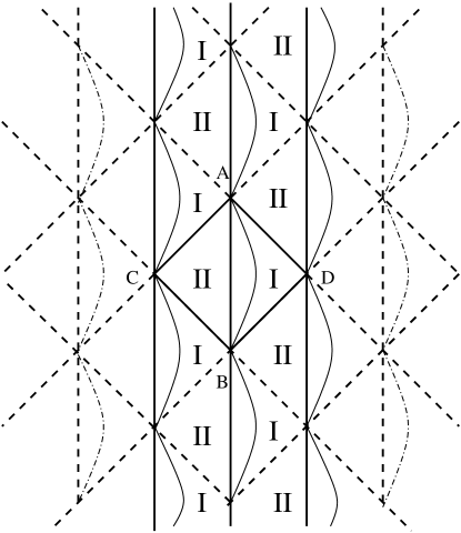
Figure 5: The Penrose diagram of the extended $AdS_{2}$ space. The vertical curves, both solid and dashed, represent hypersurfaces of constant $z>0$.

III.2 RS1 Model

To obtain the RS1 solution, we first make the coordinate transformation,

$${\ell}z=e^{\ell y},$$ (3.7)

so that metric (3.5) takes the form,

$$ds^{2}_{5}=e^{-2\ell y}\left(dt^{2}-d\Sigma^{2}_{0}\right)-dy^{2}.$$ (3.8)

Then, applying the replacement (2.8) in the above metric coefficients, we obtain the RS metric (1.1) with $y=r_{c}\phi$. Comparing it with the general form of the metric Eq.(2.9), we find

$$N\left(t,|y|\right) = A\left(t,|y|\right)=e^{-{\ell}|y|},$$

$$B\left(t,|y|\right) = 1,\;\;\;k=0.$$ (3.9)

Substituting Eq.(III.2) into Eqs.(II) and (II), we obtain

$$\rho_{0} = -p_{0}=\frac{1}{\kappa_{5}}\left(6{\ell}-\lambda_{0}\right),$$

$$\rho_{c} = -p_{c}=-\frac{1}{\kappa_{5}}\left(6{\ell}+\lambda_{c}\right).$$ (3.10)

RS chose

$$\lambda_{0}=-\lambda_{c}=6{\ell},$$ (3.11)

so that no matter fields appear on the two branes. In Fig. 4, the two 3-branes are represented by the two solid vertical curves with $z_{0}\equiv\ell^{-1}$ and $z_{c}\equiv\ell^{-1}e^{\ell y_{c}}$, respectively. The bulk is the region between these two curves, the shaded region. As shown in the last sub-section, the spacetime is not geodesically complete, and extension is needed. One possible extension is that given by Fig. 5 but with two vertical curves, one is $z=z_{0}$ and the other is $z=z_{c}$, where the bulk is the region between the two curves. Clearly, in this extension we have infinite number of RS1 universes.

III.3 Dynamical 3-branes in $AdS_{5}$

To find new solutions, we first make the coordinate transformation,

$$t = F\left(t^{\prime}+f(y^{\prime})\right)+G\left(t^{\prime}-f(y^{\prime})\right),$$

$$z = F\left(t^{\prime}+f(y^{\prime})\right)-G\left(t^{\prime}-f(y^{\prime})\right),$$ (3.12)

so that metric (3.5) takes the form,

$$ds^{2}_{5}=\frac{4F^{\prime}G^{\prime}}{{\ell}^{2}(F-G)^{2}}\left(d{t}^{2}-{f^{\prime}}^{2}(y)d{y}^{2}\right)-\frac{1}{{\ell}^{2}(F-G)^{2}}d\Sigma_{0}^{2},$$ (3.13)

where $F,\;G$ and $f$ are arbitrary functions, and a prime denotes ordinary differentiation with respect to their indicated arguments. Note that in writing Eq.(3.13), we had dropped the primes from $t^{\prime}$ and $y^{\prime}$. Replacing $y$ by $|y|$ in the metric coefficients, the resulting metric finally takes the form of Eq.(2.9), but now with

$$N(t,|y|) = \frac{2\sqrt{F^{\prime}G^{\prime}}}{{\ell}(F-G)},$$

$$B(t,|y|) = \frac{2\sqrt{F^{\prime}G^{\prime}}}{{\ell}(F-G)}{f^{\prime}}(|y|),$$

$$A(t,|y|) = \frac{1}{{\ell}(F-G)},$$ (3.14)

where

$$F=F\left(t+f(|y|)\right),\;\;\;G=G\left(t-f(|y|)\right),$$ (3.15)

and $|y|$ is given by Eq.(2.10). On the hypersurface $y=0$, the metric reduces to

$$\left.ds^{2}_{5}\right|_{y=0}=d\eta^{2}-a^{2}_{0}(\eta)d\Sigma_{0}^{2},$$ (3.16)

with

$$d\eta \equiv \frac{2\sqrt{{F^{\prime}}_{0}{G^{\prime}}_{0}}}{{\ell}(F_{0}-G_{0})}dt,$$

$$F_{0} \equiv F(t+f(0)),\;\;\;G_{0}\equiv G(t-f(0)),$$

$$a_{0}(\eta) \equiv \frac{1}{{\ell}(F_{0}-G_{0})},\;\;\;b_{0}(\eta)\equiv\frac{1}{{\ell}(F_{0}+G_{0})}.$$ (3.17)

From the above expressions it can be shown that

$$\left.\frac{{F^{\prime}}}{\sqrt{{F^{\prime}}{G^{\prime}}}}\right|_{y=0} = -\frac{a_{0}}{{\ell}}\left(\frac{\dot{b}_{0}}{b_{0}^{2}}+\frac{\dot{a}_{0}}{a_{0}^{2}}\right),$$

$$\left.\frac{{G^{\prime}}}{\sqrt{{F^{\prime}}{G^{\prime}}}}\right|_{y=0} = -\frac{a_{0}}{{\ell}}\left(\frac{\dot{b}_{0}}{b_{0}^{2}}-\frac{\dot{a}_{0}}{a_{0}^{2}}\right),$$ (3.18)

from which we find that

$$\frac{\dot{b}_{0}}{b_{0}^{2}} = \frac{\epsilon_{0}}{a_{0}}\left(\ell^{2}+H^{2}_{0}\right)^{1/2},$$

$$H_{0} \equiv \frac{\dot{a}_{0}}{a_{0}},\;\;\;\epsilon_{0}=\pm 1,$$ (3.19)

where $\dot{a}_{0}\equiv da_{0}/d\eta$. Inserting the above expressions into Eq.(III.3) we find that, in order for ${F^{\prime}}_{0}$ and ${G^{\prime}}_{0}$ to be real, $\epsilon_{0}$ must be chosen such that,

$$\epsilon_{0}=\cases{-1,&${F^{\prime}}_{0}>0,\;{G^{\prime}}_{0}>0$,\cr+1,&${F^{\prime}}_{0}<0,\;{G^{\prime}}_{0}<0$.\cr}$$ (3.20)

Substituting Eqs.(III.3) - (3.20) into Eq.(II) we obtain

$$\left(H_{0}^{2}+\ell^{2}\right)^{1/2} = -\frac{1}{6}\kappa_{5}\epsilon_{0}\epsilon^{0}_{f}\left({\rho}_{0}+\bar{\lambda}_{0}\right),$$ (3.21)

$$\frac{\dot{H}_{0}}{\left(H_{0}^{2}+\ell^{2}\right)^{1/2}} = \frac{1}{2}\kappa_{5}\epsilon_{0}\epsilon^{0}_{f}\left({\rho}_{0}+{p}_{0}\right),$$ (3.22)

where $\bar{\lambda}_{0}\equiv\lambda_{0}/\kappa_{5}$, and $\epsilon^{0}_{f}\equiv f^{\prime}(0)/\left|f^{\prime}(0)\right|$.

Similarly, on the TeV brane $y=y_{c}$, introducing the quantities,

$$d\tau \equiv \frac{2\sqrt{{F^{\prime}}_{c}{G^{\prime}}_{c}}}{{\ell}(F_{c}-G_{c})}dt,$$

$$F_{c} \equiv F\left(t+f(|y_{c}|)\right),\;\;\;G_{c}\equiv G\left(t-f(|y_{c}|\right),$$

$$a_{c}(\tau) \equiv \frac{1}{{\ell}(F_{c}-G_{c})},\;\;\;b_{c}(\tau)\equiv\frac{1}{{\ell}(F_{c}+G_{c})},$$ (3.23)

we find

$$\frac{\dot{b}_{c}}{b_{c}^{2}} = \frac{\epsilon_{c}}{a_{c}}\left(\ell^{2}+H^{2}_{c}\right)^{1/2},$$

$$H_{c} \equiv \frac{\dot{a}_{c}}{a_{c}},\;\;\;\epsilon_{c}=\pm 1.$$ (3.24)

Eq.(II) can be written as

$$\left(H_{c}^{2}+\ell^{2}\right)^{1/2} = \frac{1}{6}\kappa_{5}\epsilon_{c}\epsilon^{c}_{f}\left({\rho}_{c}+\bar{\lambda}_{c}\right),$$ (3.25)

$$\frac{\dot{H}_{c}}{\left(H_{c}^{2}+\ell^{2}\right)^{1/2}} = -\frac{1}{2}\kappa_{5}\epsilon_{c}\epsilon^{c}_{f}\left({\rho}_{c}+{p}_{c}\right),$$ (3.26)

where $\dot{H}_{c}\equiv dH_{c}/d\tau,\;\epsilon^{c}_{f}=f^{\prime}(y_{c})/|f^{\prime}(y_{c})|$, $\bar{\lambda}_{c}\equiv\lambda_{c}/\kappa_{5}$, and

$$\epsilon_{c}=\cases{-1,&${F^{\prime}}_{c}>0,\;{G^{\prime}}_{c}>0$,\cr+1,&${F^{\prime}}_{c}<0,\;{G^{\prime}}_{c}<0$.\cr}$$ (3.27)

Note that, in order to have $\rho_{c}\geq 0$ for any given $\bar{\lambda}_{c}$, we must choose $\epsilon_{c}$ and $\epsilon^{c}_{f}$ such that

$$\epsilon_{c}\epsilon^{c}_{f}=1,$$ (3.28)

a choice that we shall assume in the following discussions. To study the above system of differential equations further, let us consider the case where

$${\lambda}_{c}=0,\;\;\;p_{c}=w{\rho}_{c},$$ (3.29)

with $w$ being an arbitrary constant.

III.3.1 $w>-1$

In this case, Eqs.(3.25) and (3.26) have the general solution,

$$a_{c}(\tau) = C_{0}\sin\left[3{\ell}(1+w)\tau\right]^{\frac{1}{3(1+w)}},$$

$$\rho_{c}(\tau) = \frac{6{\ell}}{\kappa_{5}\sin\left[3{\ell}(1+w)\tau\right]},$$ (3.30)

where $C_{0}$ is a positive constant. From the above expressions we can see that in this case the universe starts to expand from a big-bang like singularity at $\tau=0$, until the moment $\tau_{max}\equiv\pi/[6{\ell}(1+w)]$. From that moment on the universe starts to contract until the moment $\tau_{f}\equiv\pi/[2{\ell}(1+w)]$, where the whole universe is crushed into a spacetime singularity.

For $-1<w<-2/3$ the universe experiences an accelerating period. In fact, from Eq.(III.3.1) we find that

$$\ddot{a}_{c}(\tau)=-C_{0}{\ell}^{2}\frac{(2+3w)+\sin^{2}\left[3{\ell}(1+w)\tau\right]}{\sin^{\frac{6w+5}{3(1+w)}}\left[3{\ell}(1+w)\tau\right]},$$ (3.31)

from which we can see that the universe is accelerating during the time $\tau_{0}<\tau<\pi-\tau_{0}$ for $w<-2/3$, where

$$\tau_{0}\equiv\frac{1}{3{\ell}(1-|w|)}{\mbox{Arcsin}}\left(\sqrt{3|w|-2}\right).$$ (3.32)

To study the global properties of the solutions, we first notice that

$$t_{c}(t) = F_{c}(t)+G_{c}(t)=\frac{1}{\ell b_{c}},$$

$$z_{c}(t) = F_{c}(t)-G_{c}(t)=\frac{1}{\ell a_{c}}$$ (3.33)

$$= \frac{1}{\ell C_{0}}\sin\left[{\ell}(1+w)\tau\right]^{-1/[3(1+w)]},$$

as we can see from Eqs.(III.3) and (III.3). Then, we find

$$\frac{dz_{c}}{dt_{c}}=\epsilon_{c}\cos\left[3(1+w)\ell\tau\right].$$ (3.34)

From Eqs.(III.3.1) and (3.34) we obtain

$$\epsilon_{c}t_{c}=\cases{\infty,&$\tau=0$,\cr 0,&$\tau=\tau_{max}$,\cr-\infty,&$\tau=\tau_{f}$.\cr}$$ (3.35)

In Fig. 6 the vertical line $GPH$ represents the visible 3-brane located at $y=y_{c}$. For $\epsilon_{c}=-1$, the 3-brane starts to expand from the initial moment $\tau=0$, denoted by the point $G$ in the figure, which is singular and corresponds to ($t_{c},z_{c})_{G}=(-\infty,\infty)$ in the ($t,z$)-plane [cf. Fig. 4]. The expansion is continuous until the moment $\tau=\tau_{max}$, where ($t_{c},z_{c})_{P}=(0,z_{c}^{min}$), with $z_{c}^{min}\equiv 1/(\ell C_{0})$. Afterward, the universe starts to collapse and a spacetime singularity of the 3-brane is finally formed at the moment $\tau_{f}$, where ($t_{c},z_{c})_{H}=(\infty,\infty$). The proper time of this whole process is finite and given by $\tau_{f}$. It should be noted that, unlike the RS1 solution, the extension beyond the two points $G$ and $H$ are not needed because now they are spacetime singularities of the 3-brane. It is also interesting to note that the five-dimensional bulk is not singular at all even at the points $G$ and $H$.

For $\epsilon_{c}=+1$, the evolution of the visible 3-brane follows the same curve $GPH$, but now the whole process is inverse in the ($t,z$)-plane. That is, the visible 3-brane starts to expand from the singular point $H$ until its maximal point $P$, and then collapses into a spacetime singularity at the point $G$.

Figure 6: The Penrose diagram for the case $w>-1$ of the solutions (III.3.1) in the ($t,z$)-plane of the horospheric coordinates, defined by Eq.(III.1). The evolution of the visible 3-brane, located on the hypersurface $y=y_{c}$, is denoted by the vertical curve $GPH$, and the evolution of the invisible 3-brane, located at $y=0$, is given by the dotted curve $GP^{\prime}H$. The five-dimensional bulk is the region between the two vertical curves. The spacetimes of the 3-branes are singular at the points $G$ and $H$, but not the bulk.

Repeating the above analysis for the invisible 3-brane at $y=0$, it is not difficult to see that its trajectory in the ($t,\;z$)-plane of the horospherical coordinates is the dotted curve $GP^{\prime}H$ in Fig. 6. So, the whole bulk is the region between the two curves $GP^{\prime}H$ and $GPH$.

III.3.2 $w=-1$

In this case, we have

$$a_{c}(\tau) = C_{0}e^{H_{c}\tau},$$

$$\rho_{c}(\tau) = -p_{c}=\frac{6}{\kappa_{5}}\left(H_{c}^{2}+{\ell}^{2}\right)^{1/2},$$ (3.36)

where now $H_{c}$ is a constant. Clearly, in the present case the universe is a de Sitter space, which is expanding exponentially. Inserting Eq.(III.3.2) into Eq.(III.3) and then integrating the resulting expression, we find

$$b_{c}(\tau)=\epsilon_{c}\frac{C_{0}H_{c}}{\left(H^{2}_{c}+\ell^{2}\right)^{1/2}}e^{H_{c}\tau}.$$ (3.37)

Thus, we obtain

$$\frac{z_{c}}{t_{c}} = \epsilon_{c}\frac{H_{c}}{\left(H^{2}_{c}+\ell^{2}\right)^{1/2}},$$

$$z_{c} = \frac{1}{\ell C_{0}}e^{-H_{c}\tau}$$

$$= \cases{\infty,&$\tau-\infty$,\cr 0,&$\tau+\infty$,\cr}$$

$$\epsilon_{c}t_{c} = \frac{\left(H^{2}_{c}+\ell^{2}\right)^{1/2}}{C_{0}H_{c}}e^{-H_{c}\tau}$$ (3.38)

$$= \cases{\infty,&$\tau-\infty$,\cr 0,&$\tau+\infty$.\cr}$$

Fig. 7 shows the trajectory of the visible 3-brane in the plane of the horospheric coordinates $t$ and $z$ for $\epsilon_{c}=-1$. The 3-brane starts from the moment $\tau=-\infty$ or $(t_{c},z_{c})=(-\infty,\infty)$, denoted by the point $B$ in the figure, and ends at $\tau=\infty$, where $(t_{c},z_{c})=(0,0)$, as shown by the vertical solid curve $BO$.

Figure 7: The Penrose diagram for the case $w=-1$ and $\epsilon_{c}=-1$ of the solution (III.3.2) in the ($t,z$)-plane of the horospheric coordinates, defined by Eq.(III.1). The evolution of the visible 3-brane, located on the hypersurface $y=y_{c}$, is denoted by the vertical curve $O^{\prime}BO$, and the trajectory of the invisible brane, located at $y=0$, is given by the dotted curve $O^{\prime}BO$. The five-dimensional bulk is the region between the two vertical curves. From the point of view of observers who live on the brane, these trajectories are geodesically complete and no extension is needed. But, from the point of view of “observers” in the five-dimensional bulk, the five-dimensional spacetime is not geodesically complete, and extension is needed. A possible extension is given by Fig. 8.

It should be noted that the spacetime described by the metric

$$ds^{2}_{4}=d\tau^{2}-C^{2}_{0}e^{2H_{c}\tau}d\Sigma_{0}^{2},$$ (3.39)

is not geodesically complete. As a matter of fact, it covers only half of the hyperboloid HE73 ,

$$-V^{2}+W^{2}+X^{2}+Y^{2}+Z^{2}=H^{-2}_{c},$$ (3.40)

with

$$V+W=H^{-1}_{c}e^{H_{c}\tau}>0.$$ (3.41)

To extend the spacetime to the other half of the hyperboloid, we introduce the coordinates $\hat{\tau}$ and $\chi$ via the relations,

$$\tau = H^{-1}_{c}\ln\left[H_{c}\left(V+W\right)\right],$$

$$r = \frac{1}{C_{0}H^{2}_{c}(V+W)}\cosh\left(H_{c}\hat{\tau}\right)\sin\chi,$$ (3.42)

where

$$V+W=\frac{1}{H_{c}}\left[\sinh\left(H_{c}\hat{\tau}\right)+\cosh\left(H_{c}\hat{\tau}\right)\cos\chi\right].$$ (3.43)

Then, we find that the metric (3.39) becomes

$$ds^{2}_{4}=d\hat{\tau}^{2}-H^{-2}_{c}\cosh^{2}\left(H_{c}\hat{\tau}\right)\left(d\chi^{2}+\sin^{2}\chi d\Sigma_{0}^{2}\right),$$ (3.44)

which covers the whole hyperboloid for $-\infty<\hat{\tau}<\infty$, $\;0\leq\chi,\;\theta\leq\pi$, and $0\leq\phi\leq 2\pi$.

On the other hand, from Eqs.(III.3.2) and (III.3.2) we find

$$z_{c} = \frac{1}{\ell C_{0}H_{c}\left(V+W\right)},$$

$$t_{c} = \frac{\epsilon_{c}\left(H^{2}_{c}+\ell^{2}\right)^{1/2}}{\ell C_{0}H_{c}^{2}\left(V+W\right)}.$$ (3.45)

Thus, across the surface $V+W=0$, both $z_{c}$ and $t_{c}$ change their signs. Then, the extended region must be the one given by the vertical dashed curve $O^{\prime}B$ in Fig. 7. Therefore, in the present case the geodesically complete spacetime of the visible 3-brane, described by metric (3.44), is that of the segment $O^{\prime}BO$.

However, as shown at beginning of this section, the spacetime described by metric (3.5) is not geodesically complete, and one possible extension is that given by Fig. 5. Clearly, in the present case, the five-dimensional bulk described by the solutions of Eqs.(III.3) and (III.3.2) is also not geodesically complete. A possible extension is given by Fig. 8. It is interesting to note that the segment $O^{\prime}BO$ is geodesically complete from the point of view of observers who live on the visible 3-brane, but this is no longer true from the point of view of the five-dimensional bulk. For the latter, the geodesically complete bulk is that given by Fig. 8, in which we have infinite number of geodesically complete visible 3-branes.

Figure 8: The Penrose diagram of the extended spacetime for $w=-1$ and $\epsilon_{c}=-1$, given by Eq.(III.3.2). The vertical curves, both solid and dashed, represent the history of a visible 3-brane. Each segment, consisting of a solid and a dashed part, is geodesically complete for observers living on the visible brane. The trajectory of the invisible 3-brane is represented by similar vertical curves, and the five-dimensional bulk is the region between the two curves, as shown in Fig. 7.

When $\epsilon_{c}=+1$, the global properties of the corresponding solution can be obtained from the case of $\epsilon_{c}=-1$ by the replacement $t_{c}\rightarrow-t_{c}$.

Similarly, it can be shown that the trajectory of the invisible brane located at $y=0$ is similar to that of the visible brane, and is given by the dotted curve $O^{\prime}BO$ in Fig. 7. The five-dimensional bulk is the region between the two vertical curves.

III.3.3 $w<-1$

In this case, we have

$$a_{c}(\tau) = \frac{C_{0}}{\sin\left[3{\ell}\left(\left|w\right|-1\right)\tau\right]^{\frac{1}{3(|w|-1)}}},$$

$$\rho_{c}(\tau) = \frac{6{\ell}}{\kappa_{5}\sin\left[3{\ell}(|w|-1)\tau\right]},$$ (3.46)

from which we can see that the universe is singular at $\tau=0$, where the radius of the universe is infinitely large $a_{c}(0)=\infty$. As time increases, the radius of the universe decreases until the moment $\tau=\tau_{min}$ when it reaches its minimum $a_{c}(\tau_{min})=a_{c}^{0}$, where

$$\tau_{min}\equiv\frac{\pi}{6{\ell}(|w|-1)}.$$ (3.47)

After this moment, the radius of the universe starts to increase until the moment $\tau=2\tau_{min}$, at which it becomes infinitely large, and the spacetime becomes singular. Note that in this case the acceleration is always positive,

$$\ddot{a}_{c}(\tau)=C_{0}{\ell}^{2}\frac{3(|w|-1)+\cos^{2}\left[3{\ell}(|w|-1)\tau\right]}{\sin^{\frac{6|w|-5}{3(|w|-1)}}\left[3{\ell}(|w|-1)\tau\right]}.$$ (3.48)

On the other hand, we have

$$\frac{dz_{c}}{dt_{c}} = -\epsilon_{c}\cos\left[3(|w|-1)\ell\tau\right],$$

$$z_{c}(t) = \frac{1}{\ell C_{0}}\sin\left[3{\ell}(|w|-1)\tau\right]^{1/[3(|w|-1)]}$$ (3.49)

$$= \cases{0,&$\tau=0$,\cr(\ell C^{0})^{-1},&$\tau=\tau_{min}$,\cr 0,&$\tau=2\tau_{min}$.\cr}$$

Thus, in the $(t_{c},z_{c})$-plane of the horospherical coordinates, for the case $\epsilon_{c}=-1$ the visible 3-brane starts to collapse from the singular point $(t_{c},z_{c})=(0,0)$ until the point $z_{c}(\tau_{min})=(\ell C_{0})^{-1}$. Afterward, it starts to expand upto the moment $\tau=2\tau_{in}$, where $(t_{c},z_{c})=(t_{c}^{0},0)$, at which a spacetime singularity is developed [cf. Fig. 9]. Since the 3-brane is singular at the points $O$ and $P$, the spacetime of the visible 3-brane is not extendible beyond these two points.

The global properties for the case of $\epsilon_{c}=+1$ can be obtained from the one of $\epsilon_{c}=-1$ by the replacement $t_{c}\rightarrow-t_{c}$.

Similarly, it can be shown that the trajectory of the invisible 3-brane is denoted by the dotted curve $OP$ in Fig. 9.

Figure 9: The Penrose diagram of the extended spacetime for $w<-1$ and $\epsilon_{c}=-1$ of the solutions (III.3.3) in the ($t,z$)-plane of the horospheric coordinates. The trajectory of the visible (invisible) 3-brane is denoted by the solid (dotted) curve $OP$. The spacetimes of the visible and invisible 3-branes are singular at the points $O$ and $P$.

IV Two 3-Branes in vacuum Bulk with $k=0$

When the bulk is vacuum and the spatial sectors of the two 3-branes are flat, $k=0$, the corresponding solutions of the five-dimensional bulk are well-known Taub51 ; BCG00 , and they can be divided into three different classes, which will be referred to, respectively, as Class IA, Class IB, and Class II solutions. In the following we consider them separately.

IV.1 Class IA Solutions

This class of solutions, after the replacement of Eq.(2.8), is given by

$$N^{2}(t,|y|) = \frac{FG^{\prime}}{G^{2/3}},$$

$$A^{2}(t,|y|) = G^{2/3},$$

$$B^{2}(t,|y|) = \frac{FG^{\prime}}{G^{2/3}}{f^{\prime}(|y|)}^{2},$$ (4.1)

where $F$ and $G$ are given by Eq.(3.15), with $f(|y|)$ being arbitrary function of $|y|$ only. As first noticed by Taub Taub51 , the spacetime outside the 3-branes in this case is flat. In fact, introducing the coordinates $T$ and $X^{i}\;(i=1,2,3,4)$ via the relations,

$$T-X^{1} = G^{1/3}\left(t-f(y)\right),$$

$$T+X^{1} = 3\int^{t+f(y)}{F(x)dx}$$

$$+G^{1/3}\left(t-f(y)\right)\left[\left(x^{2}\right)^{2}+\left(x^{3}\right)^{2}+\left(x^{4}\right)^{2}\right],$$

$$X^{i} = G^{1/3}\left(t-f(y)\right)x^{i},\;(i=2,3,4),$$ (4.2)

the metric outside the 3-branes will take the Minkowski form, $ds^{2}_{5}=\eta_{AB}dX^{A}dX^{B}$. From the above expressions we find that

$$T^{2}-R^{2}=3G^{1/3}\left(t^{2}-f(y)\right)\int^{t+f(y)}{F(x)dx},$$ (4.3)

where $R^{2}\equiv\left(X^{1}\right)^{2}+\left(X^{2}\right)^{2}+\left(X^{3}\right)^{2}+\left(X^{4}\right)^{2}$.

Introducing $\tau$ and $a_{c}(\tau)$ via the relations,

$$d\tau=\left(\frac{F_{c}{G^{\prime}}_{c}}{{G}_{c}^{2/3}}\right)^{1/2}dt,$$

$$a_{c}(\tau)=G_{c}^{1/3}(t),$$ (4.4)

we find that Eq.(II) yields,

$$\frac{\dot{H}_{c}}{H_{c}} = \frac{1}{2}\kappa_{5}\epsilon_{c}\left(\rho_{c}+p_{c}\right),$$

$$H_{c} = -\frac{1}{6}\kappa_{5}\epsilon_{c}\left(\rho_{c}+\bar{\lambda}_{c}\right),$$ (4.5)

where, as previously, $H_{c}\equiv\dot{a}_{c}/a_{c}$, $\dot{H}_{c}\equiv dH_{c}/d\tau$, and $\epsilon_{c}\equiv f^{\prime}(|y_{c}|)/|f^{\prime}(|y_{c}|)|$. It is remarkable to note that $F_{c}(t)$ does not appear explicitly in Eq.(IV.1).

When $\lambda_{c}=0$ and $p_{c}=w\rho_{c}$, Eq.(IV.1) has the solution,

$$a_{c}(\tau)=\tau^{\frac{1}{3(1+w)}},$$ (4.6)

from which we find that

$$\ddot{a}_{c}(\tau) = -\frac{3w+2}{9(1+w)^{2}}\tau^{-\frac{6w+5}{3(1+w)}},$$

$$\rho_{c}(\tau) = -\frac{2\epsilon_{c}}{\kappa_{5}(1+w)\tau}.$$ (4.7)

Clearly, to have $\rho_{c}$ non-negative, we much choose $\epsilon_{c}$ such that

$$\epsilon_{c}=\cases{-1,&$w>-1$,\cr+1,&$w<-1$.\cr}$$ (4.8)

From Eq.(IV.1) we can also see that the universe is accelerating for $w<-2/3$.

It should be noted that Eqs.(4.6) and (IV.1) hold only for $w\not=-1$. When $w=-1$ from Eq.(IV.1) we find that

$$a_{c}(\tau) = a_{0}e^{H_{c}\tau},$$

$$\rho_{c}(\tau) = -p_{c}(\tau)=-\frac{6\epsilon_{c}H_{c}}{\kappa_{5}},\;(w=-1),$$ (4.9)

where $a_{0}$ and $H_{c}$ are positive constants. Obviously, the spacetime of the visible 3-branes is always acceleratingly expanding.

On the other hand, from Eq.(4.3) we find that the visible 3-brane in the five-dimensional Minkowski coordinates $T$ and $X^{i}$ is a hyperboloid,

$$\left[T^{2}-R^{2}\right]_{y=y_{c}} = 3G^{1/3}\left(t-f(y_{c})\right)$$ (4.10)

$$\times\int^{t+f(y_{c})}{F(x)dx}.$$

Similarly, the invisible 3-brane located at $y=0$ is also a hyperboloid,

$$\left[T^{2}-R^{2}\right]_{y=0} = 3G^{1/3}\left(t-f(0)\right)$$ (4.11)

$$\times\int^{t+f(0)}{F(x)dx}.$$

The two 3-branes will collide at the moment $t_{d}$, where $t_{d}$ is a solution of the equation,

$$\left[\frac{G\left(t-f(y_{c})\right)}{G\left(t-f(0)\right)}\right]^{1/3}=\frac{\int^{t+f(y_{c})}{F(x)dx}}{\int^{t+f(0)}{F(x)dx}}.$$ (4.12)

The bulk is the region between these two hyperboloids. However, since it is flat, no radiation, neither gravitational nor non-gravitational, from the two 3-branes is leaked into the bulk, although there may be energy exchange between the two 3-branes at the moment when they collide [cf. Fig. 10].

Figure 10: The two 3-branes in the Minkowski coordinates $T$ and $X^{i}\;(i=1,2,3,4)$, defined by Eq.(IV.1), at a given time $t$. Each of the two branes is a hyperboloid. In some cases the two branes collide, provided that Eq.(4.12) has real solutions.

IV.2 Class IB Solutions

In this case, the solutions are given by

$$N^{2}(t,|y|) = \frac{F^{\prime}G}{F^{2/3}},$$

$$A^{2}(t,|y|) = F^{2/3},$$

$$B^{2}(t,|y|) = \frac{F^{\prime}G}{F^{2/3}}{f^{\prime}(|y|)}^{2}.$$ (4.13)

Introducing $\tau$ and $a_{c}(\tau)$ via the relations,

$$d\tau=\left(\frac{{F^{\prime}}_{c}G_{c}}{{F}_{c}^{2/3}}\right)^{1/2}dt,$$

$$a_{c}(\tau)=F_{c}^{1/3}(t),$$ (4.14)

we find that Eq.(II) yields,

$$\frac{\dot{H}_{c}}{H_{c}} = -\frac{1}{2}\kappa_{5}\epsilon_{c}\left(\rho_{c}+p_{c}\right),$$

$$H_{c} = \frac{1}{6}\kappa_{5}\epsilon_{c}\left(\rho_{c}+\bar{\lambda}_{c}\right).$$ (4.15)

Comparing Eq.(IV.2) with Eq.(IV.1) we can see that we can obtain one from the other by simply replacing $\epsilon_{c}$ by $-\epsilon_{c}$. Thus, the physics of the solutions in the present case can be deduced from the ones given in the last case. Therefore, in the following we shall not consider this case any further.

IV.3 Class II Solutions

In this case, the corresponding solutions are given by

$$N^{2}(t,|y|) = \frac{F^{\prime}G^{\prime}}{\left(F+G\right)^{2/3}},$$

$$A^{2}(t,|y|) = \left(F+G\right)^{2/3},$$

$$B^{2}(t,|y|) = \frac{F^{\prime}G^{\prime}}{\left(F+G\right)^{2/3}}{f^{\prime}(|y|)}^{2}.$$ (4.16)

Before studying the dynamics of the 3-branes, let us first consider the global structure of the spacetime described by the above solutions without 3-branes, that is, the solutions of Eq.(IV.3) with $|y|$ being replaced by $y$ where we temporarily extend the range of $y$ to $y\in(-\infty,\infty)$. Then, by the coordinate transformation,

$$T\equiv F+G,\;\;\;Y\equiv F-G,$$ (4.17)

the corresponding metric takes the form,

$$ds^{2}_{5}=\frac{1}{4T^{2/3}}\left(dT^{2}-dY^{2}\right)-T^{2/3}d\Sigma^{2}_{0}.$$ (4.18)

Clearly, the 5D spacetime is singular at $T=0$, and the corresponding Penrose diagram is given by Fig. 11.

Figure 11: The Penrose diagram of the solutions of Eq.(4.18) in the $(T,Y)$-plane, defined by Eq.(4.17). The five-dimensional spacetime is singular at $T=0$.

Introducing $\tau$, $a_{c}(\tau)$ and $b_{c}(\tau)$ via the relations,

$$d\tau=\left(\frac{{F^{\prime}}_{c}{G^{\prime}}_{c}}{\left(F_{c}+{G}_{c}\right)^{2/3}}\right)^{1/2}dt,$$

$$a_{c}(\tau)=\left(F_{c}+{G}_{c}\right)^{1/3},$$

$$b_{c}(\tau)=\left(F_{c}-{G}_{c}\right)^{1/3},$$ (4.19)

from Eq.(II) we find,

$$\frac{\dot{H}_{c}+2\left(H^{2}_{c}-\Delta^{2}\right)}{\Delta} = -\frac{1}{2}\kappa_{5}\epsilon_{c}^{0}\epsilon_{c}\left(\rho_{c}+p_{c}\right),$$

$$\Delta = \frac{1}{6}\kappa_{5}\epsilon_{c}^{0}\epsilon_{c}\left(\rho_{c}+\bar{\lambda}_{c}\right),$$ (4.20)

where $\epsilon_{c}^{0}=\pm 1$, and

$$\Delta\equiv\left(H^{2}_{c}-\frac{4}{9a^{4}_{c}}\right)^{1/2},$$

$$\dot{b}_{c}(\tau)=\frac{\epsilon_{c}^{0}a^{3}_{c}}{b^{2}_{c}}\Delta.$$ (4.21)

To study this case further, in the rest of this sub-section, we also restrict ourselves to the case where $\lambda_{c}=0$ and $p_{c}=w\rho_{c}$. Then, from Eq.(IV.3) we find that

$$\ddot{a}_{c}+(2+3w)\frac{\dot{a}_{c}^{2}}{a_{c}}-\frac{4(1+3w)}{9a^{3}_{c}}=0.$$ (4.22)

To solve this equation, it is found convenient to distinguish the following cases.

IV.3.1 $w>-\frac{1}{3}$

In this case, introducing the function $X(\tau)$ via the relation

$$a_{c}(\tau)=\beta X^{\frac{1}{3(1+w)}},$$ (4.23)

where $\beta$ is an arbitrary constant and different from the one introduced in Eq.(2.5), Eq.(4.22) reduces to,

$$\ddot{X}-\frac{4(1+w)(1+3w)}{3\beta^{4}}X^{\frac{3w-1}{3(1+w)}}=0.$$ (4.24)

Choosing the constant $\beta$ as

$$\beta=\left|\frac{4(1+w)(1+3w)}{3}\right|^{1/4},$$ (4.25)

we find that Eq.(4.24) finally takes the form

$$\ddot{X}-X^{-\delta}=0,$$ (4.26)

where

$$\delta\equiv\frac{1-3w}{3(1+w)}.$$ (4.27)

It can be shown that Eq.(4.26) allows the first integral,

$$\dot{X}=\pm\sqrt{\frac{X^{2n}+X_{1}}{n}},$$ (4.28)

where $X_{1}$ is an integration constant, and

$$n\equiv\frac{1-\delta}{2}=\frac{1+3w}{3(1+w)},$$ (4.29)

from which we find that for $-1/3<w<\infty$ we always have $0<n\leq 1$. To have an expanding universe, in the following we shall choose the “+” sign in Eq.(4.28).

When $w=\frac{1}{3}$, Eq.(4.28) can be integrated explicitly and gives,

$$a_{c}(\tau) = \sqrt{\frac{4}{3}}\left\{\left(\tau+\tau_{0}\right)^{2}-\tau^{2}_{0}\right\}^{1/4},$$

$$\dot{a}_{c}(\tau) = \frac{\tau+\tau_{0}}{\sqrt{3}\left[\left(\tau+\tau_{0}\right)^{2}-\tau^{2}_{0}\right]^{3/4}},$$

$$\ddot{a}_{c}(\tau) = -\frac{\left(\tau+\tau_{0}\right)^{2}+2\tau^{2}_{0}}{\sqrt{12}\left[\left(\tau+\tau_{0}\right)^{2}-\tau^{2}_{0}\right]^{7/4}},$$

$$\rho_{c}(\tau) = \frac{3\epsilon^{0}_{c}\epsilon_{c}\tau_{0}}{\kappa_{5}\left[\left(\tau+\tau_{0}\right)^{2}-\tau^{2}_{0}\right]},\;(w=1/3),$$ (4.30)

where $\tau_{0}$ is a constant. Clearly, in this case the universe starts to expand from the singular point $\tau=0$, and the acceleration of the expansion is always negative.

On the other hand, from Eqs.(4.17), (IV.3) and (IV.3.1) we find that

$$Y_{c}(\tau) = \frac{3\epsilon^{0}_{c}\tau_{0}}{2}\left(\frac{4}{3}\right)^{3/2}\int{\frac{d\tau}{\left[(\tau+\tau_{0})^{2}-\tau^{2}_{0}\right]^{1/4}}},$$

$$T_{c}(\tau) = \left(\frac{4}{3}\right)^{3/2}\left[(\tau+\tau_{0})^{2}-\tau^{2}_{0}\right]^{3/4}.$$ (4.31)

Thus, we have $T_{c}(0)=Y_{c}(0)=0$, and

$$T_{c}(\tau) \sim \tau^{3/2}\rightarrow\infty,$$

$$Y_{c}(\tau) \sim \tau^{1/2}\rightarrow\infty,$$ (4.32)

as $\tau\rightarrow\infty$. Then, one can see that the trajectory of the visible 3-brane in the $(T,Y)$-plane is given by the solid curve $OAP$ for $\epsilon^{0}_{c}=+1$ and $OBP$ for $\epsilon^{0}_{c}=-1$, respectively, in Fig. 12.

Similarly, it can be shown that the trajectory of the invisible 3-brane in the $(T,Y)$-plane is given by the dotted curve $OA^{\prime}P$ for $\epsilon^{0}_{c}=+1$ and $OB^{\prime}P$ for $\epsilon^{0}_{c}=-1$ in Fig. 12. Then, the five-dimensional bulk is the region between the solid and dotted curves in each case. The spacetimes of both visible and invisible 3-branes are singular at the initial moment $\tau=0$.

Figure 12: The Penrose diagram of the Class II solutions in the $(T,Y)$-plane for $w>-1$. The solid (dotted) curves $OAP$ ($OA^{\prime}P$) and $OBP$ ($OB^{\prime}P$) are the trajectories of the visible (invisible) 3-branes, respectively, for $\epsilon^{0}_{c}=+1$ and $\epsilon^{0}_{c}=-1$. The spacetimes of both visible and invisible 3-branes are singular at the point $O$.

When $w\not=\frac{1}{3}$, using the integral,

$$\int{\frac{dx}{\sqrt{x^{2n}+a^{2n}}}}=\frac{x}{a^{n}}F\left(\frac{1}{2},\frac{1}{2n};1+\frac{1}{2n};-\left(\frac{x}{a}\right)^{2n}\right),$$

we find that Eq.(4.28) has the solution,

$$X\;F\left(\frac{1}{2},\frac{1}{2n};1+\frac{1}{2n};-\left(\frac{X}{X_{0}}\right)^{2n}\right)=\left(\frac{X^{2n}_{0}}{n}\right)^{1/2}\tau,$$ (4.34)

where $X_{0}=X^{1/2n}_{1}$, and $F(a,b;c;z)$ denotes the ordinary hypergeometric function with

$$F(a,b;c;0)=1.$$ (4.35)

Then, from Eqs.(4.23), (4.34) and (4.35), we find

$$a_{c}(\tau=0)=0.$$ (4.36)

On the other hand, using the relation,

$$F(a,b;c;z) = \frac{\Gamma(c)\Gamma(b-a)}{\Gamma(b)\Gamma(c-a)}(-z)^{-a}$$

$$\times F\left(a,1-c+a;1-b+a;\frac{1}{z}\right)$$

$$+\frac{\Gamma(c)\Gamma(a-b)}{\Gamma(a)\Gamma(c-b)}(-z)^{-b}$$

$$\times F\left(b,1-c+b;1-a+b;\frac{1}{z}\right),$$

we find

$$X\;F\left(\frac{1}{2},\frac{1}{2n};1+\frac{1}{2n};-\left(\frac{X}{X_{0}}\right)^{2n}\right) \simeq \frac{X^{n}_{0}}{1-n}X^{1-n}$$ (4.38)

$$\rightarrow\infty,$$

as $X\rightarrow\infty$. Therefore, we must have

$$a_{c}(\tau=\infty)=\infty.$$ (4.39)

From the above expressions, we also find that

$$\ddot{a}_{c}(\tau) = -\frac{\beta}{3(1+w)(1+3w)}\left(X^{-\frac{1}{1+w}}\right.$$ (4.40)

$$\left.+(3w+2)X^{2n}_{0}X^{-\frac{6w+5}{3(1+w)}}\right).$$

Thus, in the present case the universe is always decelerating. It can also be shown that

$$\rho_{c}(\tau)=\frac{\rho_{0}}{X},$$

$$\rho_{0}\equiv\frac{6\epsilon^{0}_{c}\epsilon_{c}X^{n}_{0}}{\sqrt{3(1+w)(1+3w)\kappa^{2}_{5}}}.$$ (4.41)

From Eqs.(4.17), (IV.3) and (4.23), on the other hand, we find that

$$Y_{c}(\tau) = \epsilon_{c}^{0}\beta^{3}X^{1/(1+w)}$$

$$\times F\left(\frac{1}{2},\frac{3}{2(1+3w)};\frac{5+6w}{2(1+3w)};-\left(\frac{X}{X_{0}}\right)^{2n}\right),$$

$$T_{c}(\tau) = a^{3}_{c}(\tau)=\beta^{3}X^{1/(1+w)}.$$ (4.42)

Thus, we have $T_{c}(0)=Y_{c}(0)=0$, and

$$T_{c}(\tau) \sim X^{1/(1+w)}\rightarrow\infty,$$

$$Y_{c}(\tau) \sim \epsilon_{c}^{0}\beta^{3}\left(\frac{3X^{n}_{0}}{2-3w}X^{\frac{2-3w}{3(1+w)}}+C_{0}\right),$$ (4.43)

as $\tau\rightarrow\infty$ (or $X\rightarrow\infty$), where

$$C_{0}\equiv\frac{3X^{1/(1+w)}_{0}}{2(1+3w)\pi^{1/2}}\Gamma\left(\frac{3}{2(1+3w)}\right)\Gamma\left(\frac{3w-2}{2(1+3w)}\right).$$ (4.44)

Since $1/(1+w)>(2-3w)/[3(1+w)]$ for $w>-1/3$, we find that the trajectory of the visible 3-brane in the $(T,Y)$-plane is also given by the curves $OAP$ and $OBP$ in Fig. 12, respectively, for $\epsilon_{c}^{0}=1$ and $\epsilon_{c}^{0}=-1$. The trajectory of the invisible 3-brane at $y=0$ is similar to the visible 3-brane, as indicated by the dotted vertical curves.

IV.3.2 $w=-\frac{1}{3}$

In this case, Eq.(4.22) has the solution,

$$a_{c}(\tau)=a_{0}\tau^{1/2},\;(w=-1/3),$$ (4.45)

where $a_{0}$ is a positive constant. Then, the corresponding energy density is given by

$$\rho_{c}(\tau)=\frac{\rho^{0}_{c}}{\tau},$$

$$\rho_{c}^{0}\equiv\frac{3\epsilon^{0}_{c}\epsilon_{c}}{\kappa_{5}}\left(1-\frac{16}{9a_{0}^{4}}\right)^{1/2}.$$ (4.46)

It is interesting to note that choosing $a_{0}=\sqrt{3/4}$ we have $\rho_{c}=0$, and the spacetime on the 3-brane becomes vacuum.

To study the global structure of the 3-branes in this case, we first notice that

$$T_{c}(\tau)=a^{3}_{0}\tau^{3/2},$$

$$Y_{c}(\tau)=Y^{0}_{c}\tau^{3/2},$$

$$Y_{c}^{0}\equiv\epsilon^{0}_{c}a^{3}_{0}\left(1-\frac{16}{9a_{0}^{4}}\right)^{1/2}.$$ (4.47)

Since $\left|Y_{c}^{0}\right|<a^{3}_{0}$, it can be shown that the corresponding Penrose diagram for the visible and invisible 3-branes is also given by Fig. 12.

IV.3.3 $-1<w<-\frac{1}{3}$

In this case, choosing the constant $\beta$ as that given by Eq.(4.25), we find that Eq.(4.24) becomes

$$\ddot{X}+X^{-\delta}=0,$$ (4.48)

where $\delta$ is still given by Eq.(4.27). It can be shown that Eq.(4.48) has the first integral,

$$\dot{X}=\pm\sqrt{\frac{X^{-2m}+X_{1}}{m}},$$ (4.49)

where

$$m\equiv\frac{\delta-1}{2}=-\frac{1+3w}{3(1+w)}>0.$$ (4.50)

When $w=-\frac{2}{3}$, Eq.(4.49) has the solution,

$$a_{c}(\tau)=a_{0}\left[\tau\left(\tau+\frac{4}{3a^{2}_{0}}\right)\right]^{1/2},\;(w=-2/3),$$ (4.51)

where $a_{0}$ is a positive constant. Then, we find that

$$\dot{a}_{c}(\tau) = a_{0}\frac{\tau+\frac{2}{3a^{2}_{0}}}{\left[\tau\left(\tau+\frac{4}{3a^{2}_{0}}\right)\right]^{1/2}},$$

$$\ddot{a}_{c}(\tau) = -\frac{4}{9a^{3}_{0}\left[\tau\left(\tau+\frac{4}{3a^{2}_{0}}\right)\right]^{3/2}},$$

$$\rho_{c}(\tau) = \frac{6\epsilon^{0}_{c}\epsilon_{c}}{\kappa_{5}}\left[\tau\left(\tau+\frac{4}{3a^{2}_{0}}\right)\right]^{-1/2},$$ (4.52)

from which we can see that the universe starts to expand from the singular point $\tau=0$. In this case the acceleration of the expansion is always negative.

On the other hand, it can be shown that

$$T_{c}(\tau) = a^{3}_{0}\left[\tau\left(\tau+\frac{4}{3a^{2}_{0}}\right)\right]^{3/2},$$

$$Y_{c}(\tau) = \epsilon^{0}_{c}a^{3}_{0}\tau^{2}\left(\tau+\frac{2}{a^{2}_{0}}\right).$$ (4.53)

Then, we find that $T_{c}(\tau)-\left|Y_{c}(\tau)\right|\rightarrow+\infty$, as $\tau\rightarrow\infty$. Hence, the trajectories of the visible and invisible 3-branes in this case are also given by Fig. 12 in the ($T,Y$)-plane.

When $w\not=-\frac{2}{3}$, Eq.(4.49) has the solution,

$$X^{1+m}F\left(\frac{1}{2},\frac{1+m}{2m};\frac{1+3m}{2m};-\left(\frac{X}{X_{0}}\right)^{2m}\right)$$

$$\;\;\;\;\;=\frac{1+m}{\sqrt{m}}\tau,$$ (4.54)

where $X_{1}\equiv X^{-2m}_{0}$. Then, it can be shown that

$$X(\tau)=\cases{0,&$\tau=0$,\cr\infty,&$\tau\rightarrow\infty$,\cr}$$ (4.55)

and that

$$\rho_{c}(\tau) = \epsilon^{0}_{c}\epsilon_{c}\left(\frac{12X_{1}}{\kappa^{2}_{5}(1-|w|)(3|w|-1)}\right)^{1/2}\frac{1}{X},$$

$$\ddot{a}_{c}(\tau) = -\frac{\beta X^{\frac{6|w|-5}{3(1-|w|)}}}{3(1-|w|)(3|w|-1)}\left\{X^{-\frac{2(3|w|-1)}{3(1-|w|)}}\right.$$ (4.56)

$$-X_{1}\left(3|w|-2)\right\}.$$

Therefore, when $-1<w<-2/3$, there exists a moment, $\tau_{f}$, after which $\ddot{a}_{c}(\tau)$ becomes positive, that is, the universe turns to its accelerating phase from a decelerating one, where $\tau_{f}$ is the root of the equation,

$$X^{-\frac{2(3|w|-1)}{3(1-|w|)}}-X_{1}\left(3|w|-2\right)=0.$$ (4.57)

On the other hand, it can be shown that

$$Y_{c}(\tau) = \epsilon^{0}_{c}\frac{3\beta^{3}X_{1}^{1/2}}{2-3w}X^{\frac{2-3w}{3(1+w)}}$$

$$\times F\left(\frac{1}{2},\frac{3w-2}{2(1+3w)};\frac{9w}{2(1+3w)};-\left(\frac{X}{X_{0}}\right)^{2m}\right),$$

$$T_{c}(\tau) = \beta^{3}X^{\frac{1}{1+w}},$$ (4.58)

from which we find that $T_{c}(0)=0=Y_{c}(0)$, and

$$T_{c}(\tau) \sim X^{\frac{1}{1+w}}\rightarrow\infty,$$

$$\epsilon^{0}_{c}Y_{c}(\tau) \sim X^{\frac{2}{3(1+w)}}\rightarrow\infty,$$ (4.59)

as $X\rightarrow\infty$ (or $\tau\rightarrow\infty$). Following the arguments given above it can be shown that in this case the trajectories of the two 3-branes are given by Fig. 12, too.

IV.3.4 $w=-1$

In this case, introducing the function $X(\tau)$ via the relation

$$a_{c}=e^{X},$$ (4.60)

we find that Eq.(4.22) can be written as

$$\ddot{X}+\frac{8}{9}e^{-4X}=0,$$ (4.61)

which has the first integral,

$$\dot{X}=\pm\frac{2}{3}\sqrt{e^{-4X}+X_{0}},$$ (4.62)

where $X_{0}$ is an integration constant. When $X_{0}=0$ it can be shown that the corresponding solution represents a vacuum 3-brane ($\rho_{c}=0$), as that given by Eq.(4.45) with $a_{0}=\sqrt{3/4}$. When $X_{0}<0$ there are no real solutions. When $X_{0}>0$, Eq.(4.62) has the solution,

$$a_{c}(\tau)=a_{0}\sinh^{1/2}\left(\frac{4}{3a^{2}_{0}}\tau\right).$$ (4.63)

Then, we find that

$$\rho_{c}(\tau) = -p_{c}=\frac{4\epsilon^{0}_{c}\epsilon_{c}}{\kappa_{5}a^{2}_{0}},$$

$$\ddot{a}_{c}(\tau) = \frac{4}{9a^{3}_{0}\sinh^{3/2}\left(\frac{4}{3a^{2}_{0}}\tau\right)}$$ (4.64)

$$\times\left\{\sinh^{2}\left(\frac{4}{3a^{2}_{0}}\tau\right)-1\right\},$$

which shows that at the beginning the universe is decelerating, but after the moment $\tau=\tau_{f}$ it starts to accelerate, where $\tau_{f}$ is given by

$$\tau_{f}=\frac{3a^{2}_{0}}{4}\ln\left(1+\sqrt{2}\right).$$ (4.65)

It is interesting to note that in the present case we have $\rho_{c}=-p_{c}=Const.$

On the other hand, from Eqs.(4.17), (IV.3) and (4.63) we find that

$$Y_{c}(\tau) = 2\epsilon^{0}_{c}a_{0}\int{\sinh^{3/2}\left(\frac{4}{3a^{2}_{0}}\tau\right)d\tau},$$

$$T_{c}(\tau) = a_{0}^{3}\sinh^{3/2}\left(\frac{4}{3a^{2}_{0}}\tau\right).$$ (4.66)

Clearly, in this case we have $T_{c}(0)=0=Y_{c}(0)$, and $T_{c}(\tau)-\left|Y_{c}(\tau)\right|\rightarrow-\infty$, as $\tau\rightarrow\infty$. Then, the trajectory of the visible 3-brane in the ($T,Y$)-plane is given by the solid curve $OA$ for $\epsilon^{0}_{c}=+1$ and $OB$ for $\epsilon^{0}_{c}=-1$ in Fig. 13. Similarly, the trajectory of the invisible 3-brane is given by the dotted curves $OA$ and $OB$, respectively, for $\epsilon^{0}_{c}=+1$ and $\epsilon^{0}_{c}=-1$. The bulk is the region between the solid and dotted curves.

Figure 13: The Penrose diagram of the solutions of Eq.(4.63) in the $(T,Y)$-plane for $w=-1$. The solid (dotted) curves $OA$ and $OB$ are the trajectories of the visible (invisible) 3-branes, respectively, for $\epsilon^{0}_{c}=+1$ and $\epsilon^{0}_{c}=-1$.

IV.3.5 $w<-1$

In this case, choosing the constant $\beta$ as that given by Eq.(4.25), Eq.(4.24) becomes

$$\ddot{X}-X^{\delta}=0,$$ (4.67)

but now with

$$\delta\equiv\frac{1+3|w|}{3(|w|-1)}.$$ (4.68)

Eq.(4.67) has the first integral,

$$\dot{X}=\pm\sqrt{\frac{X^{2l}+X_{0}}{l}},$$ (4.69)

where

$$l\equiv\frac{3|w|-1}{3(|w|-1)}.$$ (4.70)

To have an expanding universe, now we must choose the “-” sign in Eq.(4.69). Then, Eq.(4.69) has the solution,

$$X\;F\left(\frac{1}{2},\frac{1}{2l};1+\frac{1}{2l};-\left(\frac{X}{X_{0}}\right)^{2l}\right)=\left(\frac{X^{2l}_{0}}{l}\right)^{1/2}\left(\tau_{s}-\tau\right),$$ (4.71)

where $X_{1}\equiv X_{0}^{2l}$, and

$$\tau_{s}\equiv\sqrt{\frac{l}{\pi}}X^{1-l}_{0}\Gamma\left(1+\frac{1}{2l}\right)\Gamma\left(\frac{1}{2}-\frac{1}{2l}\right).$$ (4.72)

From Eqs.(IV.3.1) and (4.71) we find

$$X(\tau)=\cases{0,&$\tau=\tau_{s}$,\cr\infty,&$\tau=0$,\cr}$$ (4.73)

and

$$a_{c}(\tau)=\beta X^{-\frac{1}{3(|w|-1)}}=\cases{\infty,&$\tau=\tau_{s}$,\cr 0,&$\tau=0$.\cr}$$ (4.74)

On the other hand, we also have

$$\rho_{c}(\tau) = \epsilon^{0}_{c}\epsilon_{c}\left(\frac{12X_{1}}{\kappa^{2}_{5}(|w|-1)(3|w|-1)}\right)^{1/2}\frac{1}{X},$$

$$\ddot{a}_{c}(\tau) = \frac{\beta X^{-\frac{6|w|-5}{3(|w|-1)}}}{3(|w|-1)(3|w|-1)}\left\{X_{1}\right.$$ (4.75)

$$\left.-X^{\frac{2(3|w|-1)}{3(|w|-1)}}\right\},$$

from which we find

$$\ddot{a}_{c}(\tau)=\cases{<0,&$\tau<\tau_{f}$,\cr>0,&$\tau>\tau_{f}$,\cr}$$ (4.76)

where $\tau_{f}$ is defined by,

$$X(\tau_{f})=X^{\frac{3(|w|-1)}{2(3|w|-1)}}_{1}.$$ (4.77)

Thus, in this case the universe also has an accelerating phase, although at the beginning it is decelerating. From Eq.(IV.3.5), on the other hand, we find that

$$\rho(\tau)=\cases{\infty,&$\tau=\tau_{s}$,\cr 0,&$\tau=0$,\cr}$$ (4.78)

that is, in these models a big rip singularity develops at $\tau_{s}$. In this case, it can also be shown that

$$Y_{c} = -\frac{\epsilon^{0}_{c}\beta^{3}}{\pi^{1/2}}X^{-\frac{1}{|w|-1}}_{0}$$

$$\times\Gamma\left(\frac{6|w|-5}{2(3|w|-1)}\right)\Gamma\left(\frac{3|w|+2}{2(3|w|-1)}\right)$$

$$+\epsilon^{0}_{c}\beta^{3}X^{-\frac{1}{|w|-1}}$$

$$\times F\left(\frac{1}{2},\frac{3}{2(1-3|w|)};\frac{6|w|-5}{2(3|w|-1)};-\left(\frac{X}{X_{0}}\right)^{2l}\right),$$

$$T_{c} = \beta^{3}X^{-\frac{1}{|w|-1}}.$$ (4.79)

Thus, as $\tau\rightarrow 0$ (or $X\rightarrow\infty$), we have $T_{c}(\tau),\;Y_{c}(\tau)\sim 0$, and as $X\rightarrow 0$ (or $\tau\rightarrow\tau_{s}$) we have

$$\epsilon^{0}_{c}Y_{c}(\tau)\sim\beta^{3}X^{-\frac{1}{|w|-1}}\rightarrow+\infty,$$

$$T_{c}(\tau)\sim\beta^{3}X^{-\frac{1}{|w|-1}}\rightarrow+\infty,$$

$$T_{c}(\tau)-\left|Y_{c}(\tau)\right|\sim 0.$$ (4.80)

Then, the trajectory of the visible 3-branes is given by the solid curve $OA$ for $\epsilon^{0}_{c}=+1$ and $OB$ for $\epsilon^{0}_{c}=-1$ in Fig. 14. Similarly, it can be shown that the trajectory of the invisible 3-branes is given by the dotted curve $OA$ for $\epsilon^{0}_{c}=+1$ and $OB$ for $\epsilon^{0}_{c}=-1$. The spacetime of the five-dimensional bulk is the region between the solid and dotted curves. It is interesting to note that the bulk is singular at the point $O$ ($T=0$), but the spacetimes of the two 3-branes are not. On the other hand, at the points $A$ and $B$ the spacetimes of the two 3-branes have big rip singularities, but the bulk is regular there.

Figure 14: The Penrose diagram of the solutions of Eq.(4.71) in the $(T,Y)$-plane for $w<-1$. The solid (dotted) curves $OA$ and $OB$ are the trajectories of the visible (invisible) 3-branes, respectively, for $\epsilon^{0}_{c}=+1$ and $\epsilon^{0}_{c}=-1$. At the point $O$ the five-dimensional bulk is singular, but the spacetimes of the two 3-branes are not, while at the points $A$ and $B$ the spacetimes of the two 3-branes have big rip singularities, but the bulk is regular.

V Conclusions and Remarks

In this paper, we have systematically studied cosmological models in the Randall-Sundrum setting of two 3-branes RS1 . By assuming that the two orbifold 3-branes are spatially homogeneous, isotropic, and independent of time, we have derived the most general form of metric with orbifold symmetry, given by Eqs.(2.9) and (2.10). Then, using distribution theory, we have developed the general formulas for two orbifold 3-branes. In particular, the field equations have been divided into three sets, one holds in between the two 3-branes, given by Eqs.(II) and (2.25), one holds on each of the two 3-branes, given, respectively, by Eqs.(2.21), (2.26), (2.22), and (2.27).

Then, in Sec. III we have applied our general formulas to the case where the bulk is an $AdS_{5}$ space. Assuming that the cosmological constant on the visible brane vanishes and that the equation of state of the matter field takes the form, $p_{c}=w\rho_{c}$, with $w$ being a constant, we have been able to find the explicit expression for the expansion factor $a_{c}(\tau)$, where $\tau$ denotes the proper time of the visible brane. Although the curvature of the three spatial space of the brane is zero, it has been shown that for $w>-1$ the universe starts to expand from a big-bang like singularity at $\tau=0$, until the moment $\tau=\pi/[6{\ell}(1+w)]$, where $\ell\equiv(-\Lambda/6)^{1/2}$, and $\Lambda$ is the cosmological constant of the bulk. From that moment on the universe starts to contract until the moment $\tau=\pi/[2{\ell}(1+w)]$, where the whole universe is crushed into a spacetime singularity. For $-1<w<-2/3$ the universe experiences an accelerating period. The global structure of the bulk and the embedding of the 3-branes in the bulk have also been studied, and found that in some cases the geodesically complete spacetimes contain infinite number of 3-branes [cf. Fig. 8].

In Sec. IV, similar considerations have been carried out for the case where the bulk is vacuum. It has been shown that the vacuum solutions can be classified into three different families, Class IA, Class IB, and Class II, given, respectively, by Eqs.(IV.1), (IV.2) and (IV.3). For Classes IA and IB solutions, it has been found that the universe is always accelerating for $w<-2/3$, while for Class II solutions with $w<-2/3$ the universe is first decelerating and then accelerating. The study of the global structure of the bulk as well as the 3-branes have shown that some solutions may represent the collision of two orbifold 3-branes [cf. Fig. 10].

It would be very interesting to look for solutions where the bulk is filled with other matter fields. In particular, look for solutions where acceleration of the universe is realized without dark energy, similar to the one-brane case reviews .

Another interesting application of our general formulas is to cyclic universe scenario ST02 to study the collision of two orbifold 3-branes and the cosmological constant problem lambda .

References

- (1) N. Arkani-Hamed, S. Dimopoulos and G. Dvali, Phys. Lett. B429, 263 (1998); Phys. Rev. D59, 086004 (1999); I. Antoniadis, N. Arkani-Hamed, S. Dimopoulos and G. Dvali, Phys. Lett., B436, 257 (1998).
- (2) L. Randall and R. Sundrum, Phys. Rev. Lett. 83, 3370Â (1999).
- (3) V.A. Rubakov, Phys. Usp. 44, 871 (2001); S. Förste, Fortsch. Phys. 50, 221 (2002); C.P. Burgess, et al, JHEP, 0201, 014 (2002); E. Papantonopoulos, Lect. Notes Phys. 592, 458 (2002); R. Maartens, Living Reviews of Relativity 7 (2004); P. Brax, C. van de Bruck and A. C. Davis, Rept. Prog. Phys. 67, 2183 (2004) [arXiv:hep-th/0404011]; U. Günther and A. Zhuk, “Phenomenology of Brane-World Cosmological Models,” arXiv:gr-qc/0410130 (2004); P. Brax, C. van de Bruck, and A.C. Davis, “Brane World Cosmology,” Rept. Prog. Phys. 67, 2183 (2004) [arXiv:hep-th/0404011]; V. Sahni, “Cosmological Surprises from Braneworld models of Dark Energy,” arXiv:astro-ph/0502032 (2005); R. Durrer, “Braneworlds,” arXiv:hep-th/0507006 (2005); D. Langlois, “Is our Universe Brany,” arXiv:hep-th/0509231 (2005); A. Lue, “Phenomenology of Dvali-Gabadadze-Porrati Cosmologies,” Phys. Rept. 423, 1 (2006) [arXiv:astro-ph/0510068]; D. Wands, “Brane-world cosmology,” arXiv:gr-qc/0601078 (2006); R. Maartens, “Dark Energy from Brane-world Gravity,” arXiv:astro-ph/0602415 (2006).
- (4) C.D. Hoyle et al., Phys. Rev. Lett. 86, 1418 (2001); J. Chiaverini et al., ibid., 90, 151101 (2003); J.C. Long et al., Nature (London), 421, 922 (2003); C.D. Hoyle et al., Phys. Rev. D70, 042004 (2004) [arXiv:hep-ph/0405262].
- (5) A. Pomarol, Phys. Lett. B486, 153 (2000); H. Davoudiasl, J.L. Hewett, and T.G. Rizzo, ibid., B473, 43 (2000); Phys. Rev. Lett. 84, 2080 (2000); Phys. Rev. D63, 075004 (2001); E. Pree and M. Sher, ibid., D73, 095006 (2006) and references therein.
- (6) T. G. Rizzo, “Pedagogical Introduction to Extra Dimensions, arXiv:hep-ph/0409309 (2004); C. Csáki, “TASI Lectures on Extra Dimensions and Branes,” arXiv:hep-th/0404096 (2004).
- (7) Goldberger and Wise, Phys. Rev. Lett. 83, 4922 (1999); Phys. Rev. D60, 107505 (1999); C. Charmousis, R. Gregory, and V.A. Rubakov, ibid., D62, 067505 (2000); C. Csaki, M. Graesser, L. Randall, and J. Terning, ibid., D62, 045015 (2000); B. Grinstein, D.R. Nolte, W. Skiba, ibid., D63, 105016 (2001); U. Gen and M. Sasaki, Prog. Theor. Phys. 105, 591 (2001); G.D. Kribs, “Physics of the radion in the Randall-Sundrum scenario,” eConf. C010630, P317 (2001) [arXiv:hep-ph/0110242]; J.E. Kim, B. Kyae, H.M. Lee, Phys. Rev. D66, 106004 (2002); S. Bae, P. Ko, H.S. Lee, and J. Lee, “Radion Phenomenology in the Randall Sundrum Scenario,” arXiv:hep-ph/0103187 (2001); A. Mazumdar and A. Pérez-Lorenzana, Phys. Lett. B508, 340 (2001); Z. Chacko and P.J. Fox, Phys. Rev. D64, 024015 (2001); P. Binétruy, C. Deffayet, and D. Langlois, Nucl. Phys. B615, 219 (2001); S. Kanno and J. Soda, Phys. Rev. D66 083506 (2002); S. Nojiri, S.D. Odintsov, and A. Sugamoto, Mod. Phys. Lett. A17, 1269 (2002); P. Brax, C. van de Bruck, A.C. Davis, and C.S. Rhodes, Phys. Lett. B531, 135 (2002); S. Nasri, P.J. Silva, G.D. Starkman, and M. Trodden, Phys. Rev. D66, 045029 (2002); B. Grzadkowski, and J.F. Gunion, Phys. Rev. D68, 055002 (2003); S. Mukohyama and A. Coley, ibid., D69, 064029 (2004); A. Mazumdar, R.N. Mohapatra, and A. Pérez-Lorenzana, JCAP, 0406, 004 (2004); M. Toharia, Mod. Phys. Lett. A19, 37 (2004); P.R. Ashcroft, C. van de Bruck, and A.-C. Davis, Phys. Rev. D71, 023508 (2005); C. Charmousis and U. Ellwanger, JHEP 0402, 058 (2004); G.L. Alberghi, D. Bombardelli, R. Casadio, and A. Tronconi, Phys. Rev. D72, 025005 (2005); G.L. Alberghi and A. Tronconi, ibid., D73, 027702 (2006); D. Konikowska, M. Olechowski, M.G. Schmidt, ibid., D73, 105018 (2006); E.E. Boos, Y.S. Mikhailov, M.N. Smolyakov, and I.P. Volobuev, Mod. Phys. Lett. A21, 1431 (2006); A.S. Mikhailov, Y.S. Mikhailov, M.N. Smolyakov, and I.P. Volobuev, arXiv:hep-th/0602143 (2006); and references therein.
- (8) P.Kraus, JHEP, 9912, 011 (1999); H.A. Chamblin, M.J. Perry and H. Reall, ibid., 9909, 014 (1999); D. Ida, ibid., 0009, 014 (2000); L. Anchordoqui, C. Nunez and K. Olsen, ibid., 0010, 050 (2000); H.A. Chamblin and H. Reall, Nucl. Phys. B562, 133 (1999); S. Mukohyama, T. Shiromizu and K.-I. Maeda,Phys. Rev. D62, 024028 (2000); S.W. Hawking, T. Hertog and H.S. Reall, ibid., D62, 043501 (2000); S. Gubser, ibid., D63, 084017 (2001); Y. Wu, M.F.A. da Silva, N.O. Santos, and A. Wang, ibid., D68, 084012 (2003).
- (9) C. Csáki, M. Graesser, C. Kolda, and J. Terning, Phys. Lett. B462, 34 (1999); C.Csaki, M.Graesser, C.Kolda and J.Terning, ibid., B462, 34 (1999); T. Nihei, ibid., B465, 81 (1999); J.Cline, C.Grojean and G.Servant, Phys. Rev. Lett. 83, 4245 (1999); N. Kaloper, Phys. Rev. D60, 123506 (1999); D.J.Chung and K.Freese, ibid., D61, 023511 (2000); T. Shiromizu, K.-i. Maeda, and M. Sasaki, ibid., D62, 024012 (2000); R.Maartens, ibid., D62, 084023 (2000); P. Binétruy, C. Deffayet, U. Ellwanger, and D. Langlois, Nucl. Phys. B477, 285 (2000); P. Binétruy, C. Deffayet, and D. Langlois, ibid., 565, 269 (2000); ibid., B615, 219 (2001); L. Mersini, Mod. Phys. Lett. A16, 1583 (2001); H.-Y. Liu and P.S. Wesson, Astrophys. J. 562, 1 (2001); A.N. Aliev, A.E. Gumrukcuoglu, Class. Quant. Grav. 21, 5081 (2004); C. de Rham and S. Webster, Phys. Rev. D71, 124025 (2005); ibid., D72, 064013 (2005); C. de Rham, S. Fujii, T. Shiromizu, and H. Yoshino, ibid., D72, 123522 (2005); T. Shiromizu, S. Fujii, C. de Rham, and H. Yoshino, ibid., D73, 087301 (2006).
- (10) P. Bowcock, C. Charmousis, and R. Gregory, Class. Quantum Grav. 17, 4745 (2000).
- (11) J.A. Wolf, Spaces of Constant Curvature, Fifth Edition (Publish or Perish, Inc., Wilmington, Delaware, U.S.A., 1984).
- (12) A possible singular point of the transformation (2.5) is the place where the two branes collide.
- (13) G.W. Gibbons, Nucl. Phys. B394, 3 (1993).
- (14) M. Cvetic, S. Griffies, and H.H. Soleng, Phys. Rev. D48, 2613 (1993); S. Griffies, “Field Theoretic and Spacetime Aspects of Supersymmetric Walls and the Spacetime Aspects of Non-Supersymmetric Vacuum Bubbles,” Ph.D. dissertation (University of Pennsylvania, 1993).
- (15) S.W. Hawking and G.F.R. Ellis, The large scale structure of space-time (Cambridge University Press, Cambridge, 1973).
- (16) A.H. Taub, Ann. Math. 53, 472 (1951) [Reprinted in Gen. Relativ. Grav. 36, 2699 (2004)]; Phys. Rev. 103, 454 (1956); J. Ipser and P. Sikivie, Phys. Rev. D30, 712 (1984).
- (17) J. Khoury, B. A. Ovrut, P. J. Steinhardt, and N. Turok, Phys. Rev. D64, 123522 (2001); J. Khoury, B. A. Ovrut, N. Seiberg, P. J. Steinhardt, and N. Turok, ibid., D65, 086007 (2002); P.J. Steinhardt and N. Turok, ibid., D65, 126003 (2002); P. J. Steinhardt and N. Turok, Science, 296, 1436 (2002); N. Jones, H. Stoica and S. H. H. Tye, JHEP 0207, 051 (2002); J. Khoury, P.J. Steinhardt, and N. Turok, Phys. Rev. Lett. 92, 031302 (2004); J. Khoury, “A Briefing on the Ekpyrotic/Cyclic Universe,” astro-ph/0401579 (2004); N. Turok and P.J. Steinhardt, “Beyond Inflation: A Cyclic Universe Scenario,” arXiv:hep-th/0403020 (2004); A. J. Tolley, N. Turok and P. J. Steinhardt, Phys. Rev. D69, 106005 (2004); Y.-S. Piao, ibid., D70, 101302 (2004); N. Turok, M. Perry and P. J. Steinhardt, ibid., D70, 106004 (2004); ibid., D71, 029901 (Erratum) (2005); Y.-I. Takamizu and K.-I. Maeda, ibid., D70, 123514 (2004); ibid., D73, 103508 (2006); G. W. Gibbons, H. Lu and C. N. Pope, Phys. Rev. Lett. 94, 131602 (2005); T.J. Battefeld, S. P. Patil, and R. H. Brandenberger, Phys. Rev. D73, 086002 (2006); A.J. Tolley, ibid., D73, 123522 (2006); P.J. Steinhardt and N. Turok, Science 312, 1180 (2006); and references therein.
- (18) S. Weinberg, Rev. Mod. Phys. 61, 1 (1989); S.M. Carroll, “The Cosmological Constant,” areXiv:astro-ph/0004075 (2000); T. Padmanabhan, Phys. Rept. 380, 235 (2003); S. Nobbenhuis, “Categorizing Different Approaches to the Cosmological Constant Problem,” areXiv:gr-qc/0411093 (2004); J. Polchiski, “The Cosmological Constant and the String Landscape,” arXiv:hep-th/0603249 (2006); and references therein.