Interferometric Mapping of Magnetic Fields: NGC2071IR

Abstract

We present polarization maps of NGC2071IR from thermal dust emission at 1.3 mm and from CO J=$2\rightarrow 1$ line emission. The observations were obtained using the Berkeley-Illinois-Maryland Association array in the period 2002-2004. We detected dust and line polarized emission from NGC2071IR that we used to constrain the morphology of the magnetic field. From CO J=$2\rightarrow 1$ polarized emission we found evidence for a magnetic field in the powerful bipolar outflow present in this region. We calculated a visual extinction $A_{\rm{v}}\approx 26$ mag from our dust observations. This result, when compared with early single dish work, seems to show that dust grains emit polarized radiation efficiently at higher densities than previously thought. Mechanical alignment by the outflow is proposed to explain the polarization pattern observed in NGC2071IR, which is consistent with the observed flattening in this source.

1 Introduction

Without a doubt, the star formation process is one of most complicated astrophysical phenomena yet to be explained. The diversity of dynamically significant parameters makes it, still, an unsolved problem. One of the common features observed in star forming regions are molecular outflows. These energetic gas flows can reach supersonic motions at velocities up to $\sim 50$ km s^-1 and shock front temperatures up to $\sim 2000$ K. Outflows are not well understood, despite considerable advances toward the understanding of the flow morphology, shock propagation, and wind chemistry; still the basic driving mechanisms for these flows are not well understood. Current models (see Bachiller (1996) for a review) predict the eruption of jets from the poles of protostars at certain stages of star formation. These models require alignment of the gas with a magnetic field which collimates the gas forming the jet. Therefore, observing magnetic fields in star forming regions is critical to understand the complexity of molecular outflows.

Magnetic field observations are divided into measurements of the Zeeman effect (in order to obtain the magnetic field strength in the line of sight), and linear polarization observations of dust and spectral-line emission. Polarization of dust emission is believed to be perpendicular to the magnetic field under most conditions (Lazarian, 2003); hence, polarization of dust emission has been used as a major probe for the magnetic field geometry. In order to efficiently map the polarization of dust emission and infer information about the magnetic field morphology, high resolution observations are required. The BIMA millimeter interferometer has been used previously to obtain high-resolution polarization maps in several star forming cores (Rao et al., 1998; Girart et al., 1999a; Lai, 1999; Lai et al., 2002, 2003). Spectral line linear polarization has been suggested to arise from molecular clouds under anisotropy conditions (Goldreich & Kylafis, 1981). The prediction suggests that a few percent of linearly polarized radiation should be detected from molecular clouds and circumstellar envelopes in the presence of a magnetic field. It is also predicted that the molecular line polarization will be either parallel or perpendicular to the magnetic field, depending on the angles between the line of sight, the magnetic field, and the anisotropic excitation direction (Goldreich & Kylafis, 1982). This process is known as the Goldreich - Kylafis effect.

One of the most powerful outflows known to date is observed in NGC2071IR (Bally, 1982). This outflow has been extensively studied (see $\S 2$), however, its origin is still not clear. The outflow orientation has been measured by molecular line observations of HCO⁺ (Girart et al., 1999a) and CO $J=2\rightarrow 1$ (Moriarty-Schieven et al., 1989), to be $\sim 40^{\circ}$ to $50^{\circ}$. The orientation of the outflow remarkably agrees with polarization observations of dust emission by Matthews et al. (2002). If a magnetic field is responsible for the collimation of outflows, we should be able to trace the field orientation in the outflow using the techniques previously described.

In order to study the magnetic field we mapped NGC2071IR with the BIMA array. We measured continuum polarization at 1.3 mm and CO $J=2\rightarrow 1$ line polarization obtaining high resolution interferometric maps for both measurements.

The remainder of this paper is divided in five major sections. Section 2 reviews information about the source, section 3 describes the observation procedure. Section 4 presents the results, section 5 gives the discussion, and section 6 the conclusions and summary.

2 Source Description

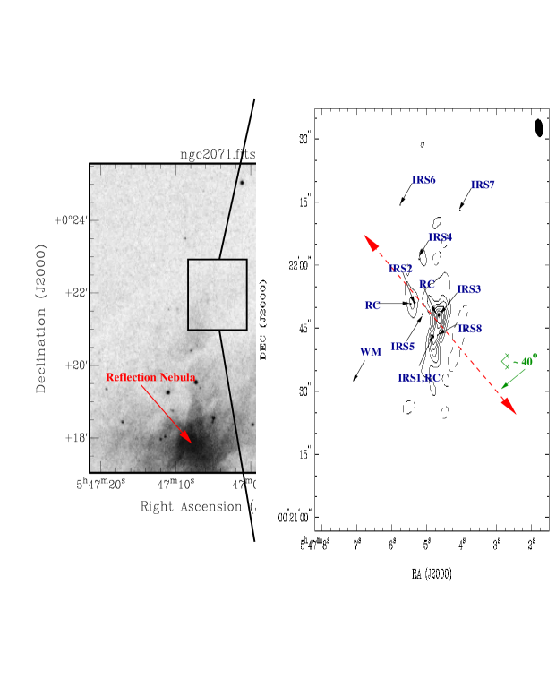
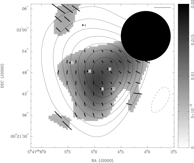
NGC2071 is a well-known optical reflection nebula located in the dark cloud Lynds 1630, which is part of the Orion complex. NGC2071IR, located 4^′ north from the reflection nebula, is a well studied region with a distance of 390 pc (Anthony-Twarog, 1982) and a size $\sim$ 30^′′. Figure 1 shows a qualitative picture of the NGC2071IR region where all the main sources are identified. The NGC2071IR region is shown as a zoom in from a bigger region which includes the NGC2071 optical reflection nebula. The NGC2071IR region has been resolved into eight distinct near-infrared sources (Walther et al., 1993) having a total luminosity of 520 $L_{\sun}$ (Butner et al., 1990). Two of them (IRS 1 and IRS 3) are associated with 5 GHz radio continuum emission from several point sources (Snell & Bally, 1986); several of these radio continuum sources may be extragalactic background objects. IRS 1 dominates the emission at near-infrared wavelengths, while IRS 3 dominates at longer wavelengths (Snell & Bally, 1986). H₂O maser emission has been detected toward NGC2071IR (Schwartz & Buhl, 1975; Pankonin et al., 1977; Campbell, 1978), particularly at IRS 1 and IRS 2, which seems to indicate the presence of substantial columns of dust-laden, warm (300-1000 K), dense gas ($10^{8}-10^{10}$ cm^-3). A 1720 MHz OH maser, located between IRS 1 and IRS 2, coincides with an H₂O maser.

A powerful molecular outflow was found in NGC2071IR (Bally, 1982); the outflow has been mapped in CO (Snell et al., 1984; Moriarty-Schieven et al., 1989), in CS (Zhou et al., 1991), and SO, SiO, and HCO⁺ (Chernin & Masson, 1992, 1993; Garay et al., 2000; Girart et al., 1999b). The origin of this outflow is attributed to IRS 1; the best evidence for this comes from H₂ observations of Aspin et al. (1992). We show the outflow direction in Figure 1. However, observations from Garden et al. (1990) show elongated molecular emission associated with IRS 3, which is only $\sim 10^{\prime\prime}$ from IRS 1. In addition, high resolution images of radio continuum emission show elongated emission which is coincident with both infrared sources (Torrelles et al., 1998; Smith & Beck, 1994; Snell & Bally, 1986). Polarimetry observations have also been made of NGC2071IR. Walther et al. (1993) made high resolution $K$ band imaging polarimetry over the whole cluster. IRS 1 and IRS 3 are highly polarized ($>30\%$ for IRS1 and $\sim 20\%$ for IRS 3), while IRS 2, IRS 4 and IRS 6 show low polarization. Matthews et al. (2002) measured continuum linear polarization toward NGC2071IR at 850 $\mu$m using the James Clerk Maxwell Telescope (JCMT). They found a polarization pattern which is ordered and qualitatively similar to other star forming regions, such as OMC-1 (Schleuning, 1998). However, they interpreted their polarization pattern differently from Schleuning (1998). The Matthews et al. (2002) polarization maps do not show the pinch seen in OMC-1; they suggested that the magnetic field morphology is inconsistent with a dynamically significant magnetic field threading the NGC2071IR core with a hourglass shape. They also concluded that the emission is dominated by dust, discarding contamination from the CO $J=3\rightarrow 2$ line from the powerful bipolar outflow that originates out of the core. Applying the Chandrasekhar-Fermi method (Chandrasekhar & Fermi, 1953), they estimated a magnetic field strength of 56 $\mu$G.

3 Observation Procedure

We observed NGC2071IR between October 2002 and May 2004, mapping the continuum emission at 1.3 mm and the CO $J=2\rightarrow 1$ molecular line (at 230 GHz). Four tracks were obtained with the BIMA array in C configuration. We set the digital correlator in mode 8 to observe both the continuum and the CO $J=2\rightarrow 1$ line simultaneously. The 750 MHz lower side band was combined with 700 MHz from the upper side band to map the continuum emission, leaving a 50 MHz window for the CO line observation (at a resolution of 1.02 km s^-1). Each BIMA telescope has a single receiver, and thus the two polarizations were observed sequentially. A quarter wave plate to select either right (R) or left (L) circular polarization was alternately switched into the signal path ahead of the receiver. Switching between polarizations was sufficiently rapid (every 11.5 seconds) to give essentially identical uv-coverage. Cross-correlating the R and L circularly polarized signals from the sky gave RR, LL, LR, and RL for each interferometer baseline, from which maps in the four Stokes parameters were produced. The source 0530+135 was used as phase calibrator for NGC2071IR. The instrumental polarization was calibrated by observing 3C279, and the “leakages” solutions were calculated from this observation. We used the same calibration procedure described by Lai (1999).

The Stokes images I, U, Q and V were obtained by Fourier transforming the visibility data using natural weighting. The MIRIAD (R. J. Sault, N. E. B. Killeen, 1998) package was used for data reduction. Both sources are close to the equator; therefore, we expect strong sidelobes in the beam pattern. We followed Chernin & Welch (1995), who observed NGC2071IR with the BIMA array, and imaged only out to 20^′′ radius, due to the strong sidelobes.

4 Observational Results

4.1 1.3 mm Continuum

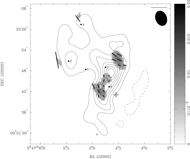
Figure 2 shows our 1.3 mm continuum intensity and polarization maps; the synthesized beam size is $4.4^{\prime\prime}\times 3.2^{\prime\prime}$ with a beam P.A. of 20.9^∘. The contours represent Stokes I with a peak emission of 0.3 Jy beam^-1. The total flux integrated over a $20^{\prime\prime}\times 30^{\prime\prime}$ box is $S_{\nu,int}=1.87$ Jy. This box defines our core in this region. The gray scale in Figure 2 corresponds to polarized flux ($\sqrt{Q^{2}+U^{2}}$) which by definition has the same units as the Stokes I emission, in this case the units are Jy beam^-1. The line segments show the P.A. and fractional polarization (which corresponds to the length of the line segments). The polarization results shown are $3\sigma$ or better, which means that all results below the $3\sigma$ threshold are cutoff from the map.

The Stokes I map resolves two components that are associated with some of the infrared sources reported by Walther et al. (1993). The first clump is located in the central part of the map corresponding to an elongated and flattened structure from north to south covering $\sim 30^{\prime\prime}$ in declination; this structure breaks up into smaller clumps with higher angular resolution. This clump seems to be associated with IRS 1, IRS 3, and IRS 8. The second clump, associated with the IRS 2 source, is located to the east of the first clump and is less significant. The rest of the infrared sources do not show significant continuum emission at 1.3 mm. Scoville et al. (1986) observed the same region with the OVRO array in 2.7 mm continuum obtaining a peak flux of 0.17 Jy. Their map shows a core of circular morphology which does not show the same elongated morphology that our observations do (see Figure 2), but this may be explained in terms of their lower resolution ($7^{\prime\prime}$) and sensitivity.

Most of the polarized emission is associated with the central and strongest clump in three distinctive regions. The northern region shows a mean P.A. of $63.4^{\circ}\pm 7.8^{\circ}$, which is polarization orthogonal to the major axis of the core. The southern region shows a mean P.A. of $21.7^{\circ}\pm 7.2^{\circ}$, while the central part shows a mean P.A. of $-15.6^{\circ}\pm 9.0^{\circ}$. Clearly, the direction of the polarization changes significantly over the elongated clump. The continuum peak presents no polarization at all (even at the $2\sigma$ level). This strong depolarization could be produced by the dust in the south producing polarization along the major axis and the dust in the north producing polarization along the minor axis of the core, which contributes roughly equally near the continuum peak position, resulting in essentially no net polarized flux. Table 1 shows P.A. and fractional polarization for NGC2071IR.

4.2 CO $J=2\rightarrow 1$

4.2.1 Description

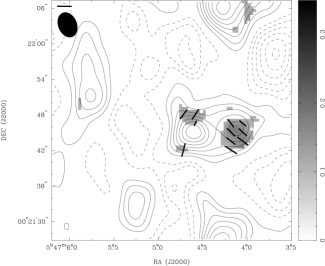
Figure 3 shows two panels with CO $J=2\rightarrow 1$ maps averaged in velocity. We used the velocity intervals: v${}_{lsr}=-7.8$ to -3.7 km s^-1 and v${}_{lsr}=+10.0$ to +23.0 km s^-1. Over v_lsr=-3.7 to +10.0 km s^-1 the polarized line flux is extremely weak. These spectral-line maps are heavily affected by missing zero and short-spacing visibility data. Nevertheless, they give at least qualitative information. The NGC2071IR molecular outflow can be seen in the blue-shifted and red-shifted maps; the emission in these maps is consistent with previous observations (Moriarty-Schieven et al., 1989; Scoville et al., 1986). The higher resolution in our maps allows us to see more detailed structure in the outflow, particularly the elongated structure in the blue-shifted lobe which is not resolved by Moriarty-Schieven et al. (1989). Also, the detection of polarized line emission provide direct evidence for the presence of a magnetic field in the outflow.

4.2.2 Polarized emission from the red-lobe

The red-shifted lobe shows predominantly one region of polarized emission, located between $\alpha=5^{h}47^{m}4.8^{s}$ to $5^{h}47^{m}3.8^{s}$, and $\delta=00^{\circ}21^{\prime}40^{\prime\prime}$ to $00^{\circ}21^{\prime}52^{\prime\prime}$. The polarized emission shows two distinctive orientations. The eastern-most region has a mean P.A. of -31.5${}^{\circ}\pm 8.7^{\circ}$ and a mean fractional polarization of 0.04$\pm 0.01$; the western region has a mean P.A. of 48.5${}^{\circ}\pm 7.9^{\circ}$ and a mean fractional polarization of 0.05$\pm 0.01$. This is a difference in P.A. of $\Delta\phi\approx 80^{\circ}$ and is consistent with orthogonal polarizations.

4.2.3 Polarized emission from the blue-lobe

The blue-shifted emission has three distinct regions of polarized emission, which are located in the north-south direction at the same right ascension ($\alpha\approx 5^{h}47^{m}5.5^{s}$). The first region is centered at $\delta=00^{\circ}21^{\prime}58^{\prime\prime}$ with mean P.A. of -50.2${}^{\circ}\pm 9.2^{\circ}$ and mean fractional polarization $0.04\pm 0.01$. The second region is centered at $\delta=00^{\circ}21^{\prime}53^{\prime\prime}$ with a mean P.A. of $53.6^{\circ}\pm 8.9^{\circ}$ and mean fractional polarization of $0.03\pm 0.01$. The third region is centered at $\delta=00^{\circ}21^{\prime}45^{\prime\prime}$ with a mean P.A. of $9.8^{\circ}\pm 8.1^{\circ}$ and fractional polarization of $0.07\pm 0.01$. The first two regions have a difference in P.A. of $\Delta\phi\sim 100^{\circ}$, again consistent with orthogonal polarization.

4.2.4 Polarized emission comparison

The P.A. for the polarized emission in both lobes have similar values. These values are orthogonal to each other and in agreement with the prediction. However, this creates an ambiguity in the interpretation of the polarization. The outflow in NGC2071IR has P.A. $\sim$ 40^∘ to 50^∘ (Moriarty-Schieven et al., 1989; Girart et al., 1999b), which is also schematically shown by Matthews et al. (2002) in their maps. Our CO polarized emission presents P.A. which are either parallel or perpendicular to the outflow direction in the plane of the sky. From this result, the projection of the magnetic field in the plane of the sky could be either parallel or perpendicular to the outflow direction. Current models for outflow suggest collimation by magnetic fields. Therefore, we believe that the most plausible interpretation is a magnetic field, which is along the outflow.

5 Discussion

We centered our observation at the same coordinates used by Matthews et al. (2002), who observed at 850 $\mu$m in the continuum using the JCMT. Their polarization map shows a uniform pattern over the core which seems to be aligned with the outflow direction (as indicated in their maps). Our continuum polarization results seem to agree reasonably well with the single dish data (Matthews et al., 2002), except for our central region, where our results appear to be orthogonal to theirs. The strength of the polarized emission is also in agreement; their mean percentage polarization at the core is about 5% while our mean percentage polarization is about 6% (see Table 1).

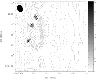
Under most conditions it is assumed that dust grains will be aligned in the presence of a magnetic field. Using this premise Matthews et al. (2002) inferred a magnetic field morphology for NGC2071IR which, they concluded, does not show the expected hourglass shape predicted by theory for a magnetically supported cloud. This conclusion seems to be in agreement with the Stokes I emission present in their maps, which does not show flattening. In order to fully compare with Matthews et al. (2002) we convolved our map with a Gaussian beam of $\sim$ 14^′′ at FWHM; the convolved map is shown in Figure 4. The lower resolution Stokes I image has all traces of flattening erased, agreeing in morphology with the contour map shown by Matthews et al. (2002). In the same way, the polarization map shows a fairly uniform profile over the core with a mean P.A. of 43.6${}^{\circ}\pm$ 4.1^∘, while the JCMT data has, over the same box, a mean P.A. of 36.9${}^{\circ}\pm$ 3.5^∘ (taken from Table 1 in Matthews et al. (2002)). We see that the sudden change in polarization P.A. in the central region of the core (shown in Figure 2) is completely lost in the lower resolution map.

Unlike the lower resolution data, our higher resolution BIMA map shows an elongated core and (if the polarization is interpreted as being due to magnetic field alignment of grains), a magnetic field that is parallel to the major axis of the core in the north, approximately orthogonal at the center, and about $45^{\circ}$ to the major axis in the south of the core. This projected field morphology would require an abrupt $90^{\circ}$ twist of the field from the north to the center. The field would then be along the minor axis at the center of the core, in agreement with a strong magnetic field model with contraction along field lines. However, at both the northern and southern edges of the core, and over the more extended region mapped with SCUBA, the field would be twisted up to $\sim 90^{\circ}$.

An alternative explanation for this polarization pattern is that grains are mechanically aligned by the powerful molecular outflow directed along the magnetic field at a P.A. $\sim 40^{\circ}$. Rao et al. (1998) observed dust polarized emission from Orion KL using the BIMA telescope at 1.3 mm. They noticed an abrupt change of 90^∘ in P.A. from one point to another in their polarization data (similar to our case), which they found difficult to explain in terms of a twisting magnetic field. They concluded that this was evidence for mechanical alignment by the powerful outflow of Orion KL. In our case, the relative alignment of the polarization pattern in Figure 2 with the outflow direction suggests mechanical alignment over most of the core (and over the more extended region mapped by SCUBA), while at the center magnetic alignment would yield a magnetic field direction consistent with the orientation of the outflows powered by IRS 1 and IRS 3. The different efficiencies of the alignment mechanism may be explained by an outflow which is not dynamically significant at the center of the core (between ISR 1 and IRS 3). This scheme seems to be consistant with the radiative torques model at similar densities (Cho & Lazarian, 2005).

We follow the formulation described by Mooney et al. (1995); Mezger et al. (1990) to calculate the column density and mass. Both quantities are give by the following equations,

$$N_{\rm{H}}/{\textnormal{cm}}^{-2}=1.93\times 10^{15}\frac{(S_{\nu,int}/\rm{Jy})\lambda^{4}_{\mu\rm{m}}}{(\theta_{s}/\rm{arcsec})^{2}(Z/Z_{\sun})bT}\frac{e^{x}-1}{x}$$ (1)

$$M_{\rm{H}}/\textnormal{M}_{\sun}=4.1\times 10^{-10}\frac{(S_{\nu,int}/\rm{Jy})\lambda^{4}_{\mu\rm{m}}D^{2}_{\rm{kpc}}}{(Z/Z_{\sun})bT}\frac{e^{x}-1}{x},$$ (2)

where $S_{\nu,int}$ is the total flux from the source, $\theta_{s}=\sqrt{\theta_{s,min}\times\theta_{s,max}}$ is the angular source size, $Z/Z_{\sun}=1$ is relative metallicity, T is the dust temperature, $b=3.4$ reproduces cross sections estimates for dust around deeply embedded IR sources (Mezger et al., 1990), $x=\frac{1.44\times 10^{4}}{\lambda_{\mu\rm{m}}T}$ is the $\frac{hc}{\lambda kT}$ factor for the Planck function, and $D_{\rm{kpc}}$ is the distance to the source in kpc. Using the obtained total flux ($S_{\nu,int}=1.87$ Jy) we calculated $N_{\rm{H}}=1.5\times 10^{23}\textnormal{cm}^{-2}$ and $M_{\rm{H}}=2.8$ $\textnormal{M}_{\sun}$. Using a $30^{\prime\prime}$ angular distance over the source, which is equivalent to $1.75\times 10^{17}\textnormal{cm}$ at a distance of 390 pc, we obtained a volume density of $n_{\rm{H}}=1.25\times 10^{6}\textnormal{cm}^{-3}$. Interstellar dust has been argued to radiate polarized emission only at low $A_{\rm{v}}$ (Goodman et al., 1995; Lazarian et al., 1997). However, using the relation between $A_{\rm{v}}$ and $N_{\rm{H}}$ given by Bohlin et al. (1978)

$$\left<N(\rm{H})/A_{\rm{v}}\right>=5.8\times 10^{21}\textnormal{cm}^{-2}\textnormal{mag}^{-1},$$ (3)

we find $A_{\rm{v}}=26$ mag, which is greater than the upper limit, $1<A_{\rm{v}}<10$ mag, proposed by Lazarian et al. (1997), which suggests that dust grains will align at higher densities than previously thought.

Houde et al. (2001) observed NGC2071IR and concluded that the magnetic field is aligned with the outflow by the comparison of widths of spectral lines of neutral and ionized species. This picture agrees with the one we discuss here. However, they did not provide direct (polarization) evidence of a magnetic field in the NGC2071IR outflow. Figure 3 shows CO $J=2\rightarrow 1$ polarized emission maps from the outflow. Line polarization is predicted in the presence of a magnetic field (Goldreich & Kylafis, 1981); therefore, this is direct evidence for a magnetic field in the outflow of NGC2071IR. The CO polarization has orthogonal position angles at different locations in both the red and blue line wings. Unfortunately, interpretation is ambiguous, for there is a $90^{\circ}$ ambiguity between the predicted polarization P.A. and the magnetic field, and the direction of line polarization can flip by $90^{\circ}$ within a region (Goldreich & Kylafis, 1981). The resolution of the ambiguity, in the general case, requires a more detailed study of the region (e.g., Cortes et al. (2005)). However, in the case of NGC2071IR outflow the coincidence between one of the polarization orientations and the outflow P.A. suggests that right interpretation is indeed, a magnetic field along the outflow. Additionally, it is also known that CO $J=2\rightarrow 1$ polarized emission will generally trace the magnetic field at a lower density from polarized dust emission, which raises the question of how the fields in the core and outflow are connected.

In summary, we suggest that the magnetic field morphology in NGC2071IR is best described as a magnetic field aligned with the bipolar outflow which would be perpendicular to the major axis of the core in Figure 2. This is consistent with a flattening of the core along magnetic field lines and allows a connection between the field in the outflow and in the core. Mechanical alignment for grains at the northern-west and southern-east edges of the map (relative to the peak in Figure 2), which will produce polarization parallel to the magnetic field (Lazarian, 1994, 1997), would explain the observed polarization morphology. However, this may require an outflow generated by both sources (IRS 1 and IRS 3), which may be possible. Also, it is important to consider that the outflow and the polarized dust emission might have different orientations with respect to the line of sight, even if their projections on the plane of the sky agree in orientation. Near the center of the core the direction of dust polarized emission cannot be explained by mechanical alignment; a possible explanation would be magnetic alignment winning over a dynamically weak outflow in that part of the core, which is consistent with a magnetic field parallel to the outflow at center of the core.

6 Summary and conclusions

We observed NGC2071IR and successfully detected CO $J=2\rightarrow 1$ line and 1.3 mm dust continuum polarized emission with a resolution of 4^′′.

We found direct evidence for a magnetic field in the outflow of NGC2071IR through CO $J=2\rightarrow 1$ polarized line emission. Also, from polarized dust emission, we suggest a magnetic field in the core along its minor axis and parallel to the outflow direction, which is consistent with the observed flattening of the core. Over most of the region the polarization is parallel to the outflow suggesting mechanical grain alignment. This interpretation provides a consistent picture for the field morphology.

We also estimated a visual extinction $A_{\rm{v}}=26$ mag relative to a column density of $N_{\rm{H}}=1.5\times 10^{23}$ cm^-2. This result suggests that the dust will polarized efficiently at greater densities than previously thought.

This research was partially funded by NSF grants AST 02-05810 and 02-28953. The BIMA array was operated with support from the National Science Foundation under grants AST-02-28963 to UC Berkeley, AST-02-28953 to U. Illinois, and AST-02-28974 to U. Maryland. BCM acknowledges funding a postdoctoral fellowship from the Natural Sciences and Engineering Research Council of Canada.

Table 1: Fractional polarization and position angle for dust polarization observations from NGC2071IR. Data were interpolated at a tolerance of 1^′′ that corresponds to approximate 1.9 $\times$ 10^-3 pc using a distance to NGC2071 of 390 pc.

Offsets in arcsec	$P_{Dust}$	$\phi_{Dust}$
(0,-6.0)	0.05$\pm$0.01	22.9$\pm$7.4
(2.0,-4.0)	0.1$\pm$0.03	16.6$\pm$8.4
(0,-4.0)	0.05$\pm$0.01	16.6$\pm$7.6
(-4.0,-6.0)	0.23$\pm$0.09	-80.3$\pm$9.2
(-2.0,-2.0)	0.03 $\pm$0.01	-17$\pm$8.9
(-3.0,-2.0)	0.03$\pm$0.01	-16.5$\pm$8.8
(-6.0,2.0)	0.06$\pm$0.02	65$\pm$9
(-4.0,4.0)	0.07$\pm$0.02	60.7$\pm$7.4
(-6.0,4.0)	0.07$\pm$0.02	66.1$\pm$7.3
(-4.0,6.0)	0.09$\pm$0.02	57.6$\pm$7.6
(5.0,18.0)	0.3 $\pm$0.1	-4.6$\pm$9.3
(3.0,18.0)	0.2$\pm$0.08	-4.2$\pm$9.2

Figure 1: The Figure shows a schematic map of the NGC2071IR region. The contours are a qualitative representation of the main core mapped. The IRS sources are shown according to the numbering given by Walther et al. (1993). Some of the IRS sources are out of the main area mapped by Figure 2. The RC sources are the radio continuum and possible background sources reported by Snell & Bally (1986). The WM source represent the H₂O maser reported by Schwartz & Buhl (1975). The NGC2071 nebula is also shown. The bipolar outflow is shown by the arrow with an overall P.A. of 40^∘.

Figure 2: Polarization map of NGC2071 at 1.3 mm. The contours represent the Stokes I emission at -0.03, 0.03, 0.07, 0.1, 0.14, 0.17, 0.21, and 0.24 Jy beam^-1. The pixel gray scale shows $3\sigma$ polarized intensity ($\sqrt{Q^{2}+U^{2}}$) for the dust continuum emission also in Jy beam^-1. The line segments are the polarization map, the length represents fractional polarization. The $\bullet$ symbols represent the IRS sources. The rms in the Stokes I map is $\sigma=0.006$ Jy beam^-1. The scale is set by 0.3 in fractional polarization shown by the bar at the upper right corner of the map.

Figure 3: The two maps represent velocity averaged CO J=$2\rightarrow 1$ polarized emission from NGC2071IR. The panel shows the red-shifted emission (left panel) and blue-shifted emission (right panel). The red-shifted emission was averaged over v${}_{lsr}=10.0$ to 23.0 km s^-1 in velocity. The contour map represents Stokes I emission at levels: -3.0, -2.4, -1.8, -1.0, -0.6, 0.6, 1.0, 1.8, 2.4, 3.0, 3.6, and 4.2 Jy beam^-1 with a maximum of 4.8 Jy beam^-1 and noise level $\sigma=0.28$ Jy beam^-1. The blue-shifted emission (right panel) was averaged over v${}_{lsr}=-7.8$ to -3.7 km s^-1 in velocity. The contour map represents Stokes I emission at levels: -4.1, -3.3, -2.4, -1.6, -0.8, 0.8, 1.6, 2.4, 3.3, 4.1, 4.9, and 5.7 Jy beam^-1 with a maximum of 6.5 Jy beam^-1 and a noise level of $\sigma=$ 0.3 Jy beam^-1. The gray scale represents $3\sigma$ polarized emission, which is also in Jy beam^-1. The length of the line segments are a representation of the fractional polarization with scale of 0.086 show by the bar at the upper left corner. The beam size is $4.4^{\prime\prime}\times 3.2^{\prime\prime}$ in both maps.

Figure 4: Convolution of Figure 2 with a gaussian beam of 14^′′ FWHM. The contours represent the Stokes I emission at -0.13, 0.13, 0.26, 0.39, 0.52, 0.65, 0.78, and 0.92 Jy beam^-1. The pixel gray scale show $3\sigma$ polarized intensity ($\sqrt{Q^{2}+U^{2}}$) measured in Jy beam^-1, for the dust continuum emission. The black line segments are the polarized dust emission map. The fractional polarization is represented by the length of the line and the P.A. by the orientation of the line segment. The scale for the line segments is given by the bar at the upper right corner which represents 0.1 in fractional polarization.

References

- Anthony-Twarog (1982) Anthony-Twarog, B. J. 1982, AJ, 87, 1213
- Aspin et al. (1992) Aspin, C., Sandell, G., & Walther, D. M. 1992, MNRAS, 258, 684
- Bachiller (1996) Bachiller, R. 1996, ARA&A, 34, 111
- Bally (1982) Bally, J. 1982, ApJ, 261, 558
- Bohlin et al. (1978) Bohlin, R. C., Savage, B. D., & Drake, J. F. 1978, ApJ, 224, 132
- Butner et al. (1990) Butner, H. M., Evans, N. J., Harvey, P. M., Mundy, L. G., Natta, A., & Randich, M. S. 1990, ApJ, 364, 164
- Campbell (1978) Campbell, P. D. 1978, PASP, 90, 262
- Chandrasekhar & Fermi (1953) Chandrasekhar, S., & Fermi, E. 1953, ApJ, 118, 113
- Chernin & Masson (1993) Chernin, L., & Masson, C. 1993, ApJ, 403, L21
- Chernin & Masson (1992) Chernin, L. M., & Masson, C. R. 1992, ApJ, 396, L35
- Chernin & Welch (1995) Chernin, L. M., & Welch, W. J. 1995, ApJ, 440, L21
- Cho & Lazarian (2005) Cho, J., & Lazarian, A. 2005, ApJ, 631, 361
- Cortes et al. (2005) Cortes, P. C., Crutcher, R. M., & Watson, W. D. 2005, ApJ, 628, 780
- Garay et al. (2000) Garay, G., Mardones, D., & Rodríguez, L. F. 2000, ApJ, 545, 861
- Garden et al. (1990) Garden, R. P., Russell, A. P. G., & Burton, M. G. 1990, ApJ, 354, 232
- Girart et al. (1999a) Girart, J. M., Crutcher, R. M., & Rao, R. 1999a, ApJ, 525, L109
- Girart et al. (1999b) Girart, J. M., Ho, P. T. P., Rudolph, A. L., Estalella, R., Wilner, D. J., & Chernin, L. M. 1999b, ApJ, 522, 921
- Goldreich & Kylafis (1981) Goldreich, P., & Kylafis, N. D. 1981, ApJ, 243, L75
- Goldreich & Kylafis (1982) —. 1982, ApJ, 253, 606
- Goodman et al. (1995) Goodman, A. A., Jones, T. J., Lada, E. A., & Myers, P. C. 1995, ApJ, 448, 748
- Houde et al. (2001) Houde, M., Phillips, T. G., Bastien, P., Peng, R., & Yoshida, H. 2001, ApJ, 547, 311
- Lai et al. (2002) Lai, S., Crutcher, R. M., Girart, J. M., & Rao, R. 2002, ApJ, 566, 925
- Lai et al. (2003) Lai, S., Girart, J. M., & Crutcher, R. M. 2003, ApJ, 598, 392
- Lai (1999) Lai, S. P. 1999, PhD thesis, University of Illinois at Urbana - Champaign, Urbana, IL 61801, not Available at the Astronomy library at the Astronomy building
- Lazarian (1994) Lazarian, A. 1994, MNRAS, 268, 713
- Lazarian (1997) —. 1997, ApJ, 483, 296
- Lazarian (2003) —. 2003, Journal of Quantitative Spectroscopy and Radiative Transfer, 79, 881
- Lazarian et al. (1997) Lazarian, A., Goodman, A. A., & Myers, P. C. 1997, ApJ, 490, 273
- Matthews et al. (2002) Matthews, B. C., Fiege, J. D., & Moriarty-Schieven, G. 2002, ApJ, 569, 304
- Mezger et al. (1990) Mezger, P. G., Zylka, R., & Wink, J. E. 1990, A&A, 228, 95
- Mooney et al. (1995) Mooney, T., Sievers, A., Mezger, P. G., Solomon, P. M., Kreysa, E., Haslam, C. G. T., & Lemke, R. 1995, A&A, 299, 869
- Moriarty-Schieven et al. (1989) Moriarty-Schieven, G. H., Hughes, V. A., & Snell, R. L. 1989, ApJ, 347, 358
- Pankonin et al. (1977) Pankonin, V., Winnberg, A., & Booth, R. S. 1977, A&A, 58, L25+
- R. J. Sault, N. E. B. Killeen (1998) R. J. Sault, N. E. B. Killeen. 1998, Miriad users guide, BIMA
- Rao et al. (1998) Rao, R., Crutcher, R. M., Plambeck, R. L., & Wright, M. C. H. 1998, ApJ, 502, L75+
- Schleuning (1998) Schleuning, D. A. 1998, ApJ, 493, 811
- Schwartz & Buhl (1975) Schwartz, P. R., & Buhl, D. 1975, ApJ, 201, L27+
- Scoville et al. (1986) Scoville, N. Z., Sargent, A. I., Sanders, D. B., Claussen, M. J., Masson, C. R., Lo, K. Y., & Phillips, T. G. 1986, ApJ, 303, 416
- Smith & Beck (1994) Smith, H. A., & Beck, S. C. 1994, ApJ, 420, 643
- Snell & Bally (1986) Snell, R. L., & Bally, J. 1986, ApJ, 303, 683
- Snell et al. (1984) Snell, R. L., Scoville, N. Z., Sanders, D. B., & Erickson, N. R. 1984, ApJ, 284, 176
- Torrelles et al. (1998) Torrelles, J. M., Gómez, J. F., Rodríguez, L. F., Curiel, S., Anglada, G., & Ho, P. T. P. 1998, ApJ, 505, 756
- Walther et al. (1993) Walther, D. M., Robson, E. I., Aspin, C., & Dent, W. R. F. 1993, ApJ, 418, 310
- Zhou et al. (1991) Zhou, S., Evans, N. J., Guesten, R., Mundy, L. G., & Kutner, M. L. 1991, ApJ, 372, 518