CMB anisotropies seen by an off-center observer in a spherically symmetric inhomogeneous universe

Abstract

The current authors have previously shown that inhomogeneous, but spherically symmetric universe models containing only matter can yield a very good fit to the SNIa data and the position of the first CMB peak. In this work we examine how far away from the center of inhomogeneity the observer can be located in these models and still fit the data well. Furthermore, we investigate whether such an off-center location can explain the observed alignment of the lowest multipoles of the CMB map. We find that the observer has to be located within a radius of $\sim 15\,\mathrm{Mpc}$ from the center for the induced dipole to be less than that observed by the COBE satellite. But for such small displacements from the center, the induced quadru- and octopoles turn out to be insufficiently large to explain the alignment.

I Introduction

In a recent work Alnes et al. (2005), we studied spherically symmetric inhomogeneous universe models – the so-called Lemaître-Tolman-Bondi (LTB) models. We found that for a certain class of inhomogeneities, such models could easily explain various cosmological observations without introducing dark energy, most notably the luminosity distance-redshift relation of type IA supernovae and the position of the first peak in the CMB spectrum. The inhomogeneities required are of the form of a spherically symmetric underdense bubble in an otherwise flat and homogeneous Einstein-de Sitter universe, with the observer located at the center of the bubble.

Unless the observer is positioned exactly at the center of the bubble, the distribution of matter, as seen by the observer, will be anisotropic. This will affect the observed microwave background and constrain the possible location of the observer, since the CMB dipole must be in agreement with observations Bennett et al. (1996). Note that in a homogeneous universe model, this dipole is attributed to the peculiar velocity of the observer. However, as discussed in Humphreys et al. (1997), in an LTB model there will be an additional contribution to the dipole from the anisotropy of space-time. Thus, the dipole seen by an off-center observer will be due to a combination of kinematic effects and the off-center location.

The anisotropy will also induce higher multipoles in the CMB spectrum. Moffat Moffat (2005) proposes this mechanism as a possible explanation for the observed alignment of the CMB quadru- and octopole de Oliveira-Costa et al. (2004); Copi et al. (2004); Schwarz et al. (2004); Ralston and Jain (2004); Land and Magueijo (2005), since the direction from the observer towards the center of the bubble singles out a “special” axis.

In this work we will investigate these induced anisotropies in the CMB to establish how far from the center the observer can be located, and whether they can offer an explanation to the alignment of the lowest multipoles. We find that the observer has to be located within a sphere extending approximately $15\,\mathrm{Mpc}$ about the origin, in order for the induced dipole to remain within the observed range. However, within this small volume the induced quadru- and octopole turn out to be insufficiently large to explain the alignment.

The paper is organized as follows: In Sect. II, we deduce the differential equations governing the path and redshift of photons. We then proceed to work out expressions for the induced temperature distribution and corresponding CMB multipoles in Sect. III. Next, in Sect. IV, we solve these equations numerically to find the multipoles as a function of the position of the observer. This allows us to find LTB models which agree with both the observed dipole and observations of SNIa and the position of the first CMB peak, as described in Alnes et al. (2005). We present two such models in this section. Finally, in Sect. V we discuss and summarize our work.

II The geodesic equation in the LTB space-time

The spherically symmetric LTB metric is given by Lemaître (1933); Tolman (1934); Bondi (1947)

$$ds^{2}=-dt^{2}+\frac{[R^{\prime}(r,t)]^{2}}{1+\beta(r)}dr^{2}+R^{2}(r,t)d\Omega^{2}\,,$$ (1)

where $R(r,t)$ is a position-dependent scale factor, and $\beta(r)$ is related to the curvature.

One of the great advantages of working in this space-time is that the Einstein equations can be solved exactly in the matter-dominated scenario. The function $R(r,t)$ can then be written in terms of a conformal time $\eta$, defined by $\beta^{1/2}dt=Rd\eta$, as

$$R = \frac{\alpha}{2\beta}(\cosh\eta-1)$$ (2)

$$+R_{0}\left[\cosh\eta+\sqrt{\frac{\alpha+\beta R_{0}}{\beta R_{0}}}\sinh\eta\right]\,,$$

$$\sqrt{\beta}t = \frac{\alpha}{2\beta}(\sinh\eta-\eta)$$ (3)

$$+R_{0}\left[\sinh\eta+\sqrt{\frac{\alpha+\beta R_{0}}{\beta R_{0}}}\left(\cosh\eta-1\right)\right]\,,$$

where $\alpha(r)\geq 0$ is an arbitrary function, and we have assumed $\beta(r)>0$. Furthermore, we have defined $R_{0}\equiv R(r,0)$, with the initial time $t=0$ defined as the time of last scattering.

Photons follow trajectories determined by the geodesic equation,

$$\frac{d^{2}x^{\mu}}{d\lambda^{2}}+\Gamma^{\mu}_{\alpha\nu}\frac{dx^{\alpha}}{d\lambda}\frac{dx^{\nu}}{d\lambda}=0\,,$$ (4)

where $\Gamma^{\mu}_{\alpha\nu}$ is the Christoffel symbol, and $\lambda$ is a monotonically increasing (or decreasing) parameter defined along the path of the photons.

Due to axial symmetry, the photon paths must be independent of the azimuth angle $\phi$, which leaves three possible choices for free index $\mu$. First, $\mu=t$ yields

$$\frac{d^{2}t}{d\lambda^{2}}+\frac{R^{\prime}\dot{R}^{\prime}}{1+\beta}\left(\frac{dr}{d\lambda}\right)^{2}+R\dot{R}\left(\frac{d\theta}{d\lambda}\right)^{2}=0\,.$$ (5)

Next, $\mu=r$ yields

$$\frac{d^{2}r}{d\lambda^{2}} + \left(\frac{R^{\prime\prime}}{R^{\prime}}-\frac{\beta^{\prime}}{2+2\beta}\right)\left(\frac{dr}{d\lambda}\right)^{2}$$ (6)

$$+ \frac{2\dot{R}^{\prime}}{R^{\prime}}\frac{dr}{d\lambda}\frac{dt}{d\lambda}-\frac{R(1+\beta)}{R^{\prime}}\left(\frac{d\theta}{d\lambda}\right)^{2}=0\,,$$

and finally, $\mu=\theta$ yields

$$\frac{d^{2}\theta}{d\lambda^{2}}+2\frac{R^{\prime}}{R}\frac{d\theta}{d\lambda}\frac{dr}{d\lambda}+2\frac{\dot{R}}{R}\frac{d\theta}{d\lambda}\frac{dt}{d\lambda}=0\,,$$ (7)

which can be written as conservation of angular momentum $J$

$$\frac{d}{d\lambda}\left(R^{2}\frac{d\theta}{d\lambda}\right)\equiv\frac{d}{d\lambda}J=0\,.$$ (8)

In addition, the 4-velocity identity, $u^{\mu}u_{\mu}=0$ for photons, leads to the constraint

$$-\left(\frac{dt}{d\lambda}\right)^{2}+\frac{(R^{\prime})^{2}}{1+\beta}\left(\frac{dr}{d\lambda}\right)^{2}+\frac{J^{2}}{R^{2}}=0\,.$$ (9)

It is simplest to specify the initial conditions at the time $t_{0}$ when the photon arrives at the observer’s position, which is given by $r=r_{0}$ and $\theta=0$. The path of the photon is shown in Fig. 1. It hits the observer at an angle $\xi$ relative to the $z$-axis. The spatial components of the unit vector along this axis are

$$v^{i}=\frac{\sqrt{1+\beta}}{R^{\prime}}(1,0,0)\,,$$ (10)

where the three components are in the $r$, $\theta$ and $\phi$ direction, respectively.

Figure 1: A photon hitting the observer at an angle $\xi$

The spatial direction $u^{i}$ is given by the tangent to the photon path at $t_{0}$, i.e.

$$u^{i}=\left|\frac{d\lambda}{dt}\right|\left(\frac{dr}{d\lambda},\frac{d\theta}{d\lambda},\frac{d\phi}{d\lambda}\right)=-\frac{1}{u}(p,J/R^{2},0)\,,$$ (11)

where the first factor ensures normalization, $g_{ij}u^{i}u^{j}=1$, and we have introduced $u\equiv dt/d\lambda$ and $p\equiv dr/d\lambda$. Note that we have chosen to let $\lambda$ decrease with time, since we will start integrating the equations at $t=t_{0}$ and follow the photons backwards in time until recombination.

The angle $\xi$ is given by the inner product of $v^{i}$ and $u^{i}$

$$\cos\xi=g_{ij}u^{i}v^{j}=-\frac{R^{\prime}}{\sqrt{1+\beta}}\frac{p}{u}\,.$$ (12)

Since the parametrization of the photon path in terms of the affine parameter $\lambda$ is arbitrary, we can choose this such that $\lambda=0$ when $t=t_{0}$ and $u_{0}=u(\lambda=0)=-1$. Using Eqs. (9) and (12), these conditions translate into the following initial conditions

$$p_{0} = \frac{\sqrt{1+\beta}}{R^{\prime}}\cos\xi\,,$$ (13)

$$J_{0} = J=R\sin\xi\,.$$ (14)

Furthermore, we need to determine the redshift of the incoming photons as a function of the direction. The photons follow a path given by $r(\lambda)$, $t(\lambda)$ and $\theta(\lambda)$. The redshift can be represented by the change in time separation between adjacent photons. Due to the expansion of the universe, this separation changes as the photons propagate through space. The redshift is given by the relative change of the separation, i.e. $z=(\tau_{r}-\tau_{e})/\tau_{e}$, where the subscripts $r$ and $e$ refer to the receiver and emitter positions, respectively.

Consider two photons emitted by a source with a time separation of $\tau$. Let the equation describing the time coordinate along the first geodesic be $t_{1}(\lambda)=t(\lambda)$. The time along the second geodesic is then given by $t_{2}(\lambda)=t(\lambda)+\tau(\lambda)$. Both photons must satisfy the 4-velocity identity (9). For the first photon this reads as

$$\left(\frac{dt}{d\lambda}\right)^{2}=\frac{R^{\prime}(r,t)^{2}}{1+\beta}\left(\frac{dr}{d\lambda}\right)^{2}+R(r,t)^{2}\left(\frac{d\theta}{d\lambda}\right)^{2},$$ (15)

while for the second photon, the 4-velocity identity becomes

$$\begin{split}\left(\frac{d(t+\tau)}{d\lambda}\right)^{2}=&\frac{R^{\prime}(r,t+\tau)^{2}}{1+\beta}\left(\frac{dr}{d\lambda}\right)^{2}\\ &+R(r,t+\tau)^{2}\left(\frac{d\theta}{d\lambda}\right)^{2}.\end{split}$$ (16)

Expanding Eq. (16) to first order in $\tau$ and using Eq. (15), we arrive at the expression

$$\frac{dt}{d\lambda}\frac{d\tau}{d\lambda}=\tau(\lambda)\left[\frac{R^{\prime}\dot{R}^{\prime}}{1+\beta}\left(\frac{dr}{d\lambda}\right)^{2}+R\dot{R}\left(\frac{d\theta}{d\lambda}\right)^{2}\right]\,.$$ (17)

The redshift measured by the observer as a function of the period at the time of emission is defined as

$$1+z(\lambda_{e})=\frac{\tau(\lambda_{r})}{\tau(\lambda_{e})}\,.$$ (18)

We differentiate this with respect to $\lambda_{e}$, which gives us the expression

$$\frac{dz}{d\lambda_{e}}=-\frac{1}{\tau(\lambda_{e})}\frac{d\tau(\lambda_{e})}{d\lambda_{e}}\frac{\tau(\lambda_{r})}{\tau(\lambda_{e})}\,.$$ (19)

Next, using Eqs. (17) and (18), and suppressing the subscript $e$, we arrive at the equation

$$\frac{dz}{d\lambda}=-(1+z)\frac{d\lambda}{dt}\left[\frac{R^{\prime}\dot{R}^{\prime}}{1+\beta}\left(\frac{dr}{d\lambda}\right)^{2}+R\dot{R}\left(\frac{d\theta}{d\lambda}\right)^{2}\right]\,.$$ (20)

This equation determines the change in redshift measured by the observer along an infinitesimal distance $d\lambda$. To find the redshift as a function of $\lambda$ for a photon hitting the observer today, we can sum up the infinitesimal contributions along the past light cone,

$$\frac{d\ln(1+z)}{d\lambda}=-u^{-1}\left[\frac{R^{\prime}\dot{R}^{\prime}}{1+\beta}p^{2}+\frac{\dot{R}}{R^{3}}J^{2}\right]\,,$$ (21)

with the initial condition $z(\lambda=0)=z_{0}=0$.

To summarize, we must solve the five first-order differential equations for ($t,r,\theta,p$ and $z$), with the corresponding initial conditions ($t_{0},r_{0},0,p_{0}$ and $z_{0}$), under the constraints (9) and (14).

III Temperature anisotropies

We wish to examine how being situated away from the center of the LTB coordinate system affects the CMB temperature measured by the observer. Since space-time is no longer spherically symmetric around such an observer, we expect him to measure additional anisotropies in the temperature to those measured by an observer at the center. In this paper we concentrate on the additional anisotropies rising from the observer’s location, i.e. we disregard any intrinsic anisotropies in the CMB temperature at the last-scattering surface. Thus, we assume the temperature at the last-scattering surface to be isotropic. Any anisotropies measured by observers today are therefore due to the propagation of photons through an anisotropic space-time.

The temperature of the background radiation in a given direction is determined by measuring the intensity of incident photons from this direction. Assuming the radiation to be black-body radiation, the intensity will be given by a Planck spectrum with a corresponding characteristic temperature. It can be shown that the radiation field preserves its black-body nature as it propagates freely through space under the influence of a gravitational field Ellis (1971). At any later time, the spectrum will still remain a Planck spectrum, but with a different temperature.

In our specific case, the CMB temperature seen today by an off-center observer is given by

$$T(\xi)=\frac{T_{*}}{1+z(\xi)}\,,$$ (22)

where $T_{*}$ is the temperature at the last-scattering surface, and $\xi$ is the angle defined in Fig. 1. The average temperature $\widehat{T}$ measured by the observer is then

$$\widehat{T}\equiv\frac{1}{4\pi}\int\!d\Omega\,T(\xi)=\frac{T_{*}}{2}\int_{0}^{\pi}d\xi\frac{\sin{\xi}}{1+z(\xi)}\,.$$ (23)

According to measurements made by the COBE satellite Mather et al. (1999), this temperature is $\widehat{T}=2.725$. We can now use Eqs. (22) and (23) to define an average redshift to the last-scattering surface:

$$1+z_{*}\equiv\frac{T_{*}}{\widehat{T}}=2\left[\int_{0}^{\pi}\!d\xi\frac{\sin{\xi}}{1+z(\xi)}\right]^{-1}\,.$$ (24)

The relative temperature variation measured by the observer today will then be

$$\Theta(\xi)\equiv\frac{\Delta T}{\widehat{T}}=\frac{T(\xi)-\widehat{T}}{\widehat{T}}=\frac{z_{*}-z(\xi)}{1+z(\xi)}\,.$$ (25)

It is often more interesting to consider contributions at different angular scales rather than the total anisotropy itself. Such an analysis can be performed by decomposing the temperature field in spherical harmonics $Y_{lm}$:

$$\Theta(\xi)=\sum_{l,m}a_{lm}Y_{lm}\,,$$ (26)

where the amplitudes in the expansion are recovered as

$$a_{lm}=\int_{0}^{2\pi}\!\int_{0}^{\pi}\!\Theta\,Y_{lm}^{*}\sin{\xi}\,d\xi\,d\phi\,.$$ (27)

These measure the level of anisotropy at different angular scales, with larger $l$ values corresponding to smaller scales. Since the relative temperature field does not depend on the azimuth angle $\phi$, all the $a_{lm}$ will vanish, except those with $m=0$.

The observed dipole in the CMB is of the order $|a_{10}|\sim 10^{-3}$. This will put a natural constraint on how far away from the origin the observer can be located, since a farther off-center position usually means a larger dipole.

IV Numerical results

Following Alnes et al. (2005) we will consider LTB models where the inhomogeneity is an underdense bubble with a flat and homogeneous space-time outside. We will consider two specific models of this type corresponding to two different choices of the functions $\alpha(r)$ and $\beta(r)$ in Eqs. (2) and (3). We will refer to these as model I and model II. We parametrize these function in the same way as in Alnes et al. (2005), i.e. we write

$$\alpha(r) = H_{0}^{2}r^{3}\left[\alpha_{0}-\Delta\alpha\left(\frac{1}{2}-\frac{1}{2}\tanh\frac{r-r_{0}}{2\Delta r}\right)\right]$$ (28)

$$\beta(r) = H_{0}^{2}r^{2}\left[\beta_{0}-\Delta\beta\left(\frac{1}{2}-\frac{1}{2}\tanh\frac{r-r_{0}}{2\Delta r}\right)\right]$$ (29)

which corresponds to a smooth interpolation between two homogeneous regions (i.e. a spherical bubble in an otherwise homogeneous universe). The parameter $H_{0}=100\,h_{\text{out}}\mathrm{km\,s^{-1}Mpc^{-1}}$ is the Hubble constant of the outer homogeneous region today, while $\alpha_{0}$ and $\beta_{0}=1-\alpha_{0}$ are the relative densities of matter and curvature in this region. Further, $\Delta\alpha=-\Delta\beta$ determines the difference in matter density between the regions, while $r_{0}$ and $\Delta r$ specify the position and width of the transition.

In our previous work Alnes et al. (2005), we assumed that the observer was positioned at the center of the bubble, and found a model that gave a good agreement with the Hubble diagram of observed SNIa and the position of the first CMB peak. Model I is identical to this model, while model II is slightly different. The matter distribution today for these models is plotted in Fig. 2, where we have used the generalized matter density defined in Alnes et al. (2005). Various other properties of these are listed in Tab. 1. One notable difference between these two models is that the transition from the underdensity to the homogeneous region is much sharper in the second model. Note that the physical values given in the table are found assuming that the observer is placed at the center. The shift parameter $\mathcal{S}$ is defined in Alnes et al. (2005), and is simply the shift of the first peak in the CMB power spectrum relative to the concordance $\Lambda$CDM model. As we can see, both models yield a very good fit to both SNIa and the first CMB peak.

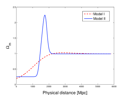
Figure 2: The matter density today as a function of physical distance for the two models considered.

Description	Symbol	Model I	Model II
Density contrast parameter	$\Delta\alpha$	0.90	0.78
Transition point [Gpc]	$d_{0}$	1.34	1.68
Transition width	$\Delta d/d_{0}$	0.40	0.03
Fit to supernovae	$\chi^{2}_{SN}$	176.2	177.8
Position of first CMB peak	$\mathcal{S}$	1.006	1.002
Age of the universe [Gyr]	$t_{0}$	12.8	12.7
Relative density at the center	$\Omega_{m,in}$	0.20	0.25
Relative density outside underdensity	$\Omega_{m,out}$	1.00	1.00
Hubble parameter at the center	$h_{in}$	0.65	0.63
Hubble parameter outside underdensity	$h_{out}$	0.51	0.51

Table 1: The parameters and features of two inhomogeneous models, with the observer placed at the center. Note that $d_{0}$ and $\Delta d$ are physical distances corresponding to $r_{0}$ and $\Delta r$

Figs. 3 and 4 show the solutions of the geodesic equations for two off-center observers in the two models, with the observers located $20\,\mathrm{Mpc}$ and $200\,\mathrm{Mpc}$ from the center. The blue lines show the photon paths in the metric ($r,\theta$) space, while the red circles are the positions of incoming photons at evenly spaced points in (cosmic) time.

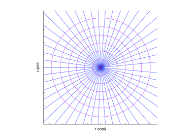
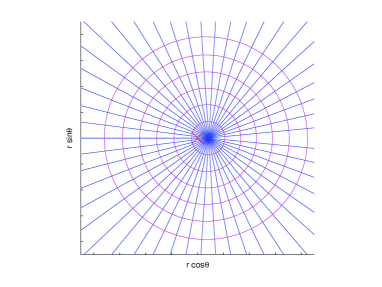
Figure 3: Model I: Photon paths converging on the observer located $20\,\mathrm{Mpc}$ (top) and $200\,\mathrm{Mpc}$ (bottom) from the center. The red cross marks the center of the underdensity, while the red circles show positions that are evenly spaced in cosmic time with a separation of $1\,\mathrm{Gyr}$

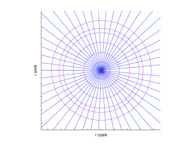
Figure 4: Model II: Photon paths converging on the observer located $20\,\mathrm{Mpc}$ (top) and $200\,\mathrm{Mpc}$ (bottom) from the center. The red cross marks the center of the underdensity, while the red circles show positions that are evenly spaced in cosmic time with a separation of $1\,\mathrm{Gyr}$

The distortion of light paths is clearly visible on the bottom plot of Fig. 4, in which the observer is placed relatively far from the center of the inhomogeneity and the density gradient is large at the transition.

In our calculations, recombination is assumed to occur at $t=0$ and today ($t_{0}$) is defined to be the time when the redshift of photons emitted at $t=0$ reaches $z_{*}\simeq 1100$. (The exact value of $z_{*}$ depends on the matter density outside the bubble, and a fitting formula is given in Doran and Lilley (2002)).

As discussed in the previous section, an off-center observer will measure a temperature anisotropy due to the non-symmetric paths traversed by CMB photons in different direction in the sky. Using Eqs. (26) and (27), we can now calculate the temperature multipoles seen by such an observer. As an example, a plot of the multipoles can be seen in Fig. 5 for an observer who is located $200\,\mathrm{Mpc}$ from the center in model I.

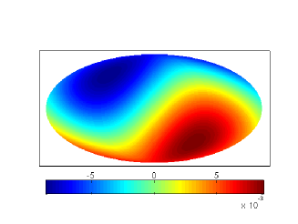
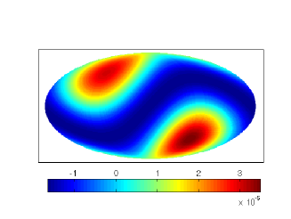
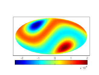
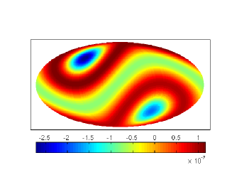
Figure 5: Temperature anisotropy in galactic coordinates seen by an observer $200\,\mathrm{Mpc}$ from the center of Model I, oriented so that the induced dipole coincides with the direction of the dipole seen by the COBE satellite Mather et al. (1999). The top plot to the left shows the temperature map, which is completely dominated by the dipole. Then follow plots with the dipole, quadrupole and octopole removed, successively

In Fig. 6, the coefficients $a_{l0}$ for the dipole ($l=1$), quadrupole ($l=2$) and octopole ($l=3$) are plotted as functions of the observer’s position in model I.

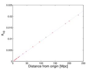
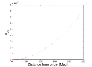
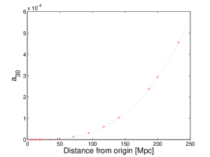
Figure 6: The $a_{l0}$ as a function of the observer’s position, in Model I. The dotted lines are linear, quadratic and cubic fits, respectively.

The most striking feature of these plots is that the quadru- and octopoles are very small compared to the dipole. If we assume that the induced dipole must be smaller than $10^{-3}$, the induced quadrupole is less than $10^{-7}$ while the induced octopole is smaller than $10^{-9}$.

In Fig. 7, the $a_{l0}$’s of model II are plotted as functions of the observer’s position.

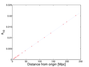
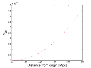
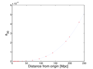
Figure 7: The $a_{l0}$ as a function of the observer’s position, in Model II. The dotted lines are linear, quadratic and cubic fits, respectively.

It is evident that the behavior is almost indistinguishable from that of Model I, except for the largest distances where the transition from underdensity to flat space is starting to show in the first model.

V Discussion

The main purpose of this paper has been to determine the maximum displacement of the observer from the origin of the underdensity, for which the induced CMB dipole remains in agreement with the results observed by COBE Bennett et al. (1996). Of course, one could in principle introduce an additional peculiar velocity towards the center of the underdensity to compensate for a too large induced dipole, but such a coincidence would be very difficult to justify. Therefore, we must require the induced $a_{10}$ to be of order $10^{-3}$ or less, which from the plots in Figs. 6 and 7 can be translated to

$$d_{obs}\lesssim 15\,\mathrm{Mpc}\,.$$ (30)

where $d$ is the physical distance. When compared to the size of the underdensity, which according to Fig. 2 is around 1 500 Mpc, this means that if we are placed at a random position inside the bubble, there is roughly a chance of $1$ to $10^{6}$ that we end up inside the region allowed by Eq. (30). This is a rather strong violation of the Copernican principle, which states that we are not situated at a special place in the universe. On the other hand, a $10^{-6}$ probability is still much better than the infinitely improbable case of the observer being exactly at the center of the underdensity. Note that the size of the underdensity is dictated by the fit to the CMB and SNIa data. We have not been able to find smaller bubbles that fit these data as well as the models considered here.

From Figs. 6 and 7 we see that the induced multipoles become larger the farther away from the origin the observer is located, as we would expect. Thus, the largest possible quadru- and octopoles with a dipole compatible with COBE measurements are those for an observer about $15\,\mathrm{Mpc}$ from the origin. However, at this relatively small distance, the values for these are of the order $10^{-7}$ for the quadrupole, and $10^{-9}$ for the octopole. It is therefore clear that the induced quadru- and octopole cannot explain the observed alignment of the low-l multipoles in the CMB, since their contributions are negligible compared to the observed anisotropies (which are of order $10^{-5}$). Furthermore, any off-center placement must necessarily result in axial symmetric contributions to the CMB spectrum. Even if such contributions were of the correct order, Rakić et al. Rakić et al. (2006) show that they are very unlikely to explain the alignment.

The smallness of the induced multipoles can be understood from a simplified Newtonian picture. Compared to the homogeneous case with a spatially constant Hubble parameter $h_{out}$, the observer at $d_{obs}$ has a “peculiar velocity” of roughly

$$\beta=\frac{v_{p}}{c}=\frac{h_{in}-h_{out}}{3000\,\mathrm{Mpc}}d_{obs}$$ (31)

with respect to the origin. In such a picture, the temperature anisotropies measured by the observer are attributed to a Doppler shift of the CMB photons due to his motion. The change in frequency can then be written as Jackson (1999)

$$\frac{\nu_{o}}{\nu_{e}}=\frac{\sqrt{1-\beta^{2}}}{1-\beta\cos{\xi}}\,,$$ (32)

where $\nu_{o}$ is the frequency measured by the observer, and $\nu_{e}$ is the frequency relative to a stationary background. The temperature shift associated with this frequency shift of the CMB photons is

$$\frac{T_{o}}{T_{e}}=\frac{\sqrt{1-\beta^{2}}}{1-\beta\cos{\xi}}\,.$$ (33)

The average background temperature measured by the observer will then be

$$\widehat{T}_{o}=\frac{1}{4\pi}\!\!\int d\,\Omega T_{o}(\xi)=\frac{T_{e}}{2}\frac{\sqrt{1-\beta^{2}}}{\beta}\ln{\left(\frac{1+\beta}{1-\beta}\right)}\,.$$ (34)

Thus, the temperature anisotropy can be written as

$$\Theta(\xi)=\frac{\Delta T(\xi)}{\widehat{T}_{o}}=\frac{2}{\ln{\left(\frac{1+\beta}{1-\beta}\right)}}\frac{\beta}{1-\beta\cos{\xi}}-1\,.$$ (35)

Using Eq. (27), the multipoles can now be calculated in terms of the velocity of the observer. We find that the leading contribution to $a_{l0}$ is $\beta^{l}$,

$$a_{l0}\sim\beta^{l}\sim d_{obs}^{l}\,.$$ (36)

Thus, using this simplified Newtonian picture, we expect the dipole to scale linearly, the quadrupole quadratically, and the octopole cubically with the observers position. In Figs. 6 and 7 we have plotted the real dependence of these multipoles on the observers position along with a best-fit $d_{obs}^{l}$ dependence. As we see, the Newtonian picture gives a very good description. The expressions for the three lowest multipoles to the lowest order in $\beta$ is

$$a_{10}= \sqrt{\frac{4\pi}{3}}\frac{h_{in}-h_{out}}{3000\,\mathrm{Mpc}}d_{obs}\,,$$ (37)

$$a_{20}= \sqrt{\frac{16\pi}{45}}\left(\frac{h_{in}-h_{out}}{3000\,\mathrm{Mpc}}\right)^{2}d_{obs}^{2}\,,$$ (38)

$$a_{30}= \sqrt{\frac{16\pi}{175}}\left(\frac{h_{in}-h_{out}}{3000\,\mathrm{Mpc}}\right)^{3}d_{obs}^{3}\,.$$ (39)

Numerically, this approximation yields $a_{10}=1.4\times 10^{-3}$, $a_{20}=5.2\times 10^{-7}$ and $a_{30}=1.2\times 10^{-9}$ for an observer at $d_{obs}=15\,\mathrm{Mpc}$ in Model I, whereas the exact values are $a_{10}=1.4\times 10^{-3}$, $a_{20}=2.3\times 10^{-7}$ and $a_{30}=1.3\times 10^{-9}$ respectively.

Eqs. (37)-(39) imply that it is impossible to obtain sufficiently large values for the quadru- and octopole as long as the dipole is within the limits set by the COBE data. Note, however, that Tomita Tomita (2000) has previously found relatively large values for the quadrupole in more simplified bubble models (where two homogeneous regions are separated by a massive comoving shell). It is unclear to us why the Newtonian approach fails for his models. We have attempted to reproduce his results by introducing very narrow transition regions in our continuous model, but the results we get for the multipoles are of the same order as those quoted above. We therefore expect Eq. (36) to be roughly correct for all models of our type.

In our analysis so far we have only considered contributions to the multipoles from the off-center placement. There will of course be additional contributions from various sources such as the intrinsic primordial temperature anisotropies, the integrated Sachs-Wolfe (ISW) effect Sachs and Wolfe (1967) and a non-vanishing peculiar velocity of the observer. We have seen that when the dipole is constrained by data, the quadru- and octopoles due to the off-center placement are considerably weaker than those observed in the CMB. A possible way to obtain stronger quadru- and dipoles is to place the observer farther away from the center, while allowing one or more of the effects mentioned above to cancel out the excessive contribution to the dipole.

However, concerning the first two effects, it is clear that neither of these can achieve such cancellation. Although there is no way of measuring directly the intrinsic dipole, it is reasonable to assume that it is of the same order as the neighboring multipoles, which are of order $10^{-5}$ Similarly, we expect the contribution to the dipole from the ISW effect to be of the same order as for the quadru- and octopole. Therefore, it is very unlikely that these effects are responsible for a chance cancellation of an excessive contribution to the dipole from the off-center placement.

A non-vanishing peculiar velocity can reduce the dipole to any desired value as long as the velocity is chosen large enough. However, multipoles due to such motion will have a hierarchical scaling similar to that which we showed in the Newtonian case. Thus, even if we manage to obtain values for the dipole and quadrupole of the correct order, the octopole would still be too weak. From this we can conclude that even when combined with other effects, the off-center placement cannot provide sufficient power to both the quadru- and octopole.

In summary, LTB models like the ones listed in Table 1 are not ruled out on the basis of these results, but they do require a violation of the Copernican principle, since the observer would have to be located at a very special place. The volume within which the observer can be located is severely constrained by the size of the dipole induced by an off-center placement of the observer. As a consequence of this, the quadru- and octopole turn out to have insufficient power to explain the observed alignment. However, the LTB models remain an exotic alternative to dark energy as an explanation of the apparent accelerated expansion of the universe.