Signals from the Noise: Image Stacking for Quasars in the FIRST Survey

Abstract

We present a technique to explore the radio sky into the nanoJansky regime by employing image stacking using the FIRST survey. We begin with a discussion of the non-intuitive relationship between the mean and median values of a non-Gaussian distribution in which measurements of the members of the distribution are dominated by noise. Following a detailed examination of the systematic effects present in the 20 cm VLA snapshot images that comprise FIRST, we demonstrate that image stacking allows us to recover the average properties of source populations with flux densities a factor of 30 or more below the rms noise level. With the calibration described herein, mean estimates of radio flux density, luminosity, radio loudness, etc. are derivable for any undetected source class having arcsecond positional accuracy.

We demonstrate the utility of this technique by exploring the radio properties of quasars found in the Sloan Digital Sky Survey. We compute the mean luminosities and radio-loudness parameters for 41,295 quasars in the SDSS DR3 catalog. There is a tight correlation between optical and radio luminosity, with the radio luminosity increasing as the 0.85 power of optical luminosity. This implies declining radio-loudness with optical luminosity: the most luminous objects ($\mbox{$M_{UV}$}=-28.5$) have on average three times lower radio-to-optical ratios than the least luminous objects ($\mbox{$M_{UV}$}=-20$). There is also a striking correlation between optical color and radio loudness: quasars that are either redder or bluer than the norm are brighter radio sources. Quasars having $g-r\sim 0.8$ magnitudes redder than the SDSS composite spectrum are found to have radio-loudness ratios that are higher by a factor of 10. We explore the longstanding question of whether a radio-loud/radio-quiet dichotomy exists in quasars, finding that optical selection effects probably dominate the distribution function of radio loudness, which has at most a modest ($\sim 20$%) inflection between the radio-loud and radio-quiet ends of the distribution. We also examine the radio properties of the subsample of quasars with broad absorption lines, finding, surprisingly, that BAL quasars have higher mean radio flux densities at all redshifts, with the greatest disparity arising in the rare low-ionization BAL subclass. We conclude with examples of other problems for which the stacking analysis developed here is likely to be of use.

1. Introduction

“Blank sky” is rarely truly blank. All astronomical imaging observations have a sensitivity threshold below which “objects” are not detectable. Assuming a reasonably linear detector response, however, it is not necessarily the case that zero photons from discrete sources have been detected at a given “blank” spot in an image. If one has reason to believe from observations in another wavelength regime that discrete emitters are present at a set of well-specified locations, it is possible to usefully constrain, or even to detect, the mean flux of that set of emitters by stacking their “blank sky” locations. The prerequisites for successfully stacking images in this way are good astrometry for both the target objects and the survey images, and sufficient sky coverage to include a large sample of the target class.

In an early application of this technique, Caillault & Helfand (1985) detected the mean X-ray flux from undetected G-stars in the Pleiades, using it to constrain the decay of stellar X-ray emission with age. As higher-resolution X-ray mirrors and detectors have become available over the past two decades, X-ray stacking has become a standard analysis technique. Applications have ranged from determining the mean X-ray luminosity of object classes in deep X-ray images — e.g., normal galaxies (Brandt et al. 2001a), Lyman Break galaxies (Brandt et al. 2001b), and radio sources (Georgakakis et al. 2003) — to determining the X-ray cluster emission from distant clusters in the Rosat All-Sky Survey (Bartelmann & White 2003).

As linear digital detectors have come to dominate optical and infrared sky surveys, the stacking technique has been widely adopted: e.g., Zibetti et al. (2005) detected intracluster light by stacking 683 Sloan Digital Sky Survey (SDSS) clusters, Lin et al. (2004) stacked 2MASS data on cluster galaxies, Hogg et al. (1997) stacked Keck IR data to get faint galaxy colors, and Minchin et al. (2003) went so far as to stack digitized films from the UK Schmidt telescope to complement a deep H I survey with the Parkes multi-beam receiver. Scaramella et al. (1993) have even stacked cosmological simulations in investigating the Sunyaev-Zeldovich effect on the cosmic microwave background.

The radio sky is relatively sparsely populated with sources. The deepest large-area sky survey, FIRST, has a surface density of only $\sim 90$ sources deg^-2 at its 20 cm flux density threshold of 1.0 mJy. Fluctuation analysis of the deepest radio images ever made suggest a source surface density of $\sim 15$ arcmin^-2 at $\sim 1~{}\mbox{$\mu$Jy}$ (Windhorst et al. 1993); given that the mean angular size of such sources is $\sim 2.4\arcsec$, even at these flux density levels only $\sim 3\%$ of the sky is covered by radio emission. Nonetheless, applications of stacking in the radio band have been limited. Recently, Serjeant at el. (2004) stacked SCUBA data to find the mean submillimeter flux of Spitzer $24~{}\mu$m-selected galaxies. It is with large-area surveys and large counterpart catalogs, however, that the stacking technique allows one to reach extremely faint flux density levels unachievable by direct observations.

The FIRST survey (Becker, White, & Helfand 1995) is ideally suited for stacking studies. It contains 811,000 sources brighter than $\sim 1~{}\mbox{mJy}$ over 9030 deg² of the northern sky and has an angular resolution of $5\arcsec$. Thus, over 99.9% of its five billion beam areas represent blank sky. Having written several dozen papers on sources detected in the survey, we turn here to analyzing the remaining 99.9% of the data. Glikman et al. (2004b) presented our initial results of applying radio image stacking to the FIRST survey. Wals et al. (2005) applied this technique to the 2dF quasar catalog (Croom et al. 2004) using FIRST images, producing an estimate of the mean flux density for undetected quasars in the range $20-40~{}\mbox{$\mu$Jy}$. In this paper, we describe the set of detailed tests we have carried out to calibrate biases in the FIRST survey’s VLA images in order to put stacking results on a quantitative basis, and we illustrate the technique with several examples. Subsequent papers will apply these results to various problems of interest.

We begin (§2) with a discussion of the median stacking procedure that we have adopted, exploring in some detail the meaning of, and distinctions between, mean and median values in data dominated by noise. We go on to provide a thorough analysis of the noise characteristics of the FIRST images, both by stacking known sub-threshold sources and by the use of artificial sources inserted into the survey data (§3). We find a non-linear correction to the flux densities derived from a stacking analysis, which most likely arises from the application of the highly nonlinear ‘CLEAN’ algorithm to these undersampled $uv$ (snapshot) data. We then apply our calibrated stacking procedure to the SDSS DR3 quasar survey from Schneider et al. (2005) (§4). In addition to deriving quasar radio properties as a function of redshift and optical color, we reexamine the issue of whether the radio-loudness distribution is bimodal. We also explore the distinction between broad absorption line (BAL) and non-BAL objects, finding the surprising result that BAL quasars have a higher mean flux density and radio loudness than non-BAL objects below 2 mJy. We conclude (§5) with a summary of the implications of our results, and preview other applications of our stacking procedure.

2. Mean Versus Median Stacking Procedures

We have explored two different methods for stacking sub-threshold FIRST images, one using the mean of each pixel in the stack and the other using the median. Both approaches have advantages and disadvantages. The mean flux density in a stacked image is mathematically simple and is easily interpretable. However, it is very sensitive to the rare outliers in the distribution. The presence of a bright source in the stack, either at the image center or in the periphery, makes itself obvious in the summed image. Moreover, noise outliers can also cause problems, as a minority of very noisy images may substantially raise the noise in the mean image. The outlier problem can be addressed by testing each image in the stack, discarding sources that are actually above the FIRST detection threshold and/or discarding images that exceed some rms noise threshold. However, the resulting mean is sensitive to the exact value of the discard threshholds and hence does not provide a very robust measurement.

The alternative is to determine the median value of the stacked images. The obvious advantage is the insensitivity of the median to outliers, since the median is well known to be robust in the presence of non-Gaussian distributions (e.g., Gott et al. 2001). Therefore all of the data can be utilized, eliminating the need to impose an arbitrary cutoff to the distribution. However, the interpretation of the median value for low signal-to-noise (S/N) data is not straightforward. For high S/N data, the median is simply the value at the midpoint of the distribution. But in the case of low S/N data, the value obtained by taking the median is shifted from the true median toward the ‘local’ mean value. The degree of the shift depends on the amplitude of the noise; as the noise increases, the recovered value approaches the ‘local’ mean, where the ‘local’ mean is the mean of the values within approximately one rms of the median. Hence the recovered median value can depend on both the intrinsic distribution of the parameter and the noise level.

Figure 1.— The effect of measurement noise on the measured median value for a skewed distribution. (a) A distribution consisting of two equal Gaussians, a wide component at $x=1$ and a narrow component at $x=0$. (b) A distribution composed of two exponentials having very different scale heights with the broad component including only a small fraction of the population. The probability has been multiplied by $x$ for a better visual display of the distribution plotted versus $\log\,x$. (c) The median for the double Gaussian distribution with noise added shows a smooth transition. When the noise is small, we recover the true median, and as the rms noise becomes comparable to the separation of the components, the value converges to the mean for the distribution. (d) The median for the double exponential distribution with noise presents a transition from the true median to the mean that pauses at the mean for the dominant (narrower) population.

Some concrete examples may help to illuminate this effect. Figure 1 shows the dependence of the measured median value (computed using numerical integration) on the noise level for two asymmetrical distributions. First consider a simple distribution consisting of two Gaussians centered at $x_{1}=0$ and $x_{2}=1$ with widths $\sigma_{1}=0.1$ and $\sigma_{2}=0.5$ (Fig. 1a). The Gaussians are normalized to have equal integral amplitudes, but because the first is much narrower, its peak is higher by a factor of $\sigma_{2}/\sigma_{1}=5$. The mean of the distribution is midway between the Gaussians at $\langle x\rangle=0.5$, but the median is dominated by the much better-localized narrow component and falls at median$(x)=0.167$. If samples are drawn from this distribution with additive Gaussian measurement noise, the peaks of both distributions get broadened. In the limit where the noise is much larger than $x_{2}-x_{1}$, the median value converges to the mean $\langle x\rangle$. The transition with increasing values of the noise rms is shown in Figure 1(c).

The general shape of the transition in Figure 1(c) is typical for simple skewed distributions (e.g., power laws, exponentials, etc.). However, more complicated distributions display a more complex dependence on the noise level. Figure 1(b) shows a distribution composed of two one-sided exponentials, $P(x)dx=\exp(-x/h)/h$, with $x>0$. The first exponential drops rapidly, with a scale height $h_{1}=1$, while the second drops much more slowly, $h_{2}=1000$. The two components are normalized so that the first contains the vast majority of the sources, with the integrated amplitude of the second component being only 0.05% of the total. When Gaussian noise is added, there are three separate regimes of behavior (Fig. 1d). When the rms noise is much smaller than either exponential scale, the true median is recovered: median$(x)=0.694$, just slightly above the median computed for component 1 only ($\ln 2=0.693$). For very large rms noise levels the measured median converges to the mean for the whole distribution ($\langle x\rangle=1.50$). But for intermediate values of the rms around unity, there is an inflection where the measured median value pauses at a value of median$(x)\sim 1$. This is explained by the fact that the dominant exponential with $h_{1}=1$ is itself a skewed distribution having a mean $\langle x\rangle_{1}=1$.

It is worth noting that the standard arithmetic mean is also of limited utility in the presence of complex multiple-component, strong-tailed distributions like that in Figure 1(b). Even for those distributions the median is generally a better match to one’s intuitive concept of the “typical” value of the distribution.

Despite these complications (about which we have found little discussion in the astronomical literature), we believe that the median is distinctly preferable to the mean for stacking our FIRST survey images. In our tests, the robust median calculation produces significantly more stable results with lower noise, while giving very similar measured values for the fluxes. We are in a limit where almost all the values in our sample are small compared with the noise, so it is straightforward to interpret our median stack measurements as representative of the mean for the population of sources with flux densities fainter than a few times the FIRST rms (i.e., a few $\times 0.145~{}\mbox{mJy}$). Throughout the paper, we refer to the median-derived approximate mean interchangeably as the “median” or “average” of the quantity of interest.

3. Calibration of the Stacking Procedure

3.1. Introduction

As an aperture synthesis interferometer, the Very Large Array samples the Fourier transform of the radio brightness distribution on the sky. To obtain a sky image requires transforming to the image plane with incomplete information. The 165-second snapshots that comprise the FIRST survey are particularly problematic in this regard: we typically obtain $\sim 30,000$ visibility points and transform them into images with $\sim 5\times 10^{5}$ resolution elements. The nonlinear algorithm ‘CLEAN’ (Högbom 1974; Clark 1980) is used to minimize artifacts such as the diffraction spikes produced by the VLA geometry and the grating rings imposed by the minimum antenna spacings employed.

One consequence of this process, discovered in the course of the NVSS (Condon et al. 1998) and FIRST surveys, is “CLEAN bias”. This incompletely understood phenomenon steals flux from the above-threshold sources and redistributes it around the field. The magnitude of the bias is dependent on the rms noise in the image (it increases as noise increases), the off-axis angle (it decreases in consort with the primary beam pattern), and the source extent (extended sources lose more flux). The FIRST and NVSS surveys took considerable pains to calibrate CLEAN bias, concluding, respectively, that it had values of 0.25 mJy/beam and 0.30 mJy/beam. (It is unsurprising that the different resolutions, integration times, and analysis procedures of the two surveys produced slightly different results).

While the sources of interest in a stacking analysis are sub-threshold and therefore, by definition, have not been CLEANed, we have taken the discovery of CLEAN bias as a cautionary tale and have examined in detail the behavior of our images subjected to the stacking process. We find that we do not recover the full flux density of either artificial sources inserted into the images or real sub-threshold sources. We describe here our calibration of this phenomenon, which we dub “snapshot bias”.

3.2. Artificial source tests

The Astronomical Image Processing System (AIPS) used to reduce VLA data includes a task UVMOD that allows the user to insert artificial sources into a $uv$ database in order to test the fidelity of the analysis. Since in this case we are interested in sources far below the detection threshold, a large number of artificial sources is required. The median rms in coadded FIRST fields is 145 $\mu$Jy; thus, to achieve an uncertainty of $\sim 10\%$ in the measured flux density of, say, 40 $\mu$Jy sources requires the addition of more than 1200 individual sources.

For our initial attempt to measure the bias, we inserted one hundred 40 $\mu$Jy sources placed in a regular square grid into each of 100 FIRST fields. This approach allowed us to minimize the number of maps we needed to make. However, this failed as a consequence of the interference of the sidelobe patterns that even these very faint sources produce. Constructive and destructive interference of sidelobes led to noise in the stacked images that varied strongly and systematically at different artificial source grid positions. We concluded that this test was not sufficient to measure the bias for random source locations.

Our ultimate artificial source test involved placing four 40 $\mu$Jy sources in each of 400 FIRST $uv$ datasets. The sources were placed at the corners of a square of side $\sim 2\arcmin$ centered on the image. We then CLEANed the 400 images, extracted $1\arcmin$ cutouts around each of the fake source locations, and stacked the cutouts to find the median flux density. Since artificial source locations were not screened in advance, they ocassionally fell on or near the location of a real radio source; the median algorithm effectively rejected the contaminated pixels in those cases (§2). Source parameters were derived by fitting an elliptical Gaussian to the stacked image as is done for source extraction in the real images. To improve the quality of the fits, regions around the diffraction spikes in the VLA dirty beam (see Fig. 4 below for an example) are masked out. The process was repeated for artificial sources with a peak flux density of 80 $\mu$Jy.

The results are presented in Table 1. The recovered median peak flux densities for the 40 $\mu$Jy and 80 $\mu$Jy sources were 33 $\mu$Jy and 60 $\mu$Jy, respectively. The persistence of missing flux reminiscent of the CLEAN bias at flux densities far below those that experience CLEANing is a surprise; as shown below, however, this result is confirmed by stacking results on faint radio sources derived from deep, full-synthesis images.

Table 1Flux Density Bias in Stacked FIRST Images

True Flux	Stack Median	Bias	No. Images
($\mu$Jy)	($\mu$Jy)	($\mu$Jy)
Artificial Inserted Sources
0040	035	05 $\pm$ 3	1600
0080	061	19 $\pm$ 4	1600
First-Look Survey
0182	0134	048 $\pm$ 15	144
0198	0144	054 $\pm$ 14	145
0219	0154	065 $\pm$ 12	144
0243	0140	104 $\pm$ 15	145
0277	0203	074 $\pm$ 10	144
0320	0231	089 $\pm$ 27	145
0385	0288	098 $\pm$ 11	144
0492	0313	180 $\pm$ 14	145
0733	0503	230 $\pm$ 22	144
1300	1047	253 $\pm$ 41	145
COSMOS Survey
0200	0192	008 $\pm$ 20	37
0328	0234	093 $\pm$ 61	38
0594	0354	240 $\pm$ 12	37
1086	0893	0193 $\pm$ 133	38

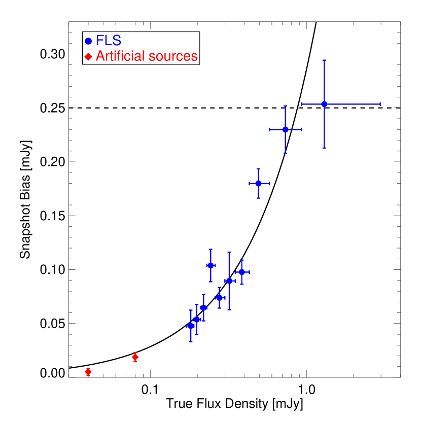
Figure 2.— Snapshot bias for stacked FIRST images as a function of the true flux density. The bias is the difference between the true flux density and the flux density measured in the median image. The sample is limited to point sources (FWHM $<2.5\arcsec$), and fitted peak values are used for the flux densities. Data are shown for both the The First-Look Survey (Condon et al. 2003; circles) and artificial 40 and 80 $\mu$Jy sources (diamonds). The vertical bars indicate $1\sigma$ errors on the stacked flux density, and the horizontal bars represent the range of flux densities for each bin. The solid line is a linear model in which the bias is 29% of the true flux density. The dashed line is the 0.25 mJy CLEAN bias measured for sources bright enough to be in the FIRST catalog.

3.3. Recovering real sub-threshold sources

An alternative to using artificial sources is to stack real radio sources detected in very deep VLA surveys. The First-Look Survey (FLS – Condon et al. 2003) covered the 5 deg² of the Spitzer First-Look fields using the VLA B configuration; it achieved a mean rms of 23 $\mu$Jy beam^-1 and detected 3565 sources down to a flux density of 115 $\mu$Jy. We ran our FIRST survey source extraction routine HAPPY (White et al. 1997) on the publicly available FLS radio images and constructed a catalog of 1445 point-like sources (deconvolved source size $<2.5\arcsec$ with the $5.0\arcsec$ beam) with flux densities ranging from 0.17 to 3.0 mJy; we chose a higher ($7\sigma$) source detection threshold to minimize the uncertainties on the individual source flux densities. We grouped the sources into ten equally populated flux density bins with mean FLS fluxes ranging from 182 $\mu$Jy to 1300 $\mu$Jy. We then extracted $1\arcmin$ cutouts around each of these sources in the FIRST images and compared the true mean flux density (from our FLS catalog) with the median stacked flux density in each bin. Source parameters were derived by fitting an elliptical Gaussian to the stacked image as described above.

We performed a similar analysis using data from the COSMOS survey’s pilot program (Schinnerer et al. 2004), comprised of seven VLA pointings in the A configuration that reached rms values ranging from 36 to 46 $\mu$Jy. The results are consistent with the FLS survey, but the uncertainties are much larger because the COSMOS sample has only one tenth as many sources as the FLS sample.

The results are displayed in Table 1 and plotted in Figure 2. For sources brighter than 0.75 mJy, the mean deficit is consistent with the 0.25 mJy CLEAN bias we have added to all above-threshold FIRST sources (see above). Below 0.75 mJy, however, the flux deficit changes character, and is well-represented by a constant fractional offset, with the stacked image yielding a value 71% that of the true mean flux density for each bin.

It is perhaps unsurprising that the bias should change near the 0.75 mJy threshold that divides brighter sources that were CLEANed during the FIRST image processing from fainter sources that have not been CLEANed. The continuity between the bias for sub-threshold sources and that for super-threshold sources suggests that they are aspects of the same phenonmenon. A connection between the bias and the depth of CLEANing is well established for brighter sources (Becker, White & Helfand 1995; Condon et al. 1998), so we think it likely (but by no means certain) that the snapshot bias is also created by the non-linear CLEAN process.

However, we are clueless as to why the relationship has the particular form we observe. According to Cornwell, Braun & Briggs (1999), “to date no one has succeeded in producing a noise analysis of CLEAN itself”, so we are not alone in being mystified. While we cannot offer a theoretical explanation for snapshot bias, we will use the simple empirical bias correction:

$$S_{p,corr}=\hbox{min}\left(1.40\,S_{p}\,,\,S_{p}+0.25\,\mbox{mJy}\right)\quad,$$ (1)

where $S_{p}$ is the fitted peak flux density measured from the median stack.

Although Eq. (1) was derived from elliptical Gaussian fits to the stacked images, we find it applies equally well if the brightness of the central pixel in the median image is used to estimate the peak flux density. We use both approaches below in the analysis of the quasar sample.

Note that it is most fortunate that the bias is a constant fraction of the flux, since that means that it can be corrected in the stacked image. That would not be true if, for example, it were a quadratic function of flux, since in that case the bias in the summed image would depend on the detailed distribution of contributing fluxes (which is unknown). But since all faint sources have the same bias correction multiplier, the bias correction can be appropriately applied to the stacked image instead of the individual images. In fact, it can be applied pixel-by-pixel to the stacked image by simply multiplying each pixel in the image by 1.40.

3.4. Stacking White Dwarfs, a Radio-Silent Population

In the remainder of the paper we discuss the results of stacking quasars divided into groups using many different parameters (redshift, optical luminosity, etc.) In all of the quasar subpopulations we stack, we always detect a positive signal. In order to allay concern that our algorithm somehow guarantees a detection, we have stacked 2,412 white dwarfs from the SDSS DR1 white dwarf catalog (Kleinman et al. 2004). As expected, the stacked image shows no hint of any source. The image rms is $3.6~{}\mbox{$\mu$Jy}$, comparable to the value expected from the typical FIRST rms of $145~{}\mbox{$\mu$Jy}$ divided by $\sqrt{N}=49$.

4. The Radio Properties of Undetected Quasars

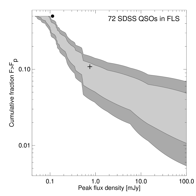
Figure 3.— The cumulative fraction of radio-detected quasars as a function of 20 cm flux density. The shaded bands represent the $\pm 1\sigma$ and $\pm 90\%$ uncertainties derived using the FLS images for the 72 SDSS quasars in the FLS survey area. The cross at 0.75 mJy represents the fraction of all SDSS quasars detected in the FIRST survey above this flux density, while the dot at 50% fraction indicates the value of the median flux density derived from our stacking analysis. The general agreement of the latter with the fraction of directly detected quasars at these flux densities offers validation of our approach, but the noise (which is comparable to the symbol size) is far smaller in the values derived from the stacked images.

Although radio emission was the defining feature of the first quasars, more than four decades of effort has failed to establish predictive models for quasar radio properties. While $\sim 10\%$ of quasars are relatively bright at centimeter wavelengths ($>1~{}\mbox{mJy}$) and thus are readily detected, the radio emission from most quasars falls well below the limits of all large-area radio surveys. Even deeper surveys that cover several square degrees of sky only detect $\sim 50\%$ of quasars. For example, by examining the images from the FLS radio survey described above (Condon et al. 2003), we detect 36 of 72 SDSS quasars to a limiting flux density of $\sim 0.09$ mJy. Figure 3 shows the fraction of detected sources as a function of flux density. The width of the shaded bands represent the $1\sigma$ and 90% confidence uncertainties; it is apparent that even this, the largest of all radio surveys to this depth, is inadequate for determining accurately the detected fraction as a function of flux density, let alone for understanding how radio emission depends on redshift, absolute magnitude, the presence of broad absorption lines, etc. For the forseeable future, 90% of quasars will remain undetected at radio wavelengths. By using image stacking with the FIRST survey, however, one can begin to quantify the statistical properties of quasar radio emission at all flux density levels.

4.1. The radio properties of SDSS quasars

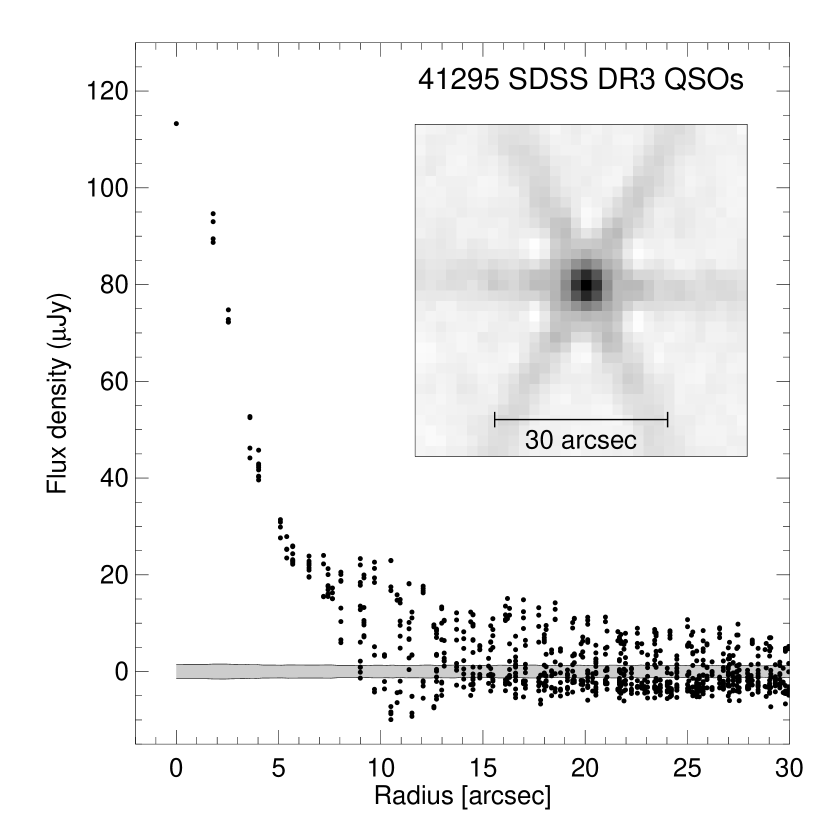
Figure 4.— The result of constructing a median stack of the 41,295 source positions in the SDSS DR3 quasar catalog. The inset displays a $1\arcmin$-square greyscale image (pixel size $1.8\arcsec$); the positive and negative sidelobes of the VLA dirty beam pattern are apparent. The pixel-by-pixel radial plot shows the “source” profile with a FWHM of $\sim 7.0\arcsec$, which is slightly extended compared with the PSF FWHM of $\sim 5.4\arcsec$. Flux density values have been corrected for snapshot bias (eqn. 1). The gray shaded band indicates the $\pm 1\sigma$ errors calculated for median statistics (Gott et al. 2001).

As a starting point we use the largest existing quasar survey as reported in the SDSS DR3 catalog (Schneider et al. 2005), which contains 46,420 spectroscopically identified quasars. Of these 41,295 fall in regions covered by the FIRST survey. Constructing a median stack of the entire sample yields the image shown as the inset in Figure 4. This high signal-to-noise ($\sim 75:1$) image shows a compact source centered on the nominal quasar(s’) position; a two-dimensional Gaussian fit yields a peak raw flux density of $80~{}\mbox{$\mu$Jy}$, or roughly 50% of the rms of an individual FIRST image. Multiplying this by 1.40 to correct for the snapshot bias (Eq. 1) gives a peak flux density of $112\pm 1.5~{}\mbox{$\mu$Jy}$. The fluxes plotted in Fig. 4 and all fluxes quoted hereafter have been corrected for the bias.

The six positive-flux radial spokes and interspersed negative features are characteristic of the VLA sidelobe pattern; since the vast majority ($\sim 93\%$) of sources contributing to this image are below the FIRST detection threshold and are therefore not CLEANed, this sidelobe pattern is expected. Note that nearly all FIRST fields are observed near the meridian so that sidelobes from different fields align well. The pixel-by-pixel radial profile in Figure 4 shows a FWHM of $\sim 7.0\arcsec$, slightly larger than the size expected for a point source observed in the VLA B configuration at 20 cm. The shaded horizontal band indicates the $\pm 1\sigma$ values derived for median statistics (Gott et al. 2001).

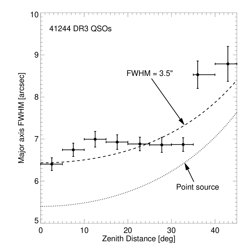
Figure 5.— Size of the major axis for the stacked quasar images as a function of the distance from the zenith at the VLA. The VLA PSF width increases with zenith distance due to foreshortening of the array in the north-south direction. The lines show the expected relationship for a point source (dotted) and for a Gaussian source having a FWHM of $3.5\arcsec$ (dashed).

The intrinsic radio source size implied by the extended emission is affected by the VLA PSF size, which depends on the distance of the source from the zenith. Since most FIRST fields were observed close to the meridian, the zenith distance is a simple function of the source declination. Figure 5 shows the measured radio sizes in image stacks separated into nine zenith-distance bins. The increase in size at high zenith distances is explained by the increase in the VLA beam size. Since the many quasars being averaged for this measurement are randomly oriented, the stacked radio image is expected to be symmetrical, and asymmetries are explained by beam effects. Both the distribution with zenith distance and the fitted size for the image in Figure 4 ($6\farcs 4\times 7\farcs 0$ FWHM) are consistent with a symmetrical quasar image having a mean source size of 3$\farcs$5. This is a bit larger than the size of quasars at the 1 mJy detection limit of the FIRST survey. Fitting the mean stack for the 679 quasars with central flux densities between 1 and 2 mJy yields a size of $5\farcs 8\times 6\farcs 2$, implying an underlying source size of $2\farcs 0\times 3\farcs 0$ when the beam size is deconvolved.

The median flux density of $\sim 110~{}\mbox{$\mu$Jy}$ is reasonably consistent with that found for the directly detected quasars within the FLS sample (Fig. 3), though it is slightly higher than the value in the FLS field ($74\pm 20~{}\mbox{$\mu$Jy}$). It is likely that this difference is mainly the result of sample variance in the FLS field. If we stack the FIRST images for only the quasars in the FLS fields, the flux density is $76\pm 26~{}\mbox{mJy}$, in good agreement with the measurement from the FLS images.

4.2. Variation of radio properties with optical luminosity

Figure 6.— The median flux density for SDSS DR3 quasars as a function of redshift.

Figure 7.— The median radio flux depends strongly on the SDSS $i$ magnitude. Note that the for the brightest quasars the median flux approaches the FIRST detection limit at 1 mJy. This is consistent with the conclusion from the FIRST Bright Quasar Survey that FIRST detects most $V\sim 15$ quasars (White et al. 2000.)

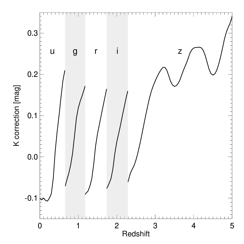
Figure 8.— $K$-correction as a function of redshift to convert observed SDSS magnitudes to the magnitude at 2500 Å rest wavelength, derived using the SDSS composite quasar spectrum (Vanden Berk et al. 2001). The $K$-correction is added to the magnitude in the SDSS filter closest to 2500 Å (shown by the vertical bands). The redshift-dependent bandwidth-stretching factor, $-2.5\log(1+z)$, has been omitted here to make the plot clearer.

Dividing the SDSS quasars into ten redshift bins, we see that the median flux density declines monotonically to $z=2$ (Fig. 6). At $z=2.25$ there is a noticeable jump in the radio flux, which is a consequence of a confluence of effects driven by the sharply declining efficiency of the SDSS quasar selection algorithm (because the colors of $z=2$–3 quasars are similar to stars; Richards et al. 2001, 2002) combined with an interesting dependence of the radio emission on optical color (discussed further below in §4.3).

The decline of flux with redshift is slower than the expected scaling as the inverse of the luminosity-distance squared because the SDSS sample is flux-limited and so detects increasingly luminous objects as the redshift increases. An interesting point is that although the FIRST catalog is also flux-limited, the stacked FIRST data are not flux-limited. All sources get included in the stack regardless of their radio brightnesses. Consequently these data do not suffer from the usual bias against faint sources in the radio; only the optical flux limit introduces such a bias. The radio luminosities are biased toward brighter values at high redshifts only insofar as the radio and optical luminosities are correlated.

The correlation between radio and optical luminosities does introduce complications in interpreting our results. Figure 7 displays the radio flux as a function of SDSS $i$-band magnitude. Optically bright sources are far more likely to be radio bright; in fact, for the brightest quasars with $i<16$, the median radio flux density approaches the 1 mJy detection limit for the FIRST survey. This is consistent with the conclusion from the FIRST Bright Quasar Survey that FIRST detects most $V\sim 15$ quasars (White et al. 2000.) But the potential entanglement of redshift, absolute magnitude, and evolution makes it difficult to understand the physical implications of this correlation.

We have concluded that the best approach is to correct for the correlation between absolute magnitude and radio luminosity before attempting to understand the variation in radio brightness with secondary parameters. We compute the 2500 Å absolute magnitude, $M_{UV}$, by applying a redshift-dependent $K$-correction derived using the Vanden Berk et al. (2001) composite SDSS quasar spectrum (Fig. 8). The $K$-correction is applied to the filter closest to 2500 Å at the quasar redshift. The observed 20 cm flux densities are converted to a rest-frame 5 GHz (6 cm) radio luminosity, $\mbox{$L_{R}$}(5\,\mbox{GHz})$, using a spectral index of $\alpha=-0.5$. The redshift is converted to luminosity distance using a standard WMAP cosmology ($\Omega_{m}=0.3$, $\Lambda=0.7$, $h=0.7$). The particular choice of rest frame wavelengths facilitates comparison of our results with previous studies using the radio-loudness parameter $R^{*}$, defined by Stocke et al. (1992) as the ratio of the 2500 Å and 5 GHz flux densities.

Figure 9.— The 5 GHz median radio luminosity $L_{R}$ is very well correlated with $M_{UV}$, the absolute ultraviolet magnitude at 2500 Å rest wavelength.

We convert each FIRST cutout image to radio luminosity units using the known quasar redshift and then stack those scaled images to compute median radio luminosities. Figure 9 shows the very close correlation between $M_{UV}$ and $L_{R}$, which is well fitted by a power-law:

$$\log\,\mbox{$L_{R}$}=0.54-0.339(\mbox{$M_{UV}$}+25)\quad,$$ (2)

where $L_{R}$ is in units of $10^{30}\,\hbox{ergs}\,\hbox{s}^{-1}\hbox{Hz}^{-1}$. If the radio luminosity were simply proportional to the optical luminosity, the slope would be steeper ($-0.4$ instead of $-0.339$). This slope implies $\mbox{$L_{R}$}\sim L_{opt}^{0.85}$; the radio loudness $R^{*}$ is a declining function of optical luminosity, with the most luminous sources ($\mbox{$M_{UV}$}=-28.5$) having $R^{*}$ values that are lower by a factor of 3 compared with the least luminous sources ($\mbox{$M_{UV}$}=-20$).

Figure 10.— The radio luminosity as a function of absolute magnitude with the quasar sample divided into redshift intervals. Only DR3 quasars selected using the primary or high-z selection criteria are included. The upper left panel shows the combined sample; the number in parentheses gives the number of sources in each redshift interval. Despite the strong absolute magnitude-redshift correlation, which can make it difficult to separate dependencies on the two variables, it is clear that the quasars in all the redshift bins follow the same $L_{R}$ versus $M_{UV}$ relationship with at most modest variations.

The absolute magnitude is strongly correlated with redshift, but if the sample is divided into redshift intervals we find that a similar $L_{R}$ versus $M_{UV}$ correlation applies at all redshifts (Fig. 10). For this test we have restricted the sample of DR3 quasars to those selected using the primary or high-z targeting criteria (Schneider et al. 2005). The primary selection used $ugri$ colors to identify quasar candidates at $z<3$ with magnitudes $i<19.1$; it includes 25,511 objects in regions covered by FIRST. The high-z criterion used $griz$ colors to identify candidates to fainter levels ($i<20.2$) and at redshifts greater than 3; our sample includes 2,412 such objects. The bulk of the remaining DR3 quasars were selected using various serendipity criteria. We exclude them here because objects so selected have unusual radio properties (as discussed further below in §4.3.)

In order to remove this strong radio-optical correlation, we scale the radio properties to the reference absolute magnitude $\mbox{$M_{UV}$}=-25$. This is accomplished simply by multiplying the FIRST cutout by an $M_{UV}$-dependent factor:

$$\log\,S_{M}=0.339(\mbox{$M_{UV}$}+25)+\log\,S\quad,$$ (3)

where $S$ is the original radio flux density. The adjustment to the radio luminosity, $L_{R,M}$, is similar, and the adjusted radio-loudness ratio is:

$$\log\,\mbox{$R^{*}_{M}$}=-0.061(\mbox{$M_{UV}$}+25)+\log\,R^{*}\quad.$$ (4)

In all cases the $M$ subscript indicates that the quantity has been adjusted for the absolute magnitude dependence.

4.3. Variation of radio properties with redshift and color

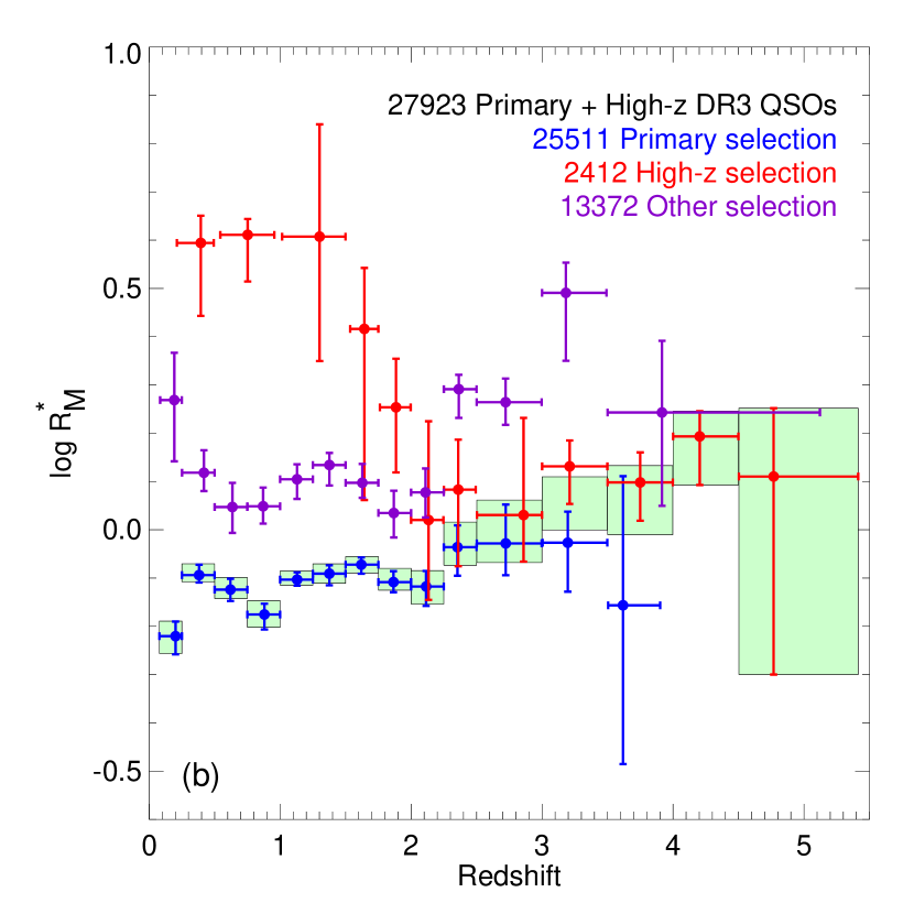
Figure 11.— The dependence of the absolute-magnitude-adjusted radio loudness $R^{*}_{M}$ on redshift. (a) The distribution for the quasars selected using the primary and high-z criteria is fairly flat, with $R^{*}_{M}$ rising by a factor of 2 between $z=0$ and $z=5$. (b) When the sample is separated using the SDSS selection criteria it is apparent that the radio properties vary greatly for different SDSS samples. The green boxes show the same combined distribution from panel (a).

Figure 12.— The absolute magnitude-adjusted radio loudness $R^{*}_{M}$ decreases toward brighter $i$ magnitudes.

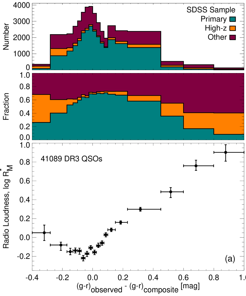
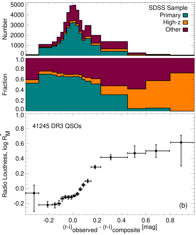
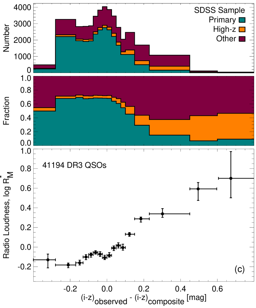
Figure 13.— Dependence of the absolute magnitude-adjusted radio loudness $R^{*}_{M}$ on the SDSS optical colors. The $x$-axis is the difference between the observed SDSS colors and those predicted for the standard SDSS composite quasar spectrum at the same redshift; the nominal color is therefore zero. The top plot shows the histogram of the number of quasars in each color bin, with quasars selected using different candidate criteria colored differently. The middle plot shows the fraction of quasars selected by the criteria in each bin; note that extreme colors are much less likely to have been selected using the primary criterion. The bottom plot displays the mean radio loudness as a function of color. Quasars that are either redder or bluer than the composite are much brighter in the radio. The three panels show to distribution for different SDSS colors ($g-r$, $r-i$, and $i-z$).

Figure 11(a) shows the redshift dependence of the radio loudness $R^{*}_{M}$ after adjusing for the dependence on absolute magnitude. There is only modest evolution in this quantity, with the radio-loudness being a factor of two higher at $z=5$ than at $z=0$. The radio properties of typical quasars have changed little since the universe was one billion years old.

The picture changes, however, if we separate the SDSS DR3 sample according to the criteria used to select the candidate quasars for spectroscopic observations (Fig. 11b). The quasars selected using the high-z criterion, which are redder and fainter than the primary candidates, are brighter in the radio. This is most noticeable at low redshifts ($z<2$), where the difference in brightness is a factor of 4. Even at high redshifts ($z>3$) a slight difference persists; at least part of the slow rise in $R^{*}_{M}$ toward higher redshifts (Fig. 11a) appears to be created by the transition in the SDSS sample from primary-dominated selection for $z<3$ to high-z-dominated selection for $z>3$.

Quasars selected using other criteria (serendipity, ROSAT, FIRST, stars, etc., as described in Schneider et al. 2005) are also systematically radio louder. One might be tempted to ascribe this to the use of the FIRST catalog in selecting some of these candidates; however, that introduces at most a very minor bias toward higher $R^{*}_{M}$ values. Only 279 of the 13,372 sources selected using other criteria are flagged in the DR3 catalog as FIRST sources, and excluding them reduces the median radio loudness only slightly from $\log\,\mbox{$R^{*}_{M}$}=0.11$ to $0.08$. (The robustness of the median to the presence of a rare admixture of bright sources is of course the reason we choose to use it.) Similarly, excluding ROSAT-selected sources — since radio emission is known to be more common among X-ray quasars (e.g., Green et al. 1995) — also leads to only a very small reduction in $R^{*}_{M}$. We conclude that there must be another explanation for the different radio properties of the variously selected quasar samples.

One possible contributor is the anti-correlation between radio loudness and apparent magnitude (Fig. 12). The optically fainter sources are radio-louder, even after the $M_{UV}$ adjustment. Quasar candidates selected using the primary criterion are on average 1 magnitude brighter than those selected using other criteria ($i=18.6$ versus 19.6). But that accounts for a difference in $\log\,\mbox{$R^{*}_{M}$}$ of only 0.15 and so does not explain the bulk of the difference between the samples.

The most important underlying correlation that leads to differences between the different SDSS samples is a strong dependence of radio loudness on optical color (Fig. 13). Since quasar colors change systematically with redshift as various emission lines move through the SDSS filters, we have subtracted the color of the SDSS composite quasar spectrum (Vanden Berk et al. 2001) from the observed colors. That reduces the scatter in colors and makes the expected color zero for a quasar that resembles the composite. We see a striking correlation: quasars that are either bluer or redder than the standard color are brighter in the radio, and substantially redder objects (with $g-r>0.8$ magnitudes) are brighter by a factor of $\sim 10$ than quasars with typical colors.

Figure 14.— Variation in the median radio flux density as a function of optical color. The composite quasar color has been subtracted from the observed SDSS $g-r$ color. Redder sources have brighter fluxes, with the reddest being $\sim 2.5$ times the typical FIRST image rms (145 $\mu$Jy).

The tendency of radio-loud quasars to have a larger scatter in their optical colors has been noted before (Richards et al. 2001, Ivezić et al. 2002), although it has never been so clearly seen as in this analysis. Not only are the red quasars radio-louder, but their median flux densities are also far higher (Fig. 14). The increase in $R^{*}_{M}$ for red objects is due primarily to brighter radio fluxes, not to fainter optical magnitudes (which might also be expected if the reddening is due to dust extinction.) Of the factor of 10 variation seen in $R^{*}_{M}$, a factor of 4 is attributable to brighter radio flux densities and a factor of 2.5 to fainter optical fluxes. Note that the reddest sources have median radio flux densities of nearly 0.4 mJy, tantalizingly close to detection by the FIRST survey.

Figure 13 also shows the distribution of colors for quasars selected using the various SDSS candidate criteria. Quasars selected using the primary criterion are much more concentrated toward the typical (zero) colors than are objects selected by either the high-z or other criteria. This makes a significant contribution to the radio-loudness differences between the various samples (Fig. 11b). The color differences between the primary and high-z samples, when folded through the correlation in Figure 13, lead to a difference in $\log\,\mbox{$R^{*}_{M}$}$ of $\sim 0.6$ between the samples for low-redshift quasars ($z<1.5$). That accounts for most of the difference between the samples seen in Figure 11(b).

The radio-color correlation also accounts for the bump seen in the flux density at $z=2.25$ (Fig. 6). The efficiency of the SDSS color selection for quasars declines sharply in the redshift range $2.4<z<3$ because the locus of normal quasar colors crosses the stellar locus in the SDSS color space (Richards et al. 2001, 2002). The SDSS DR3 catalog contains far fewer objects in this redshift range than might be expected based on the sensitivity of the survey. Moreover, the quasars that are included in the catalog are dominated by objects with unusual colors compared with the composite spectrum, since such objects do not resemble stars and so can be selected by the usual SDSS criteria. The jump in the radio flux over this redshift range is created by the selection of a larger fraction of redder quasars that have brighter radio emission than normal quasars.

The observed increase in radio emission for bluer quasars can be understood in the context of the unified model for AGN (Urry & Padovani 1995) as being due to a beamed blazar component affecting both the optical and radio emission. The brightening for redder sources could also be attributed to red optical synchrotron emission, but might instead be explained as an evolutionary effect where dusty quasars are more likely to be low-level radio emitters. This is likely to be a very useful clue to further understanding of the origins of radio emission in AGN.

4.4. The radio-loudness dichotomy

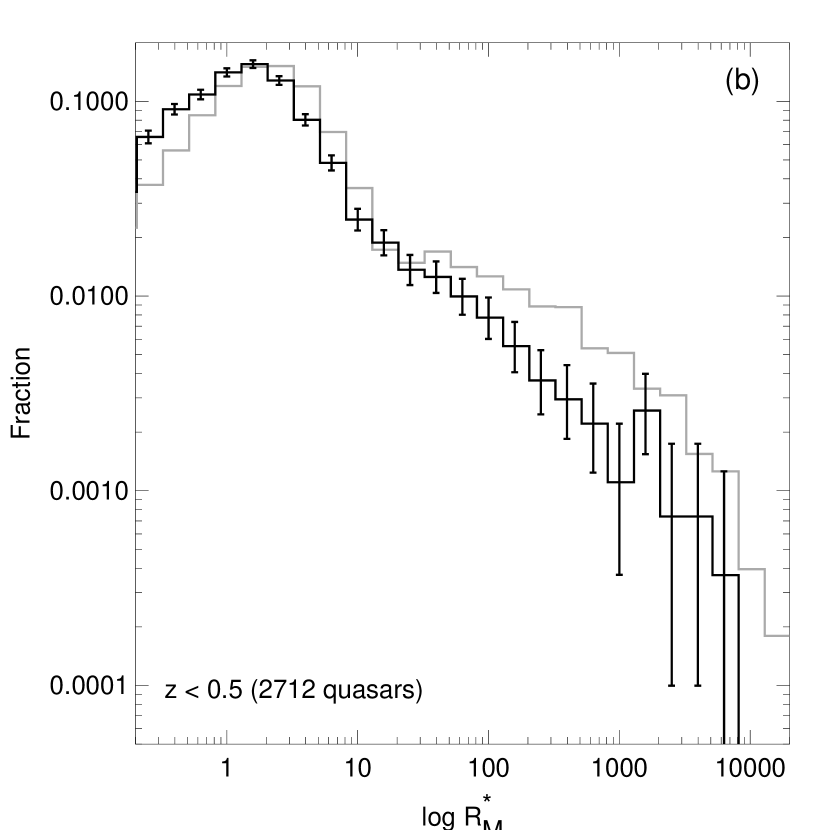
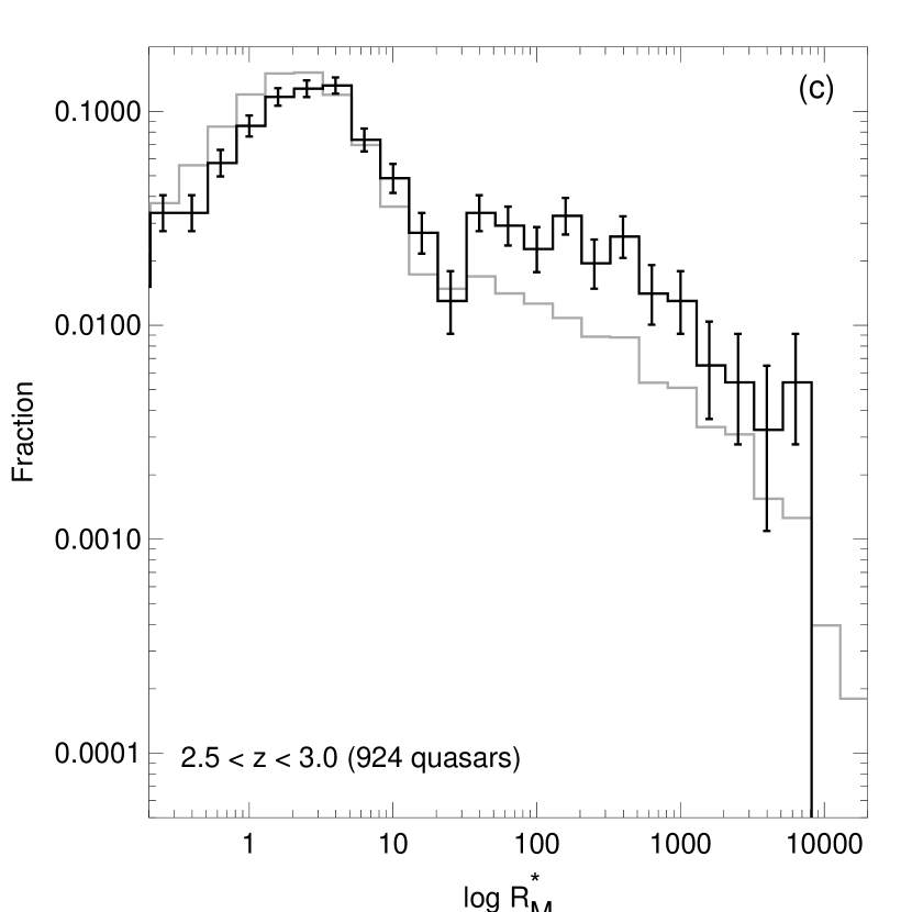
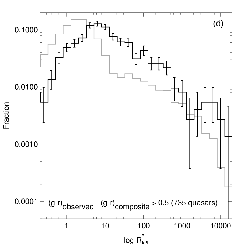
Figure 15.— The radio-loudness dichotomy as seen in the distribution of the absolute magnitude-adjusted radio loudness parameter $R^{*}_{M}$. (a) The histogram for all SDSS DR3 quasars. The inset shows an expanded view with a linear $y$ scale. There is a dip with an amplitude of $\sim 20\%$ separating radio-loud from radio-quiet objects, but the dichotomy is not so clear in different parts of parameter space. (b) Distribution for low-redshift quasars, normalized to show the fraction in each bin. The gray line shows the distribution from panel (a) for comparison. (c) Distribution for quasars in the redshift range $2.5<z<3$, where the SDSS selection effects are most severe. (d) Distribution for red quasars.

Our absolute magnitude-adjusted radio loudness parameter $R^{*}_{M}$ can be used to re-examine the issue of whether the radio loudness distribution is bimodal. While all observers agree that there is a highly non-Gaussian tail toward high $R^{*}$ values, White et al. (2000) and Cirasuolo et al. (2003a,b) did not see evidence for a truly bimodal distribution with two peaks. Ivezić et al. (2002) did find a secondary peak, though their methodology was questioned by Cirasuolo et al. Ivezić et al. (2004) subsequently applied the Cirasuolo et al. (2003b) approach to a large sample of SDSS quasar candidates and claimed conclusive evidence for a double-peaked distribution.

Figure 15 shows our distribution for the radio-loudness parameter. Note that the $R^{*}_{M}$ parameter includes both redshift-dependent $K$-corrections (as recommended by Ivezić et al. 2004) and our absolute-magnitude adjustment. The overall distribution (Fig. 15a) clearly does show a secondary peak, although the contrast in the valley between the peaks is considerably less than the factor of two found by Ivezić et al. (2004). The peak is also at a considerably lower $\log\,R^{*}$ value after the absolute magnitude adjustment ($\log\,\mbox{$R^{*}_{M}$}\sim 1.55$ instead of $\log\,R^{*}\sim 1.9$).

An exploration of the dependence of the $R^{*}_{M}$ distribution on other parameters reveals a complex situation. The radio-loud tail is considerable weaker at low redshifts ($z<0.5$; Fig. 15b) but is especially strong in the intermediate redshift range ($2.5<z<3$; Fig. 15c) where the color-section effects discussed above are dominant. For red sources, the valley disappears altogether with the resulting distribution being shifted by a factor of $\sim 3$ toward higher radio-loudness (Fig. 15c). Our conclusion is that there is indeed a double-peaked radio-loudness distribution for SDSS DR3 quasars, but that the distribution varies dramatically with redshift and color (and other parameters). The exact form of the overall distribution is likely to have been sculpted by selection effects, which must be modeled in detail before the relatively modest 20% dip between the radio-loud and radio-quiet quasars can be interpreted.

4.5. The radio emission of BAL quasars

Historically, the strongest claim associating radio properties with other quasar attributes was the absence of broad absorption lines in radio-loud quasars (Stocke et al. 1992). Becker et al. (2000) showed that some radio-loud quasars have BALs, although they noted that BALs still appeared to be absent from the most extreme radio-loud objects. Recently, Trump et al. (2006) released a catalog containing 4784 BAL and near-BAL quasars from the SDSS DR3 release. As with quasars in general, most of these objects fall below the detection threshold of FIRST, making them an ideal population for stacking studies. The FIRST survey covers 4292 of the cataloged BAL quasars.

Traditionally, BAL quasars have been divided into two primary subgroups, high ionization (HiBALs) and low ionization (LoBALs). The latter are much rarer; in the SDSS/FIRST sample there are 3647 HiBALs and only 645 LoBALs. The HiBALs are identified primarily on the basis of C IV absorption at 1550 Å, while the LoBALs are identified primarily from Mg II absorption at 2800 Å. As a result, the known LoBALs tend to be at lower redshifts than the known HiBALs. HiBALs can only be identified at redshifts $z>1.7$, while LoBALs can be recognized at redshifts as low as 0.5.

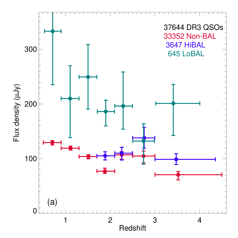
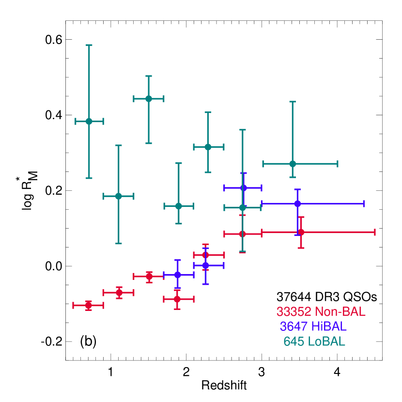
Figure 16.— Median radio flux density (left) and absolute magnitude-adjusted radio-loudness (right) for HiBAL, LoBAL and non-BAL quasars as a function of redshift. Surprisingly, BAL quasars are brighter radio sources than non-BALs, with the effect especially noticeable for low-ionization BALs.

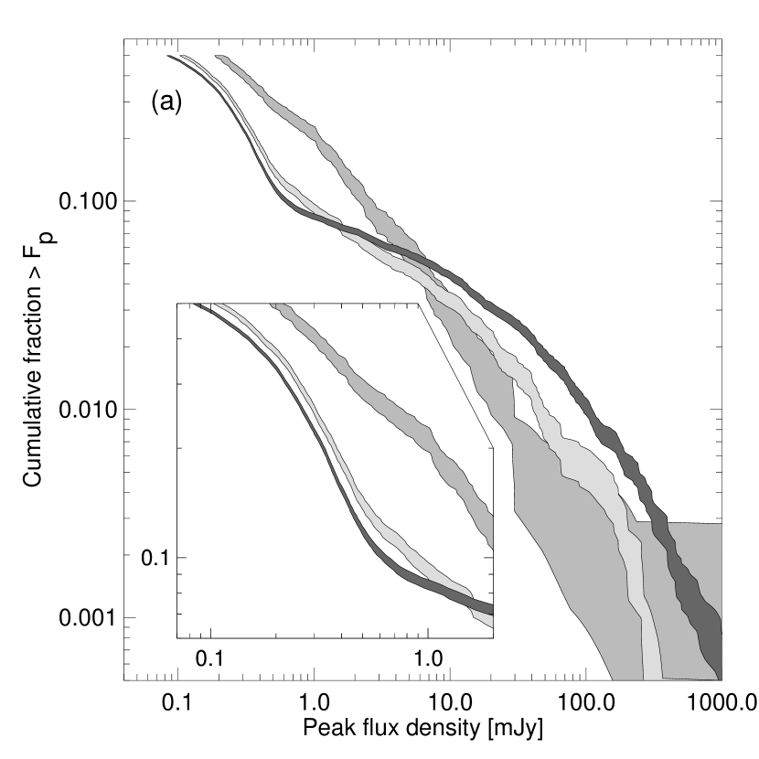
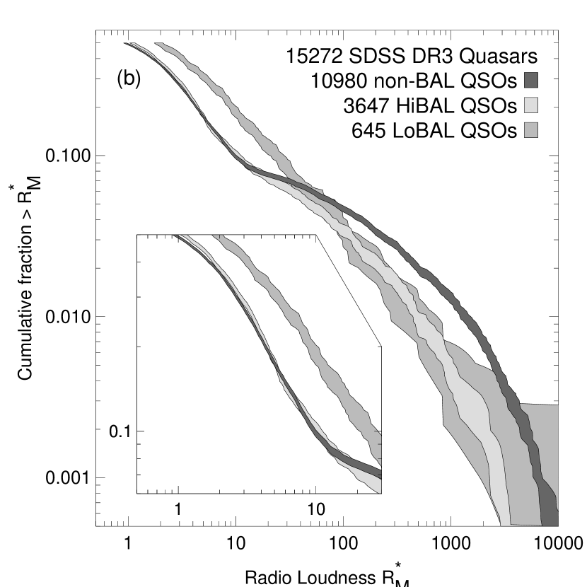
Figure 17.— The cumulative distribution of HiBAL, LoBAL, and non-BAL quasars as a function of flux density limit (left) and magnitude-adjusted radio loudness $R^{*}_{M}$ (right). The shaded bands show $1\sigma$ uncertainties. The bands converge at fraction 0.5 to the median values derived from our stacking analysis; the inset shows an expanded view of that region. There is a deficit of BAL quasars at bright fluxes, but there is an excess at fluxes fainter than $\sim 1.5$ mJy for HiBALs and $\sim 5$ mJy for LoBALs. The radio-loudness distribution is similar for non-BALs and HiBALs in the radio-intermediate region ($2<\mbox{$R^{*}_{M}$}<10$), though a small but significant difference remains for radio-quiet ($\mbox{$R^{*}_{M}$}<2$) sources. The LoBALs are much more likely to be radio-intermediate sources than either the HiBALs or non-BALs.

In Figure 16(a), we show the median radio flux density of HiBALs, LoBALs, and non-BALs as a function of redshift. Interestingly, both classes of BAL quasars are brighter in the radio than non-BALs. The absolute-magnitude-adjusted radio loudness $R^{*}_{M}$ shows a similar effect (Fig. 16b), indicating that this is not due to a difference in the distribution of $M_{UV}$ for the various classes. The LoBALs are radio-louder by a factor $2.23\pm 0.10$ (averaged over $0.5<z<4$) and the HiBALs by a factor $1.18\pm 0.07$ ($1.7<z<4.3$).

That said, the comparison to the FIRST survey for this new large sample of BAL quasars confirms the absence of extremely radio-loud BAL QSOs. In Figure 17(a), we show the cumulative distribution of BAL and non-BAL quasars as a function of radio flux density. This plot includes only non-BALs with $1.7<z<4$, since outside that redshift range the absorption lines required for confident identification of non-BALs do not fall in the SDSS spectrum window. It is clear from the graph that while BALs are not found among the brightest radio-emitting quasars, below 2 mJy they are systematically brighter than non-BAL objects.

The disparity remains if we examine the radio-loudness parameter instead of the flux density (Fig. 17b), although the intermediate brightness HiBALs and non-BALs have $R^{*}_{M}$ distributions that are much more similar than their flux distributions. A two-sided Kolmogorov-Smirnov test shows the $R^{*}_{M}$ distributions for HiBALs and non-BALs in Figure 17(b) are different at the $4\times 10^{-5}$ level of significance. Separate tests for the distribution with $\mbox{$R^{*}_{M}$}>14$ and the portion with $\mbox{$R^{*}_{M}$}<5.25$ show that the bright and faint distributions are both discrepant ($2\times 10^{-7}$ and $4\times 10^{-6}$, respectively). The differences compared with the LoBAL distribution also highly significant ($<4\times 10^{-3}$) despite the fact that the LoBAL sample is much smaller. The $R^{*}_{M}$ distributions for the radio-bright ($\mbox{$R^{*}_{M}$}>100$) HiBAL and LoBAL quasars are statistically indistinguishible.

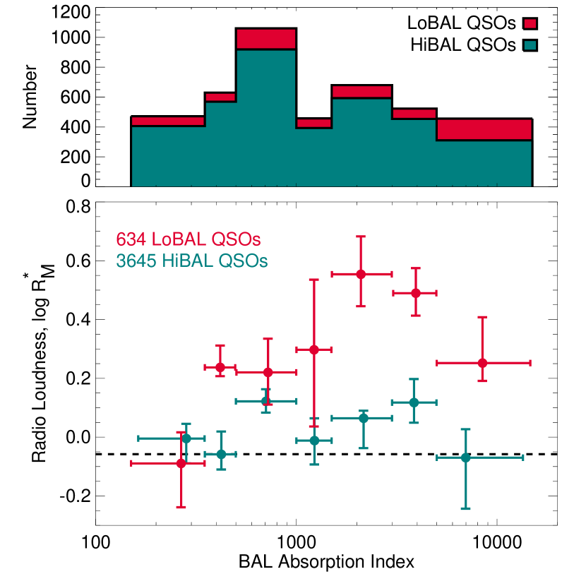
Figure 18.— Median radio-loudness for HiBAL and LoBAL quasars as a function of the BAL absorption index. The top panel shows the distribution of the absorption index values for the two types of BALs. The dashed line shows the radio loudness for the non-BAL quasars (which by definition have absorption indices of zero.) There is some indication of a drop in radio loudness for low absorption indices, although the effect is not strong.

We have also examined the dependence of $R^{*}_{M}$ on the BAL quasar catalog’s absorption index, which quantifies the strength and extent of the broad absorption (Trump et al. 2006). There is a hint of a decline in $R^{*}_{M}$ at the lowest absorption index values, though the size of the effect is modest at best (Fig. 18).

Figure 19.— Fraction of DR3 quasars that are BALs as function of redshift. HiBALs can only be recognized when $z>1.7$, which accounts for the large jump at that redshift; lower redshift quasars are all of the rare LoBAL type. The spike at $z=2.7$ is created by the inefficiency of the SDSS quasar color selection where the quasar locus passes close to the stellar locus.

We note in passing that the sample of BAL quasars in the SDSS DR3 catalog is strongly biased around $z\sim 2.5$ by selection effects that favor the discovery of objects with unusual colors. Figure 19 shows the fraction of BAL quasars as a function of redshift. For $2.7<z<2.9$, almost half the objects in the DR3 catalog are BALs! The effect here is similar to the bias in favor of the discovery of red quasars in this same redshift interval (discussed in §4.3). If the broad absorption lines change the quasar magnitude in even one of the five SDSS filter bands, it is more likely to be recognized as having colors inconsistent with the stellar locus. This effect has been previously discussed by Hewett & Foltz (2003) and Reichard et al. (2003).

We find the radio dominance of BAL over non-BAL quasars difficult to reconcile with claims that BALs are largely the result of a preferred orientation (e.g., Murray et al. 1995, Elvis 2000). In fact, most of the arguments against the orientation model to date have been based on radio observations. Zhou et al. (2006) argued that radio variability observed in six BAL QSOs was strong evidence that at least for some BALs, we were looking along the axis of the radio jet. Becker et al. (1997) made similar arguments on the basis of the flat radio spectra observed for some BAL quasars. And Gregg et al. (2006) used the FR2 radio morphology exhibited by some BAL QSOs to argue against the need of a special orientation.

If the presence of BALs is determined by orientation, the greater radio-loudness of BAL QSOs implies that we are looking closer to, not farther from, the jet axis in quasars with BALs. We know of no model that results in higher measured radio flux density from the quasar core with greater angular distance from the jet direction. Rather, relativistic beaming should enhance radio emission at small angles to the quasar symmetry axis. This is at odds with conventional orientation models that require viewing angles closer to edge-on for BAL quasars (e.g., Elvis 2000).

An alternative explanation is that quasars with low-level radio emission in the nucleus have more BAL clouds and consequently are more likely to show absorption. BAL quasars may be in a special evolutionary phase in which low-level radio emission confined near the nucleus is accompanied by an excess of absorption clouds; when the radio source breaks out to become truly radio-loud, it quickly eliminates the clouds that are the source of broad absorption lines. This is an evolutionary unification model (e.g., Lípari & Terlevich 2006).

Richards et al. (2004) and Richards (2006) suggest that the sequence from LoBALs to HiBALs to non-BALs may be the result of orientation coupled with a gradual transition from a radiation-dominated, accretion-disk wind to a MHD-dominated wind (Everett et al. 2001; Everett 2005). In this view, powerful radio-bright quasars have a tightly collimated polar MHD wind in which BAL clouds have a small covering factor, while radio-weak objects have more widely distributed BAL clouds in an equatorial, radiatively accelerated wind coming off the surface of the disk (see Fig. 5 of Richards et al. 2004). This is a static unification model in which the magnetic field strength (with an associated radio source) acts as a second parameter (in addition to orientation).

This picture does not necessarily predict enhanced low-level radio emission from BAL quasars since it nominally produces monotonically decreasing radio emission with increasing BAL strength. However, it could plausibly be modified to explain our observations. A weak radio source might elevate the disk wind above the equatorial plane, increasing the BAL covering factor for lines of sight that are not heavily absorbed by the disk, while a stronger radio source would collimate the flow and reduce the BAL covering fraction. Any model that matches our observations will share this non-monotonic behavior in order to produce BALs that are enhanced in the presence of low-level radio emission but suppressed by bright radio emission.

5. Summary and conclusions

We have demonstrated that the average radio properties of sources in the FIRST survey area can be derived even for populations in which the individual members have flux densities an order of magnitude or more below the typical field rms. Our median stacking algorithm is robust, and, following the calibration of snapshot bias derived herein, can be used to provide quantitative information of average source flux densities into the nanoJansky regime. In our application of this algorithm to the SDSS DR3 quasar catalog, we establish the radio properties of quasars as a function of optical luminosity, color and redshift. The average radio luminosity correlates very well with the optical luminosity, with $\mbox{$L_{R}$}\sim L_{opt}^{0.85}$. There is a very strong correlation between radio loudness and color, with quasars having either bluer or redder colors than the norm being brighter in the radio; objects 0.8 magnitudes redder than average in $g-r$ have radio loudness values 10 times higher than quasars with typical colors. At faint flux densities, BAL quasars actually have higher average radio luminosities and radio-loudness parameters than non-BAL objects, a result inconsistent with the conventional orientation hypothesis for BAL quasars.

The correlation between radio emission and color is an intriguing clue to the nature of our FIRST-selected red quasars (Gregg et al. 2002, White et al. 2003, Glikman et al. 2004a). It suggests that a wide-area radio survey only a factor of two deeper than the FIRST survey might be capable of detecting the bulk of the reddened population, which would shed light on the still controversial question of what fraction of all quasars are highly reddened.

The success of stacking FIRST images to find the mean radio properties of sub-threshold radio sources depends on the availability of large target lists. As shown in this paper, the SDSS quasar sample is ideal for these purposes. In fact the SDSS provides much more than quasars. We are currently working on a study of the mean radio properties of SDSS narrow-line AGN (deVries et al., in preparation). In that paper, we explore the dependence of radio emission on the strength of various emission lines, on associated star formation, and on black hole mass. We are also examining the radio properties of star-forming galaxies taken from the SDSS spectroscopic survey of galaxies (Becker et al., in preparation). There is no reason that these studies must be limited to extragalactic samples. Other astrophysical sources of weak radio emission include several classes of stars. (We show in §3.4 that the average radio flux density of white dwarfs is fainter than $\sim 10~{}\mbox{$\mu$Jy}$.) The number of stars with spectral classification is large enough that it will be feasible to study the radio properties as a function of spectral type.

References

- Bartelmann & White (2003) Bartelmann, M., & White, S. D. M. 2003, A&A, 407, 845
- Becker et al. (1995) Becker, R. H., White, R. L., & Helfand, D. J. 1995, ApJ, 450, 559
- Becker et al. (1997) Becker, R. H., Gregg, M. D., Hook, I. M., McMahon, R. G., White, R. L., & Helfand, D. J. 1997, ApJ, 479, L93
- Becker et al. (2000) Becker, R. H., White, R. L., Gregg, M. D., Brotherton, M. S., Laurent-Muehleisen, S. A., & Arav, N. 2000, ApJ, 538, 72
- Brandt et al. (2001a) Brandt, W. N., et al. 2001a, AJ, 122, 1
- Brandt et al. (2001b) Brandt, W. N., Hornschemeier, A. E., Schneider, D. P., Alexander, D. M., Bauer, F. E., Garmire, G. P., & Vignali, C. 2001b, ApJ, 558, L5
- Caillault & Helfand (1985) Caillault, J.-P., & Helfand, D. J. 1985, ApJ, 289, 279
- Cirasuolo et al. (2003a) Cirasuolo, M., Magliocchetti, M., Celotti, A., & Danese, L. 2003a, MNRAS, 341, 993
- Cirasuolo et al. (2003b) Cirasuolo, M., Celotti, A., Magliocchetti, M., & Danese, L. 2003b, MNRAS, 346, 447
- Clark (1980) Clark, B. G. 1980, A&A, 89, 377
- Condon et al. (1998) Condon, J. J., Cotton, W. D., Greisen, E. W., Yin, Q. F., Perley, R. A., Taylor, G. B., & Broderick, J. J. 1998, AJ, 115, 1693
- Condon et al. (2003) Condon, J. J., Cotton, W. D., Yin, Q. F., Shupe, D. L., Storrie-Lombardi, L. J., Helou, G., Soifer, B. T., & Werner, M. W. 2003, AJ, 125, 2411
- Cornwell et al. (1999) Cornwell, T., Braun, R., & Briggs, D. S. 1999, ASP Conf. Ser. 180: Synthesis Imaging in Radio Astronomy II, 180, 151
- Croom et al. (2004) Croom, S. M., Smith, R. J., Boyle, B. J., Shanks, T., Miller, L., Outram, P. J., & Loaring, N. S. 2004, MNRAS, 349, 1397
- Elvis (2000) Elvis, M. 2000, ApJ, 545, 63
- Everett et al. (2001) Everett, J. E., Königl, A., & Kartje, J. F. 2001, ASP Conf. Ser. 224: Probing the Physics of Active Galactic Nuclei, 224, 441
- Everett (2005) Everett, J. E. 2005, ApJ, 631, 689
- Glikman et al. (2004a) Glikman, E., Gregg, M. D., Lacy, M., Helfand, D. J., Becker, R. H., & White, R. L. 2004a, ApJ, 607, 60
- Glikman et al. (2004b) Glikman, E., Helfand, D., Becker, R., & White, R. 2004b, ASP Conf. Ser. 311: AGN Physics with the Sloan Digital Sky Survey, 311, 351
- Georgakakis et al. (2003) Georgakakis, A., Hopkins, A. M., Sullivan, M., Afonso, J., Georgantopoulos, I., Mobasher, B., & Cram, L. E. 2003, MNRAS, 345, 939
- Gott et al. (2001) Gott, J. R. I., Vogeley, M. S., Podariu, S., & Ratra, B. 2001, ApJ, 549, 1
- Green et al. (1995) Green, P. J., et al. 1995, ApJ, 450, 51
- Gregg et al. (2002) Gregg, M. D., Lacy, M., White, R. L., Glikman, E., Helfand, D., Becker, R. H., & Brotherton, M. S. 2002, ApJ, 564, 133
- Gregg et al. (2006) Gregg, M. D., Becker, R. H., & de Vries, W. 2006, ApJ, 641, 210
- Hewett & Foltz (2003) Hewett, P. C., & Foltz, C. B. 2003, AJ, 125, 1784
- Högbom (1974) Högbom, J. A. 1974, A&AS, 15, 417
- Hogg et al. (1997) Hogg, D. W., Neugebauer, G., Armus, L., Matthews, K., Pahre, M. A., Soier, B. T., & Weinberger, A. J. 1997, AJ, 113, 474
- Ivezić et al. (2002) Ivezić, Ž., et al. 2002, AJ, 124, 2364
- Ivezić et al. (2004) Ivezić, Z., et al. 2004, ASP Conf. Ser. 311: AGN Physics with the Sloan Digital Sky Survey, 311, 347
- Kleinman et al. (2004) Kleinman, S. J., et al. 2004, ApJ, 607, 426
- Lin et al. (2004) Lin, Y.-T., Mohr, J. J., & Stanford, S. A. 2004, ApJ, 610, 745
- Lípari & Terlevich (2006) Lípari, S. L., & Terlevich, R. J. 2006, MNRAS, 368, 1001
- Minchin et al. (2003) Minchin, R. F., et al. 2003, MNRAS, 346, 787
- Murray et al. (1995) Murray, N., Chiang, J., Grossman, S. A., & Voit, G. M. 1995, ApJ, 451, 498
- Reichard et al. (2003) Reichard, T. A., et al. 2003, AJ, 126, 2594
- Richards et al. (2001) Richards, G. T., et al. 2001, AJ, 121, 2308
- Richards et al. (2002) Richards, G. T., et al. 2002, AJ, 123, 2945
- Richards et al. (2004) Richards, G., Hall, P., Reichard, T., vanden Berk, D., Schneider, D., & Strauss, M. 2004, ASP Conf. Ser. 311: AGN Physics with the Sloan Digital Sky Survey, 311, 25
- Richards (2006) Richards, G. T. 2006, ArXiv Astrophysics e-prints, arXiv:astro-ph/0603827
- Scaramella et al. (1993) Scaramella, R., Cen, R., & Ostriker, J. P. 1993, ApJ, 416, 399
- Schneider et al. (2005) Schneider, D. P., et al. 2005, AJ, 130, 367
- Serjeant et al. (2004) Serjeant, S., et al. 2004, ApJS, 154, 118
- Schinnerer et al. (2004) Schinnerer, E., et al. 2004, AJ, 128, 1974
- Stocke et al. (1992) Stocke, J. T., Morris, S. L., Weymann, R. J., & Foltz, C. B. 1992, ApJ, 396, 487
- Trump et al. (2006) Trump, J. R., et al. 2006, ApJS, 165, 1
- Urry & Padovani (1995) Urry, C. M., & Padovani, P. 1995, PASP, 107, 803
- Vanden Berk et al. (2001) Vanden Berk, D. E., et al. 2001, AJ, 122, 549
- Wals et al. (2005) Wals, M., Boyle, B. J., Croom, S. M., Miller, L., Smith, R., Shanks, T., & Outram, P. 2005, MNRAS, 360, 453
- White et al. (1997) White, R. L., Becker, R. H., Helfand, D. J., & Gregg, M. D. 1997, ApJ, 475, 479
- White et al. (2000) White, R. L., et al. 2000, ApJS, 126, 133
- White et al. (2003) White, R. L., Helfand, D. J., Becker, R. H., Gregg, M. D., Postman, M., Lauer, T. R., & Oegerle, W. 2003, AJ, 126, 706
- Windhorst et al. (1993) Windhorst, R. A., Fomalont, E. B., Partridge, R. B., & Lowenthal, J. D. 1993, ApJ, 405, 498
- Zhou et al. (2006) Zhou, H., Wang, T., Wang, H., Wang, J., Yuan, W., & Lu, Y. 2006, ApJ, 639, 716
- Zibetti et al. (2005) Zibetti, S., White, S. D. M., Schneider, D. P., & Brinkmann, J. 2005, MNRAS, 358, 949