The nature and evolution of the highly ionized near-zones in the absorption spectra of $z\simeq 6$ quasars

Abstract

We use state-of-the-art hydrodynamical simulations combined with a $1$D radiative transfer code to assess the extent to which the highly ionized regions observed close to $z\simeq 6$ quasars, which we refer to as near-zones, can constrain the ionization state of the surrounding IGM. We find the appearance in Ly$\alpha$ absorption of a quasar H $\rm\scriptstyle II\$ionization front expanding into a neutral IGM can be very similar to a classical proximity zone, produced by the enhancement in ionizing flux close to a quasar embedded in a highly ionized IGM. The observed sizes of these highly ionized near-zones and their redshift evolution can be reproduced for a wide range of IGM neutral hydrogen fractions for plausible values of the luminosity and lifetime of the quasars. The observed near-zone sizes at the highest observed redshifts are equally consistent with a significantly neutral and a highly ionized surrounding IGM. Stronger constraints on the IGM neutral hydrogen fraction can be obtained by considering the relative size of the near-zones in the Ly$\alpha$ and Ly$\beta$ regions of a quasar spectrum. A large sample of high quality quasar absorption spectra with accurate determinations of near-zone sizes and their redshift evolution in both the Ly$\alpha$ and Ly$\beta$ regions should confirm or exclude the possibility that the Universe is predominantly neutral at the highest observed redshifts. The width of the discrete absorption features in these near-zones will contain important additional information on the ionization state and the previous thermal history of the IGM at these redshifts.

1 Introduction

Unravelling the epoch of hydrogen reionization is one of the major remaining goals of observational cosmology. The discovery of extended high opacity regions in the absorption spectra of $z\ga 6$ quasars has provoked an intense discussion as to whether or not the tail end of the reionization epoch has been detected. Following the three year WMAP results, the complementary constraints on the start and duration of the reionization epoch from cosmic microwave background data are now actually very weak (Page et al. 2006; Spergel et al. 2006). An extended period of reionization starting at $z\sim 15$ and a rather rapid reionization around $z\sim 6$ both appear to be consistent with the data. Much hope for further progress is based on upcoming experiments to detect high-redshift $21\rm~{}cm$ emission/absorption (Scott & Rees 1990; Madau et al. 1997; Shaver et al. 1999; Tozzi et al. 2000). Currently, however, the study of Lyman series absorption in the spectra of quasars (Fan et al. 2002; Fan et al. 2006b) and gamma-ray bursts (Ciardi & Loeb 2000; Barkana & Loeb 2004; Totani et al. 2006) are the key observational probe of the hydrogen reionization epoch. The absence of a Gunn-Peterson trough (Gunn & Peterson 1965) in quasar spectra at $z<5.5$ shows unambiguously that the volume weighted neutral hydrogen fraction in the intergalactic medium (IGM) is less than one part in $10^{4}$ (Fan et al. 2002; Fan et al. 2006b). Hydrogen reionization is therefore definitely complete at this time. However, at $z\simeq 6$ the detection of dark absorption troughs in quasar spectra indicates the IGM neutral hydrogen fraction is increasing rapidly with look back time (Djorgovski et al. 2001; Becker et al. 2001; Songaila & Cowie 2002; Pentericci et al. 2002; White et al. 2003; Fan et al. 2006b). Whether a large fraction of the volume is still neutral at this time is, however, rather controversial. Fan et al. (2006b) obtain a lower limit on the volume weighted neutral hydrogen fraction of $f_{\rm HI}\geq 10^{-3.5}$ at $z\geq 6$ from a detailed analysis of the Lyman series absorption in quasar spectra. There are also claims for an acceleration in the upwards evolution of the Ly$\alpha$ optical depth at $z\simeq 6$ (Cen & McDonald 2002; Fan et al. 2002; White et al. 2003; Fan et al. 2006b) which may occur during the epoch when individual H $\rm\scriptstyle II\$regions overlap (Gnedin 2000, 2004). Other authors, however, argue that the data is consistent with a smooth evolution due to the gradual thickening of the Ly$\alpha$ forest (Songaila 2004; Becker et al. 2006). Large variations in the transmitted flux along different lines-of-sight further complicate the picture. Large Lyman series troughs are detected in several quasar spectra at $z\simeq 6$ (Fan et al. 2006b). Yet the spectrum of $\rm J1148+5251$ at $z=6.42$ exhibits patchy transmission, indicating the IGM is highly ionized in at least some locations (White et al. 2003, 2005; Oh & Furlanetto 2005). This may be indicative of spatial fluctuations in the UV background which are expected at the end of reionization (Wyithe & Loeb 2006; Fan et al. 2006b), but may also be attributed to the fluctuations of the IGM density alone (Lidz et al. 2006; Liu et al. 2006). It is thus currently unclear whether the IGM is highly ionized, substantially neutral or indeed a combination of both just above $z=6$, depending on the line-of-sight considered. Answering this question conclusively will have important implications for the nature of hydrogen reionization.

The main limitation of Lyman series absorption as a probe of the IGM neutral hydrogen fraction is it ceases to be sensitive at $f_{\rm HI}\ga 10^{-3}$. Other approaches to probing the IGM neutral hydrogen fraction at $z\geq 6$ include analysing metal absorption systems (Oh 2002; Furlanetto & Loeb 2003; Becker et al. 2006b), the luminosity function of Ly$\alpha$ emitting galaxies (Malhotra & Rhoads 2004; Hu et al. 2005; Kashikawa et al. 2006), and the dark gap width distribution (Paschos & Norman 2005; Gallerani et al. 2006) although all have their associated interpretative uncertainties (see Fan et al. 2006a for an recent review of results from all these techniques).

In this work we shall concentrate on yet another probe of the neutral hydrogen fraction of the high-redshift IGM. Recently, claims that the IGM has a large neutral hydrogen fraction at $z>6$ have been made based on the observed sizes of the small regions of transmitted flux observed in quasar absorption spectra just blue-ward of the quasar’s redshift (Wyithe & Loeb 2004; Mesinger & Haiman 2004; Mesinger et al. 2004; Wyithe et al. 2005; Yu & Lu 2005). In the regions close to the quasar intergalactic hydrogen is expected to be highly ionized. The typical sizes of these regions observed in Ly$\alpha$ absorption at $z\simeq 6$ are $5-10$ proper Mpc (Fan et al. 2006b). Throughout this paper we shall refer to these regions as near-zones. This accounts for the possibility that these regions may be either the observational signature of quasar H $\rm\scriptstyle II\$ionization fronts expanding into a significantly neutral IGM, or classical proximity zones due to enhanced ionizing flux near the quasar (Bajtlik et al. 1988).

Wyithe et al. (2005) use the size of spectroscopically identified near-zones observed around seven quasars at $6\leq z\leq 6.42$ to infer $f_{\rm HI}\geq 0.1$. An alternative analysis by Mesinger & Haiman (2004) uses the difference between the sizes of the near-zones identified in the Ly$\alpha$ and Ly$\beta$ regions of the spectrum of a single quasar at $z=6.28$ to obtain $f_{\rm HI}\geq 0.2$. They attribute the slightly smaller size of the Ly$\alpha$ near-zone to the presence of a damping wing from a significantly neutral IGM (Miralda-Escudé & Rees 1998; Miralda-Escudé 1998). If these results are correct, they would imply a very rapid increase in the neutral hydrogen fraction over a short redshift interval, from $f_{\rm HI}\sim 10^{-4}$ at $z=5.5$ to $f_{\rm HI}\geq 10^{-1}$ at $z\sim 6.4$. In contrast, by comparing the relative sizes of Ly$\alpha$ near-zones observed around $16$ quasars, Fan et al. (2006b) conclude the IGM neutral hydrogen fraction increases by a factor of $\sim 14$ assuming the near-zone sizes scale as $(1+z)^{-1}f_{\rm HI}^{-1/3}$ over the same redshift range. They find no strong evidence for a significantly neutral IGM at $z=6.4$.

These results appear to be in direct contradiction with each other. However, there are a number of uncertainties which may explain the origin of these different conclusions. Using the properties of spectroscopically identified near-zones to determine the IGM neutral hydrogen fraction requires assumptions about the ionizing luminosity and lifetime of quasars, as well as the density distribution of the surrounding IGM. The clumpy nature of the IGM will produce large variations in near-zone sizes from one line-of-sight to the next, with the underdense regions in the IGM setting the observed sizes of these regions (e.g. Oh & Furlanetto 2005). Further uncertainties arise from the possibility of fainter ionizing sources clustered around the quasar and the exact details of the radiative transfer through the inhomogeneous IGM. The sizes of the spectroscopically identified near-zones themselves are also uncertain. They are determined from generally noisy, moderate or low resolution spectra and the systemic redshift of the quasar is usually not known to a high degree of accuracy. It is also not immediately clear whether the observed sizes of near-zones correspond to the full extent of the regions impacted by the ionizing radiation of the quasars (i.e. the region behind the quasar H $\rm\scriptstyle II\$ionization front), a key assumption when inferring the IGM neutral hydrogen fraction from the sizes of near-zones.

In this paper we investigate these issues in some detail. We model highly ionized Ly$\alpha$ and Ly$\beta$ near-zones around high redshift quasars using a large hydrodynamical simulation combined with an accurate scheme for radiative transfer through an inhomogeneous IGM of primordial composition. We shall consider the information one may realistically infer about the ionization state of the IGM from the observed sizes of Lyman series near-zones. In section 2 we develop a simple analytical model for the sizes of the spectroscopically observed near-zones. A brief overview of our radiative transfer simulations is presented in section 3, and in section 4 we examine the dependence of Ly$\alpha$ and Ly$\beta$ near-zones sizes on the IGM neutral hydrogen fraction, quasar age and ionizing photon production rate. We consider the evolution in Ly$\alpha$ near-zone sizes observed by Fan et al. (2006b) in section 5 and present our conclusions in section 6. Details of our radiative transfer implementation and treatment of unresolved self shielded clumps are found in the appendices.

Throughout this paper we adopt the following set of cosmological parameters $(\Omega_{\rm m},\Omega_{\Lambda},\Omega_{\rm b}h^{2},h,\sigma_{8},n)=(0.26,0.74,0.024,0.72,0.85,0.95)$, consistent with the combined analysis of three year WMAP and Ly$\alpha$ forest data (Viel et al. 2006; Seljak et al. 2006), and a helium fraction by mass of $Y=0.24$ (e.g. Olive & Skillman 2004). Unless otherwise stated all distances referred to in the text correspond to proper distances.

2 H $\rm\scriptstyle II\$ionization fronts and the proximity effect

2.1 The extent of the regions impacted by quasar ionizing radiation

We firstly consider the case of an H $\rm\scriptstyle II\$ionization front (I-front) expanding into a significantly neutral IGM. Consider the idealised case of an observer positioned along the line of sight to a monochromatic ionizing source, isotropically emitting $\dot{N}$ Lyman limit photons per unit time into a homogeneous, pure hydrogen IGM with a volume weighted neutral hydrogen fraction $f_{\rm HI}=n_{\rm HI}/n_{\rm H}$. If this observer could measure the exact size of the H $\rm\scriptstyle II\$region around the source at various times $t$ during the source lifetime, the H $\rm\scriptstyle II\$region expansion rate would be described by (see appendix A for details)

$$\frac{dR_{\rm ion}}{dt}=\frac{\dot{N}-\frac{4}{3}\pi R_{\rm ion}^{3}\alpha_{\rm HII}n_{\rm H}^{2}}{4\pi R_{\rm ion}^{2}f_{\rm HI}n_{\rm H}},$$ (1)

where $R_{\rm ion}$ is the distance of the H $\rm\scriptstyle II\$I-front from the source, $\alpha_{\rm HII}$ is the recombination coefficient for ionized hydrogen and $n_{\rm H}$ is the proper hydrogen number density at a fixed baryonic density normalised by the cosmic mean, $\Delta=\rho_{\rm b}/\bar{\rho}_{\rm b}$,

$$n_{\rm H}=7.0\times 10^{-5}\Delta\left(\frac{1+z}{7}\right)^{3}\rm~{}cm^{-3}.$$ (2)

For small values of $f_{\rm HI}$ the “I-front” obviously produces only a very small change in the ionized hydrogen fraction within a region of radius $R_{\rm ion}$.

Solving equation (1) for a source with age $t_{\rm Q}$ yields,

$$R_{\rm ion}=R_{\rm S}\left[1-\exp\left(-\frac{t_{\rm Q}}{f_{\rm HI}t_{\rm rec}}\right)\right]^{1/3},$$ (3)

where $R_{\rm S}$ is the Strömgren radius, defined as

$$R_{\rm S}=\left(\frac{3\dot{N}}{4\pi\alpha_{\rm HII}n_{\rm H}^{2}}\right)^{1/3},$$ (4)

and $t_{\rm rec}=(n_{\rm H}\alpha_{\rm HII})^{-1}$ is the recombination timescale. If $t_{\rm Q}\ll f_{\rm HI}t_{\rm rec}$ the solution to equation (1) may be rewritten as

$$R_{\rm ion}=\frac{4.2}{(\Delta f_{\rm HI})^{1/3}}\left(\frac{\dot{N}}{2\times 10^{57}\rm~{}s^{-1}}\right)^{1/3}\left(\frac{t_{\rm Q}}{10^{7}\rm~{}yrs}\right)^{1/3}$$

$$\hskip 19.91692pt\times\left(\frac{1+z}{7}\right)^{-1}\rm~{}Mpc,$$ (5)

where we have adopted some fiducial values for a quasar embedded in a uniform IGM.

Equation (1) has been used extensively to model the sizes of H $\rm\scriptstyle II\$regions around high redshift quasars (e.g. Shapiro & Giroux 1987; Donahue & Shull 1987; Madau et al. 1999; Madau & Rees 2000; Cen & Haiman 2000; White et al. 2003; Wyithe & Loeb 2004; Yu & Lu 2005; Yu 2005; Shapiro et al. 2006). While equation (1) is a reasonable approximation for the expansion rate of an H $\rm\scriptstyle II\$I-front embedded in a significantly neutral IGM, it does not predict the residual neutral hydrogen fraction behind the I-front. However, the sizes of Ly$\alpha$ and Ly$\beta$ near-zones observed in quasar spectra will depend on the value of the neutral hydrogen fraction behind the H $\rm\scriptstyle II\$I-front. The value of $R_{\rm ion}$ can therefore be different to the size of the near-zone spectroscopically identified in Lyman series absorption. For small values of $f_{\rm HI}$, $R_{\rm ion}$ can be significantly larger than the observed near-zone size.

2.2 A simple model for the observed sizes of near-zones in Lyman series absorption

The Gunn-Peterson optical depth (Gunn & Peterson 1965) resulting from the scattering of redshifted Ly$\alpha$ photons by a uniform distribution of neutral hydrogen can be written as,

$$\tau(z)=\frac{\sigma_{\alpha}cn_{\rm H}f_{\rm HI}}{H(z)},$$ (6)

where $\sigma_{\alpha}=4.48\times 10^{-18}\rm~{}cm^{2}$ is the scattering cross-section for Ly$\alpha$ photons, $H(z)$ is the Hubble parameter and $c$ is the speed of light.

Now consider the effect of a luminous quasar on the surrounding IGM behind its H $\rm\scriptstyle II\$I-front. The extent of the observed near-zone in the Ly$\alpha$ region of the quasar absorption spectrum, $R_{\alpha}$, will be set by the limiting Ly$\alpha$ optical depth, $\tau_{\rm lim}=-\ln F_{\rm lim}$, at which the observer can clearly distinguish between the presence and absence of transmitted flux. However, as discussed by Fan et al. (2006b), consistently defining the boundary of a near-zone is difficult, and is complicated by fluctuations in the IGM density distribution, the UV background and the low signal-to-noise and resolution of the quasar spectrum. In addition, at lower redshifts the IGM has non-zero transmission outside of the near-zone, making the definition of $R_{\alpha}$ ambiguous. Fan et al. (2006b) define $R_{\alpha}$ as the extent of the region where $F_{\rm lim}>0.1$ when the quasar spectrum has been smoothed to a resolution of $20\rm~{}\AA$. The smoothing of the somewhat noisy spectra is very reasonable and a common definition is obviously essential for comparing observed spectra consistently. However the smoothing of the spectra can result in an underestimate of the estimated near-zone sizes if associated narrow transmission peaks beyond the region of continuous transmission are obliterated, or in an overestimate if transmission from the IGM ionized solely by the UV background is included. We shall therefore adopt a definition of $R_{\alpha}$ more suited to a discussion of the general scaling laws for near-zone sizes in the absence of such practical difficulties, and will come back to a detailed comparison using the definition of Fan et al. (2006b) later. Here we do not apply any smoothing and define the edge of the near-zone simply as corresponding to the last pixel at which the spectrum drops below the normalised flux detection limit of $F_{\rm lim}=0.1$, corresponding to an optical depth detection limit $\tau_{\rm lim}=2.3$. Note that this definition will break down when transmission from the IGM ionized solely by the metagalactic UV background becomes common.

Rearranging equation (6) and setting $\tau=\tau_{\rm lim}$ yields the neutral hydrogen fraction required to reproduce the optical depth detection limit,

$$f_{\rm HI}^{\rm lim}\simeq 5.4\times 10^{-6}\Delta_{\rm lim}\left(\frac{\tau_{\rm lim}}{2.3}\right)\left(\frac{1+z_{\alpha}}{7}\right)^{-3/2},$$ (7)

where $\Delta_{\rm lim}$ is the corresponding normalised baryon density as fraction of the cosmic mean and $z_{\alpha}$ is the redshift of the Ly$\alpha$ near-zone boundary. Assuming the hydrogen behind the quasar H $\rm\scriptstyle II\$I-front is highly ionized and in ionization equilibrium, which is a good approximation in the vicinity of a luminous quasar, the ionization rate per hydrogen atom needed to reproduce the neutral hydrogen fraction at the detection limit is,

$$\Gamma_{\rm HI}^{\rm lim}\simeq\frac{\chi n_{\rm H}\alpha_{\rm HII}(T_{\alpha})}{f_{\rm HI}^{\rm lim}},$$ (8)

where $\chi=1.158$ if hydrogen and helium are fully ionized by the quasar and $\chi=1$ if hydrogen only is ionized, and $\alpha_{\rm HII}(T_{\alpha})$ is the case A recombination coefficient evaluated at temperature $T_{\alpha}$, which is the IGM temperature at $z_{\alpha}$. Converting this to a specific intensity gives

$$J_{\rm HI}^{\rm lim}\simeq 1.34\times 10^{-21}\Delta_{\rm lim}^{2}\left(\frac{T_{\alpha}}{2\times 10^{4}\rm~{}K}\right)^{-0.7}\left(\frac{\tau_{\rm lim}}{2.3}\right)^{-1}$$

$$\hskip 19.91692pt\times\left(\frac{\alpha_{\rm s}+3}{4.5}\right)\left(\frac{1+z_{\alpha}}{7}\right)^{9/2}\rm~{}erg~{}s^{-1}~{}cm^{-2}~{}sr^{-1}~{}Hz^{-1},$$ (9)

assuming the quasar has power law spectrum with spectral index $\alpha_{\rm s}=1.5$, $\chi=1.158$ and $\alpha_{\rm HII}=2.51\times 10^{-13}\rm~{}cm^{3}~{}s^{-1}$, evaluated at $T_{\alpha}=2\times 10^{4}\rm~{}K$ (Abel et al. 1997). The largest observable size of the Ly$\alpha$ near-zone will then correspond to the distance $R_{\alpha}^{\rm max}$ from the source beyond which the source ionizing radiation field drops below $J_{\rm HI}^{\rm lim}$,

$$R_{\alpha}^{\rm max}=\frac{1}{4\pi}\left(\frac{\dot{N}h_{\rm p}\alpha_{\rm s}}{J_{\rm HI}^{\rm lim}}\right)^{1/2},$$ (10)

where $h_{\rm p}$ is Planck’s constant and $\dot{N}$ is the number of ionizing photons emitted by the quasar per unit time. Combining equations (9) and (10) finally yields,

$$R_{\alpha}^{\rm max}\simeq\frac{3.14}{\Delta_{\rm lim}}\left(\frac{\dot{N}}{2\times 10^{57}\rm~{}s^{-1}}\right)^{1/2}\left(\frac{T_{\alpha}}{2\times 10^{4}~{}\rm K}\right)^{0.35}$$

$$\hskip 8.53581pt\times\left(\frac{\tau_{\rm lim}}{2.3}\right)^{1/2}\left(\frac{\alpha_{\rm s}^{-1}[\alpha_{\rm s}+3]}{3}\right)^{-1/2}\left(\frac{1+z_{\alpha}}{7}\right)^{-9/4}\rm Mpc.$$ (11)

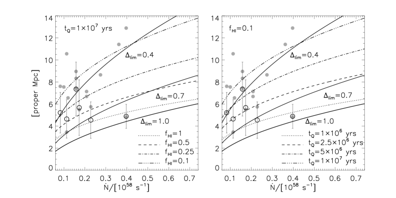
Figure 1: Comparison of the observed sizes of Ly$\alpha$ near-zones as determined by Fan et al. (2006b) (filled grey circles) and Wyithe et al. (2005) (open circles) to the two analytical models discussed in section 2, which predict the extent of the H $\rm\scriptstyle II\$I-front and the size of the Ly$\alpha$ near-zone at $z=6$, respectively. The sizes are plotted as a function of the number of ionizing photons emitted by the quasar per second, $\dot{N}$. The solid curves in both panels give $R_{\alpha}^{\rm max}$ for $\Delta_{\rm lim}=[0.4,0.7,1.0]$. Left: The series of dotted and dashed curves give $R_{\rm ion}$ assuming a uniform IGM with $\Delta=1$, a quasar age of $t_{\rm Q}=10^{7}\rm~{}yrs$ and an IGM neutral hydrogen fraction of $f_{\rm HI}=[1,0.5,0.25,0.1]$. Right: The dotted and dashed curves give $R_{\rm ion}$ assuming a uniform IGM with $\Delta=1$, an IGM neutral hydrogen fraction of $f_{\rm HI}=0.1$ and quasar ages of $t_{\rm Q}=[0.1,0.25,0.5,1]\times 10^{7}\rm~{}yrs$.

Once the near-zone size reaches $R_{\alpha}^{\rm max}$, even if the H $\rm\scriptstyle II\$region around the quasar keeps growing, the residual neutral hydrogen in the ionized region beyond $R_{\alpha}^{\rm max}$ will be sufficient to halt the advance of the observed near-zone edge. Obviously the above definition for the maximum size of the near-zone obviously only makes sense if the amplitude of the metagalactic UV background above the Lyman limit is smaller than $J_{\rm HI}^{\rm lim}$. Also note the size of the observed near-zone in the Ly$\alpha$ region will always be smaller than or equal to $R_{\rm ion}$. The important point to take from this simple argument is the different scaling of the two radii, $R_{\rm ion}\propto\dot{N}^{1/3}$ and $R_{\alpha}^{\rm max}\propto\dot{N}^{1/2}$, with the ionizing luminosity, and that $R_{\alpha}^{\rm max}$ is independent of the neutral hydrogen fraction of the IGM and the lifetime of the quasar. One may also derive a similar expression for the maximum size of the observable Ly$\beta$ near-zone,

$$R_{\beta}^{\rm max}\simeq 2.5\left(\frac{T_{\beta}}{T_{\alpha}}\right)^{0.35}\left(\frac{1+z_{\beta}}{1+z_{\alpha}}\right)^{-9/4}R_{\alpha}^{\rm max},$$ (12)

where $T_{\beta}$ is the IGM temperature at the edge of the Ly$\beta$ near-zone at $z_{\beta}$.

Equations (11) and (12) should be considered as illustrative approximations only; radiative transfer through a realistic IGM density distribution is required to address this fully. A number of caveats should therefore be kept in mind. The upper limits for the near-zone sizes given by equations (11) and (12) do not take into account the possible effect of a damping wing from a significantly neutral IGM, which reduces the size of the Ly$\alpha$ near-zone relative to $\rm Ly\beta$ (Mesinger & Haiman 2004). The presence of the dense, self-shielded clumps responsible for observed Lyman-limit systems will further reduce the upper limit for the observed sizes of the near-zone compared to the estimates given by equations (11) and (12). Additionally, the overlying lower redshift Ly$\alpha$ forest should reduce the observed size of the near-zone in the Ly$\beta$ region. Note that for a predominantly neutral IGM, the sizes of the observed Ly$\alpha$ and Ly$\beta$ near-zones will both trace the position of the H $\rm\scriptstyle II\$I-front and should both be given by $R_{\rm ion}$, whereas if the IGM is highly ionized, the distinction between the near-zone and the general Ly$\alpha$ forest will become highly ambiguous.

However, assuming equation (11) holds, for $R_{\rm ion}>R_{\alpha}^{\rm max}$ ($R_{\rm ion}>R_{\beta}^{\rm max}$) the observed size of the Ly$\alpha$ (Ly$\beta$) near-zone becomes independent of the neutral fraction of the surrounding IGM. The same is true if $R_{\rm ion}=R_{\rm S}$. The timescale for the H $\rm\scriptstyle II\$I-front to reach $R_{\alpha}^{\rm max}$ in a homogeneous IGM is approximately,

$$t\simeq 4.2\times 10^{6}\Delta f_{\rm HI}\left(\frac{R_{\alpha}^{\rm max}}{3.14\rm~{}Mpc}\right)^{3}\left(\frac{\dot{N}}{2\times 10^{57}\rm~{}s^{-1}}\right)^{-1}$$

$$\hskip 8.53581pt\times\left(\frac{1+z}{7}\right)^{3}\rm~{}yrs$$ (13)

For a realistic clumpy IGM in the vicinity of a quasar this timescale should be longer by a factor of a few, but for $f_{\rm HI}<0.1$ this is still considerably shorter than the canonical quasar lifetime of $\sim 10^{7}\rm~{}yrs$ (Martini 2004; Hopkins et al. 2005). The time scale for the H $\rm\scriptstyle II\$I-front to reach $R_{\beta}^{\rm max}$ is $\sim 16$ times longer again. The size of the Ly$\beta$ near-zone is therefore potentially much more sensitive to the IGM neutral hydrogen fraction. A similar argument applies for the scaling of the observed near-zone sizes with quasar age.

2.3 Comparison of the analytical model to observational data

The solid curves in both panels of figure 1 show $R_{\alpha}^{\rm max}$ and its dependence on the number of ionizing photons emitted per second by the quasar, $\dot{N}$, using our fiducial assumptions of $[\tau_{\rm lim},\alpha_{\rm s},T_{\alpha},z_{\alpha}]=[2.3,1.5,2\times 10^{4}\rm~{}K,6]$ in equation (11). The three curves shown are for $\Delta_{\rm lim}=[0.4,0.7,1]$. In the left panel the series of dotted and dashed curves show $R_{\rm ion}$ computed using equation (3) for $f_{\rm HI}=[1,0.5,0.25,0.1]$ and a quasar lifetime of $t_{\rm Q}=10^{7}\rm~{}yrs$. In the right panel $R_{\rm ion}$ is shown for $t_{\rm Q}=[0.1,0.25,0.5,1]\times 10^{7}\rm~{}yrs$ and a fixed neutral fraction of $f_{\rm HI}=0.1$. When computing $R_{\rm ion}$, $\Delta=1$ has been assumed, although in reality $\Delta$ should be slightly larger on average due to the clumpy nature of the IGM. However, we find this does not make any significant difference to our conclusions, as we shall discuss later.

The filled grey circles in figure 1 represent the observed sizes of Ly$\alpha$ near-zones around quasars at $5.81\leq z\leq 6.42$ as determined by Fan et al. (2006b). In the instances where no Mg $\rm\scriptstyle II\$redshift was available, Fan et al. (2006b) have applied a correction to the quasar redshifts of $\Delta z=+0.02$ in order to take into account the systematic redshift offset of high ionization lines. Note further that, as discussed above, Fan et al. (2006b) have smoothed the Ly$\alpha$ spectra to a resolution of $20\rm~{}\AA$ before determining the near-zone sizes. The open circles with error bars are Ly$\alpha$ near-zone sizes as determined by Wyithe et al. (2005) around a sub-sample of the same quasars at $6\leq z\leq 6.42$, adapted from their table 1. Wyithe et al. (2005) used the Ly$\alpha$ near-zone sizes as a proxy for the extent of the quasar H $\rm\scriptstyle II\$I-front, and determine the extent of the near-zones to be at the redshifts where the transmission extending blueward of the Ly$\alpha$ emission line becomes comparable to the noise. The size of Ly$\alpha$ near-zone around $\rm J1030+0524$ they quote was increased to correspond to the size of the slightly larger Ly$\beta$ near-zone observed around this quasar. We have instead adopted $R_{\alpha}=4.55\pm 1.65$, with an error bar based on an uncertainty of $\Delta z=0.03$ in the redshift of $\rm J1030+0524$ (White et al. 2003). We have also omitted $\rm J1048+4637$ from the Wyithe et al. (2005) sample, as this is a BAL quasar which makes a meaningful measurement of the Ly$\alpha$ near-zone size difficult (X.Fan, private communication). For all except one of the quasars ($\rm J1630+4012$, the lowest luminosity quasar) the Wyithe et al. (2005) values are consistent with the corresponding determinations by Fan et al. (2006b) within the error bars shown. As discussed by Fan et al. (2006b) and later within this paper, the observed near-zone sizes evolve rather rapidly with redshift. The larger near-zone sizes within the Fan et al. (2006b) sample which are omitted in the Wyithe et al. (2005) data are for quasars at $z<6$. For both data sets, the conversion from ultraviolet AB absolute magnitudes, $M_{1450}$, to $\dot{N}$ has been made using a generic broken power law spectral energy distribution,

$$L({\nu})\propto\cases{\nu^{-0.5}&($1050<\lambda<1450\,$\AA),\cr\vskip 3.0pt\cr\nu^{-1.5}&($\lambda<1050\,$\AA).\cr}$$ (14)

All photons above $1\rm~{}Ryd$ are considered to be ionizing photons. We have not plotted error bars for $\dot{N}$, although the values will be somewhat uncertain depending on the exact spectrum of the quasars (e.g. Yu & Lu 2005).

As already discussed, the observed size of the near-zone in the Ly$\alpha$ region should be the smaller of $R_{\alpha}^{\rm max}$ or $R_{\rm ion}$. Clearly from figure 1, our simple analytical argument suggests that the sizes of the observed Ly$\alpha$ near-zones are consistent with both the expected extent of classical proximity zones and an H $\rm\scriptstyle II\$I-front expanding into an IGM with a significant neutral hydrogen fraction, for reasonable assumptions for the quasar ionizing luminosity and lifetime. The fact that equation (3) and (11) give similar values for $R_{\rm ion}$ and $R_{\alpha}^{\rm max}$ is a coincidence which explains the discrepant interpretation of the observed sizes of near-zones in the literature. Taking a combination of $0.1\leq f_{\rm HI}\leq 1$ and $10^{6}\leq t_{\rm Q}\leq 10^{7}\rm~{}yrs$ results in an H $\rm\scriptstyle II\$region similar in size to the observed Ly$\alpha$ near-zones, whereas equation (11) reproduces the observed sizes even for small $f_{\rm HI}$ or large $t_{\rm Q}$. For example, one can reasonably adopt values of $f_{\rm HI}=10^{-3}$ and $t=5\times 10^{7}\rm~{}yrs$, within the observationally determined limits of $f_{\rm HI}\geq 10^{-3.5}$ (Fan et al. 2006b) and $10^{6}\leq t_{\rm Q}\leq 10^{8}\rm~{}yrs$ (Martini 2004). For a quasar luminosity of $\dot{N}=2\times 10^{57}\rm~{}s^{-1}$, assuming $\Delta_{\rm lim}=0.4$ and $z_{\alpha}=6$, according to equation (11) one expects to see a Ly$\alpha$ near-zone of $R_{\alpha}\simeq 7.9~{}\rm Mpc$, consistent with observed sizes. However, equation (5) predicts a value of $R_{\rm ion}\simeq 22\rm~{}Mpc$, much larger than any observed Ly$\alpha$ near-zone, although in practise this will be slightly smaller due to the clumpy nature of the IGM. If the size of the observed near-zone is nevertheless identified with $R_{\rm ion}$, the inferred IGM neutral hydrogen fraction is erroneously large.

Therefore, the size of individual near-zones in the Ly$\alpha$ region alone appears to offer little in terms of constraining the ionization state of the hydrogen in the surrounding IGM. This will be confirmed by our detailed numerical simulations including radiative transfer in section 4. However, as we will show, this situation improves if both the Ly$\alpha$ and Ly$\beta$ near-zones are considered in tandem.

3 Creating synthetic absorption spectra including near-zones

3.1 Radiative transfer implementation

Our $1$D radiative transfer implementation is based on an updated version of the multi-frequency photon conserving algorithm used by Bolton et al. (2004). The advantage of this single ray-tracing approach is that we may run many radiative transfer simulations with only modest computational resources. In addition, we achieve the high spatial and temporal resolution which is required to accurately determine post-reionization gas temperatures (Bolton et al. 2004; Tittley & Meiksin 2006). Technical details and the relevant resolution tests can be found in appendices B and C, to which we refer the interested reader.

3.2 Hydrodynamical simulations

We combine our radiative transfer implementation with cosmological density distributions drawn from a large hydrodynamical simulation. The hydrodynamical simulation was run using the parallel TreeSPH code GADGET-2 (Springel 2005). The simulation volume is a periodic box $60h^{-1}$ comoving Mpc in length and contains $2\times 400^{3}$ gas and dark matter particles. Star formation is included using the multi-phase model of Springel & Hernquist (2003) with winds disabled. The simulation was started at $z=99$, with initial conditions generated using the transfer function of Eisenstein & Hu (1999) and cosmological parameters consistent with the combined analysis of three year WMAP and Ly$\alpha$ forest data (Viel et al. 2006; Seljak et al. 2006), $(\Omega_{\rm m},\Omega_{\Lambda},\Omega_{\rm b}h^{2},h,\sigma_{8},n)=(0.26,0.74,0.024,0.72,0.85,0.95)$. The initial gas temperature was set to $T=272.8\rm~{}K$ and the gravitational softening length is $3h^{-1}$ comoving kpc. To check the numerical convergence of our results we also run two further hydrodynamical simulations with lower mass resolution. The different resolution parameters for all three simulations are listed in table LABEL:tab:sims; all other aspects of the lower resolution simulations are identical to the $400^{3}$ run.

Table 1: Hydrodynamical simulation resolution properties. Listed in each column are the total gas particle number, the mass resolution per gas particle and the gravitational softening length.

Gas particle	Gas particle	Softening length
number	mass [$M_{\odot}/h$]	[comoving kpc$/h$]
$120^{3}$	$1.61\times 10^{9}$	$10$
$240^{3}$	$2.01\times 10^{8}$	$5$
$400^{3}$	$4.34\times 10^{7}$	$3$

Table 2: Coordinates and masses of the five most massive haloes in the $400^{3}$ simulation volume at $z=6$. The halo coordinates are given in units of comoving kpc/$h$.

$x_{\rm pos}$	$y_{\rm pos}$	$z_{\rm pos}$	Halo mass [$M_{\odot}$/h]
51030.5	46853.1	18807.6	$2.65\times 10^{12}$
55886.6	49077.1	12091.1	$1.42\times 10^{12}$
52392.1	48011.6	21267.5	$1.33\times 10^{12}$
52061.7	47983.3	22023.3	$1.25\times 10^{12}$
49415.3	47008.2	18859.4	$1.05\times 10^{12}$

A friends-of-friends halo finding algorithm was used to identify the $5$ most massive haloes within the simulation volume in three different snapshots at $z=[6.25,6.0,5.75]$. The total masses (dark matter, gas and stars) and coordinates of the haloes in the $z=6$ snapshot are listed in table LABEL:tab:haloes. These halo masses may be slightly smaller than, or similar to, the expected mass of bright quasar host haloes at $z\simeq 6$. The typical comoving space density of quasars at $z\simeq 6$ is $\sim 10^{-9}\rm~{}Mpc^{-3}$ (Fan et al. 2001), which coincides with the expected abundance of dark matter haloes with mass $\simeq 10^{13}M_{\odot}$ (Mo & White 2002). However, recent observations of molecular gas surrounding $\rm J1148+5251$ indicate its host halo mass may be closer to $\simeq 10^{12}M_{\odot}$ (Walter et al. 2004). Theoretical arguments also suggest that the quasar occupation fraction of massive haloes may be significantly less than unity, perhaps favouring host haloes with lower average masses (Volonteri & Rees 2006). In any case, we have checked that our results depend only weakly on the halo mass by running simulations centred on haloes of smaller mass.

At each redshift, five lines-of-sight where extracted around these haloes, giving $15$ different lines-of-sight in total. To construct the density distributions for the radiative transfer runs we splice together separate lines-of-sight drawn randomly from the simulation volume. The first $30h^{-1}$ comoving Mpc of a spliced line-of-sight is constructed using the density distribution drawn around one of the massive haloes, in which we assume the quasar resides. The remaining $120h^{-1}$ comoving Mpc of the sight-line is made from two further sight-lines drawn randomly from the simulation box at the same redshift. This gives a total length of $150h^{-1}$ comoving Mpc, which is large enough to easily accommodate the observed sizes of Ly$\alpha$ and Ly$\beta$ near-zones at $z\simeq 6$. Each line-of-sight consists of $3000$ pixels with a size of $9.9$ kpc at $z=6$. This provides a good degree of convergence for our radiative transfer simulations (see appendix C for details). For reference, the redshift extent of each line-of-sight at $z=[6.25,6,5.75]$ is $\Delta z=[0.50,0.47,0.45]$. Since the density distributions are drawn from a snapshot at a single redshift, the gas density is rescaled by a factor of $(1+z)^{3}$ along each spliced line-of-sight.

Table 3: Spatially uniform UV background models used for setting the neutral hydrogen and helium fractions of the surrounding IGM. The first two columns list the specific intensity and ionization rate at the Lyman limit in units of $10^{-21}\rm~{}erg~{}s^{-1}~{}cm^{-2}~{}sr^{-1}~{}Hz^{-1}$ and $10^{-12}\rm~{}s^{-1}$ respectively. The last column lists the resulting neutral hydrogen fraction for mean cosmic density at $z=6$ assuming ionization equilibrium at $T=2\times 10^{4}\rm~{}K$. A power law spectrum with $\alpha_{\rm b}=1.5$ has been adopted.

Model	$J_{-21}^{\rm b}$	$\Gamma_{-12}^{\rm b}$	$f_{\rm HI}$
0	0	0	1
1	$2.0\times 10^{-5}$	$5.6\times 10^{-5}$	$3.6\times 10^{-1}$
2	$1.0\times 10^{-4}$	$2.8\times 10^{-4}$	$7.3\times 10^{-2}$
3	$3.0\times 10^{-4}$	$8.5\times 10^{-4}$	$2.4\times 10^{-2}$
4	$1.0\times 10^{-3}$	$2.8\times 10^{-3}$	$7.3\times 10^{-3}$
5	$3.0\times 10^{-3}$	$8.5\times 10^{-3}$	$2.4\times 10^{-3}$
6	$1.0\times 10^{-2}$	$2.8\times 10^{-2}$	$7.3\times 10^{-4}$
7	$3.0\times 10^{-2}$	$8.5\times 10^{-2}$	$2.4\times 10^{-4}$
8	$6.0\times 10^{-2}$	$1.7\times 10^{-1}$	$1.2\times 10^{-5}$
9	$1.0\times 10^{-1}$	$2.8\times 10^{-1}$	$7.3\times 10^{-5}$
10	$2.0\times 10^{-1}$	$5.6\times 10^{-1}$	$3.6\times 10^{-5}$

3.3 Initial conditions

We compute the transfer of radiation through an inhomogeneous hydrogen and helium IGM from a source which emits $\dot{N}$ photons per second above the H $\rm\scriptstyle I\$ionization threshold frequency, where

$$\dot{N}=\int_{\nu_{\rm HI}}^{\infty}L_{\rm HI}\left(\frac{\nu}{\nu_{\rm HI}}\right)^{-\alpha_{\rm s}}d\nu.$$

The source is assumed to have a power law spectrum with index $\alpha_{\rm s}$, typical of quasars, normalised by $L_{\rm HI}$ at the H $\rm\scriptstyle I\$ionization threshold frequency, $\nu_{\rm HI}$. We adopt $\alpha_{\rm s}=1.5$ for this study. The source is placed $10h^{-1}$ comoving kpc from the edge of the line-of-sight; all hydrogen and helium within this radius is assumed to be fully ionized. The distribution of normalised densities $\Delta=\rho_{\rm b}/\bar{\rho}_{\rm b}$ is kept constant during the radiative transfer simulations, while the gas density evolves as $(1+z)^{3}$ as the ionization front progresses along the line-of-sight. This should be a reasonable approximation over a typical quasar lifetime.

We vary the lifetime of the source, $t_{\rm Q}$, the number of ionizing photons emitted per second by the source, $\dot{N}$, and the neutral hydrogen (and helium) fraction of the IGM. To set the neutral fractions in the IGM for each run, we assume the gas is in ionization equilibrium with a spatially uniform UV background. The different UV background models we use are listed in table LABEL:tab:preion, along with the resulting neutral hydrogen fraction at mean density at $z=6$. Note, however, that this does not necessarily correspond to the resulting volume weighted neutral fraction in a simulated sight-line, as on average these will be moderately overdense and have varying gas temperatures, although it gives a rough guide to the expected neutral hydrogen fraction for a given UV background. All UV background models assume a spectral index of $\alpha_{\rm b}=1.5$, although the background spectrum may well be softer if it is dominated by galaxies. This assumption does not have a significant effect on the results of this paper apart from small changes in the neutral helium fraction and the temperature of the IGM. There should also be significant spatial fluctuations in the UV background at $z\simeq 6$ (Wyithe & Loeb 2006; Fan et al. 2006b) but these will only be important at the edge of the quasar near-zone itself and only if the flux from the quasar and the metagalactic ionizing background are similar there. In the latter case spatial fluctuations of the metagalactic ionizing background may affect the measured near-zone sizes.

3.4 Constructing synthetic absorption spectra

We construct synthetic spectra from the output of the radiative transfer simulations as follows. Each line-of-sight is rebinned to have $N=4096$ pixels of proper width $\delta R$, each of which has a neutral hydrogen number density $n_{\rm HI}$, temperature $T$, peculiar velocity $v_{\rm pec}$ and Hubble velocity $v_{\rm H}$ associated with it. The Ly$\alpha$ optical depth in each pixel is computed assuming a Voigt line profile, such that the optical depth in pixel $i$ corresponding to Hubble velocity $v_{\rm H}(i)$ is

$$\tau_{\alpha}(i)=\frac{c\sigma_{\alpha}\delta R}{\pi^{1/2}}\sum_{j=1}^{N}\frac{n_{\rm HI}(j)}{b(j)}H(a,x).$$ (15)

Here $b=(2k_{\rm B}T/m_{\rm H})^{1/2}$ is the Doppler parameter, $\sigma_{\alpha}=4.48\times 10^{-18}\rm~{}cm^{2}$ is the Ly$\alpha$ scattering cross-section and $H(a,x)$ is the Hjerting function (Hjerting 1938)

$$H(a,x)=\frac{a}{\pi}\int^{\infty}_{-\infty}\frac{e^{-y^{2}}}{a^{2}+(x-y)^{2}}~{}dy,$$ (16)

where $x=[v_{\rm H}(i)-u(j)]/b(j)$, $u(j)=v_{\rm H}(j)+v_{\rm pec}(j)$, $a=\Lambda_{\alpha}\lambda_{\alpha}/4\pi b(j)$, $\Lambda_{\alpha}=6.265\times 10^{8}\rm~{}s^{-1}$ is the damping constant and $\lambda_{\alpha}=1215.67\rm~{}\AA$ is the wavelength of the Ly$\alpha$ transition. For Ly$\beta$ optical depths we adopt the same procedure, using instead $\sigma_{\beta}=7.18\times 10^{-19}\rm~{}cm^{2}$, $\Lambda_{\beta}=1.897\times 10^{8}\rm~{}s^{-1}$ and $\lambda_{\beta}=1025.72\rm~{}\AA$. In addition, for the Ly$\beta$ spectra we also add the optical depth contribution from the Ly$\alpha$ forest at lower redshift, $z^{\prime}=[\lambda_{\beta}(1+z)/\lambda_{\alpha}]-1$, where $z$ is the redshift of the Ly$\beta$ pixels. The total Ly$\beta$ optical depth is then $\tau_{\beta}^{\rm tot}(z)=\tau_{\beta}(z)+\tau_{\alpha}(z^{\prime})$. In order to model the Ly$\alpha$ forest at $z^{\prime}$, we use the standard technique of rescaling the optical depth distribution of synthetic spectra, also drawn from our $400^{3}$ simulation at lower redshift, to reproduce the observed mean flux $\langle F\rangle$ of the Ly$\alpha$ forest (see Bolton et al. 2005 for details). The values for the mean flux we adopt in this paper are interpolated from Songaila (2004): $\langle F\rangle=[0.149,0.210,0.223]$ at $z^{\prime}=[5.12,4.91,4.70]$, corresponding to $z=[6.25,6.0,5.75]$.

Figure 2: Examples of the synthetic Ly$\alpha$ and Ly$\beta$ near-zone spectra used in our study. The spectra are drawn from the line-of-sight data shown in figure 4. The quasar is situated on the right of the diagram, and has an age $t_{\rm Q}=10^{7}\rm~{}yrs$ and ionizing luminosity $\dot{N}=2\times 10^{57}\rm~{}s^{-1}$. The surrounding IGM neutral hydrogen fraction is set using UV background model 4, which gives a volume weighted value of $f_{\rm HI}\sim 10^{-2}$. Here the Ly$\alpha$ spectrum has been rebinned to a resolution of $\sim 4\rm~{}\AA$ per pixel and Gaussian distributed noise with a total signal to noise of $20$ per pixel has been added, typical of moderate resolution quasar spectra. The Ly$\beta$ spectrum has been rebinned to have the same bin size as the Ly$\alpha$ spectrum in velocity space. The solid line in each panel marks the extent of the quasar H $\rm\scriptstyle II\$region, some way ahead of the edge of spectroscopically identified Ly$\alpha$ and Ly$\beta$ near-zones. These both lie at a distance of $\sim 8.3$ proper Mpc from the quasar. The dotted line shows the adopted flux threshold, $F_{\rm lim}=0.1$, used to identify the edge of the near-zone.

Figure 3: Left: Density distributions at $z=6$ drawn from hydrodynamical simulations with differing mass resolution. The dotted, dashed and solid lines correspond the $120^{3}$, $240^{3}$ and $400^{3}$ simulations respectively. The corresponding mass resolutions are listed in table LABEL:tab:sims. Centre: The neutral hydrogen number density normalised by the total hydrogen number density as predicted by the radiative transfer algorithm for a quasar within the massive halo situated on the right hand side of the density distribution. Right: The resulting Ly$\alpha$ near-zone profile.

For comparison to observational data, we must also mimic the typical resolution and noise of quasar spectra at $z\simeq 6$. The values for these vary in the literature from one line-of-sight to the next. We adopt a spectral resolution of $4\rm~{}\AA$ per pixel by rebinning our simulated spectra and adding Gaussian distributed noise with a total signal-to-noise ratio of $20$ per pixel at the continuum level (e.g. Fan et al. 2000) and a constant read-out signal-to-noise of $80$ per pixel. Example synthetic Ly$\alpha$ and Ly$\beta$ spectra are shown in figure 2.

3.5 Hydrodynamical simulation resolution

To simulate the propagation of ionizing radiation through an inhomogeneous IGM, the structure of the IGM must be sufficiently resolved to correctly model the number of ionizing photon absorption events per unit volume (e.g. Kohler et al. 2005; Iliev et al. 2006b; Gnedin & Fan 2006). We test this using the hydrodynamical simulations listed in table LABEL:tab:sims. We firstly select one of our spliced lines-of-sight at $z=6$ from the $400^{3}$ simulation, and construct lines-of-sight from the same location in the lower resolution simulations. For all three lines-of-sight we then use the radiative transfer code to model the propagation of ionizing radiation from a quasar with $\dot{N}=5\times 10^{57}\rm~{}s^{-1}$ and $t_{\rm Q}=10^{7}\rm~{}yrs$ into fully neutral hydrogen and helium gas. We subsequently extract the Ly$\alpha$ absorption spectra.

The results of this test are shown in figure 3. From left to right the panels show the density distribution, neutral hydrogen fraction and the resulting Ly$\alpha$ near-zone profile drawn from the radiative transfer runs in all three sight-lines. The degree of convergence in the H $\rm\scriptstyle II\$I-front position is good. The highest resolution simulation resolves a greater number of overdense peaks, but the effect that this has on the I-front position is counteracted by better resolved voids. The main difference is that one sees more detailed structure in the higher resolution simulation spectra. Note also the smooth nature of the Ly$\alpha$ near-zone profile due to the damping wing from the neutral IGM; the edge of the Ly$\alpha$ near-zone lies behind the H $\rm\scriptstyle II\$I-front as a result (e.g. Mesinger & Haiman 2004). We conclude that the $400^{3}$ hydrodynamical simulation is sufficiently resolved for the purpose of this work with one caveat; the very dense regions responsible for Lyman limit absorption systems will not be sufficiently resolved. We will come back to this in section 5.

4 Multi-frequency radiative transfer through cosmological density fields

4.1 An example line-of-sight

Figure 4: An example line-of-sight used in our analysis of near-zone sizes. The top panel shows the normalised density distribution along the line-of-sight drawn from a large hydrodynamical simulation at $z=6$ against distance from the quasar; the quasar host halo is on the right hand side of the diagram. Subsequent panels show the output from the radiative transfer algorithm for a quasar of age $t_{\rm Q}=10^{7}\rm~{}yrs$ and ionizing luminosity $\dot{N}=2\times 10^{57}\rm~{}s^{-1}$. UV background model $4$ was used, producing an IGM with a volume weighted neutral hydrogen fraction $f_{\rm HI}\sim 10^{-2}$. In descending order the panels display the H $\rm\scriptstyle I$, He $\rm\scriptstyle II\$and He $\rm\scriptstyle III\$number densities normalised by the total hydrogen number density, the gas temperature, the peculiar velocity (drawn from the hydrodynamical simulation), the H $\rm\scriptstyle I$, He $\rm\scriptstyle I\$and He $\rm\scriptstyle II\$ionization rates and the energy input per ionization for H $\rm\scriptstyle I$, He $\rm\scriptstyle I\$and He $\rm\scriptstyle II$. The last panel shows the resulting Ly$\alpha$ spectrum with a resolution and signal-to-noise resembling observed high quality, high resolution quasar spectra.

In figure 2 we had shown synthetic absorption spectra for an example line-of-sight at $z=6$. Figure 4 shows a variety of physical properties along the same line-of-sight together with a high resolution, high signal-to-noise version of the Ly$\alpha$ region of the absorption spectrum. The quasar is on the the right hand side of the plot. The scale on the horizontal axis corresponds to the distance from the quasar in proper Mpc. The top panel shows the normalised density $\Delta$ along the line-of-sight. In the subsequent panels the output from the radiative transfer code is shown. In descending order the panels display the H $\rm\scriptstyle I$, He $\rm\scriptstyle II\$and He $\rm\scriptstyle III\$number densities normalised by the total hydrogen number density, the gas temperature, the peculiar velocity (drawn from the hydrodynamical simulation), the H $\rm\scriptstyle I$, He $\rm\scriptstyle I\$and He $\rm\scriptstyle II\$ionization rates and the energy input per ionization for H $\rm\scriptstyle I$, He $\rm\scriptstyle I\$and He $\rm\scriptstyle II$. The last panel shows the resulting Ly$\alpha$ near-zone spectrum. The ionizing source has an age $t_{\rm Q}=10^{7}\rm~{}yrs$, luminosity $\dot{N}=2\times 10^{57}\rm~{}s^{-1}$ and UV background model $4$ has been adopted.

There are a few interesting points to note about figure 4 before proceeding. Firstly, the H $\rm\scriptstyle II\$I-front has reached $\sim 11.8\rm~{}Mpc$, which is somewhat smaller than the value of $R_{\rm ion}=16.6\rm~{}Mpc$ one predicts with equation (3) assuming $\Delta=1$. This difference is largely due to the clumpy nature of the IGM and to a lesser extent the presence of helium. Adopting $\Delta=2.2$, the actual mean normalised density along the line-of-sight, equation (3) predicts $R_{\rm ion}=11.8\rm~{}Mpc$, consistent with the simulation results. It is the mean density of the gas which limits the propagation of the I-front in this instance. In comparison, the He $\rm\scriptstyle III\$I-front has reached the significantly smaller distance of $\sim 4.1$ Mpc from the source. The large difference in the extent of the He $\rm\scriptstyle III\$and H $\rm\scriptstyle II\$I-fronts is due to the smaller fraction of H $\rm\scriptstyle I\$compared to He $\rm\scriptstyle II\$for the assumed metagalactic UV background.

The amount by which the quasar He $\rm\scriptstyle III\$I-front lags behind the H $\rm\scriptstyle II\$I-front depends sensitively on the H $\rm\scriptstyle I\$to He $\rm\scriptstyle II\$ratio in the surrounding IGM. Note that for a fully neutral IGM the extent of He $\rm\scriptstyle III\$and H $\rm\scriptstyle II\$I-fronts should be very similar for typical quasar spectral index (Madau et al. 1999). There is also evidence for a clear break in the mean temperature of the IGM around $4\rm~{}Mpc$, corresponding to the He $\rm\scriptstyle III\$I-front position. The higher temperature is due to radiative transfer effects boosting the average energy per ionization when the He $\rm\scriptstyle II\$is reionized by the quasar (Abel & Haehnelt 1999; Bolton et al. 2004). This effect becomes progressively larger for higher neutral helium fractions. Hence the widths of Ly$\alpha$ absorption features observed in high resolution spectra of quasar near-zones (e.g. Becker et al. 2005) and their correlation (or lack of) with distance from the quasar, combined with a lower limit to the extent of the H $\rm\scriptstyle II\$I-front, contain interesting information on the ionization state of hydrogen and helium in the IGM as well as the spectral index of the source. However, this may be complicated by the presence of high temperature shocked gas near the quasar host halo. Detailed modelling will be needed before any firm conclusions can be drawn from observational data.

The second and third last panels in figure 4 show the behaviour of the combined quasar and metagalactic background radiation fields at three frequencies, corresponding to the ionization thresholds of H $\rm\scriptstyle I$, He $\rm\scriptstyle I\$and He $\rm\scriptstyle II$. The quasar radiation field falls in intensity due to increasing distance from the quasar and the decreasing photon mean free path, until the ionization rate per atom/ion drops to the uniform value adopted for the UV background model. The filtering effect of radiative transfer on the spectrum of the quasar radiation field is clearly visible in the second last panel. Higher energy photons have a longer mean free path, boosting the average energy per ionization in places where the gas is optically thick and the spectrum has consequently hardened. Note that the energy per ionization for H $\rm\scriptstyle I\$actually decreases somewhat between the H $\rm\scriptstyle II\$and He $\rm\scriptstyle III\$I-fronts because the photo-heating rate for H $\rm\scriptstyle I\$falls in this region as high energy photons are soaked up by the optically thick helium.

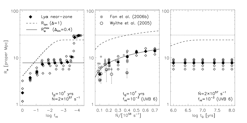
Figure 5: The sizes of Ly$\alpha$ near-zones around quasars at $z=6$ computed from radiative transfer simulations in an inhomogeneous hydrogen and helium IGM. In the left panel the IGM neutral hydrogen fraction is varied for a fixed quasar age and luminosity, in the central panel the quasar luminosity is varied for fixed quasar age and IGM neutral hydrogen fraction, and in the right panel the quasar age is varied for fixed quasar luminosity and IGM neutral hydrogen fraction. The values of the fixed quantities are listed in the bottom right of each panel. The sizes of Ly$\alpha$ near-zones for individual lines-of-sight are shown with the open diamonds, with the average for each parameter set shown by the filled diamonds. The solid curves correspond to $R_{\alpha}^{\rm max}$ for $\Delta_{\rm lim}=0.4$, the dashed curves correspond to $R_{\rm ion}$ for $\Delta=1$ and the dotted line indicates the length of the simulated sight-line. The filled grey circles and open circles in the central panel show the observed sizes of Ly$\alpha$ near-zones, as determined by Fan et al. (2006b) and Wyithe et al. (2005) respectively.

Finally, the bottom panel in figure 4 shows the resulting Ly$\alpha$ spectrum for a pixel size of $\sim 0.25\rm~{}\AA$. A signal-to-noise per pixel of $20$ at the continuum level has been adopted, with a constant read-out signal-to-noise of $100$ per pixel. Spectra of similar quality are already obtainable with current instruments (Becker et al. 2005; Becker et al. 2006b). However, for the synthetic spectra used in this paper we adopt the moderate spectral resolution shown in figure 2, which is more typical of most of the observational data. The solid vertical lines in both panels in figure 2 mark the extent of the quasar H $\rm\scriptstyle II\$region at $11.8$ Mpc. Clearly the extent of the Ly$\alpha$ near-zone, $R_{\alpha}\simeq 8.3$ Mpc, is some way behind the H $\rm\scriptstyle II\$I-front. Note also that the extent of the Ly$\beta$ and Ly$\alpha$ near-zones are the same even though the volume weighted neutral fraction of the IGM in this line-of-sight is $\sim 10^{-2}$ prior to the quasar switching on. In this instance, naively using equation (12), one might expect the Ly$\beta$ near-zone to be somewhat larger than the Ly$\alpha$ near-zone. The reason for the similarity in their size is clear on examining the density distribution along this particular sight line, shown in the top panel in figure 4. The transmission peaks in the Ly$\alpha$ and Ly$\beta$ spectra at $\sim 8.3$ Mpc correspond to the very low density void at the same position in the density distribution. Beyond this there are several high density clumps which attenuate the quasar radiation field and prevent any further transmission in either spectra. Consequently, variations in the density distribution of the IGM, as well as the potential insensitivity of the Ly$\alpha$ near-zone size to the neutral hydrogen fraction, will make attempts to determine $f_{\rm HI}$ using near-zone sizes difficult. Combining the Ly$\alpha$ and Ly$\beta$ near-zone sizes obviously helps, but this will not necessarily give the correct extent of the quasar H $\rm\scriptstyle II\$region for any individual spectrum either. As we will discuss in more detail later, reasonably large samples of high quality data will be required to better determine the ionization state of the surrounding IGM using near-zone sizes. We further note that the presence of the lower redshift Ly$\alpha$ forest in the Ly$\beta$ spectrum clearly reduces the amplitude of the Ly$\beta$ transition and in some cases will block transmission peaks from the Ly$\beta$ near-zone.

4.2 The measured sizes of Ly$\alpha$ near-zones in cosmological density fields

In figure 5 we explore the dependence of Ly$\alpha$ near-zone sizes on the ionization state of the surrounding IGM and the luminosity and lifetime of quasars using realistic density distributions drawn from our cosmological hydrodynamical simulation. The left panel shows the dependence of Ly$\alpha$ near-zone sizes on the volume weighted IGM neutral hydrogen fraction. For each neutral hydrogen fraction we have performed a full radiative transfer calculation for the five different lines-of-sight drawn from our simulation box at $z=6$. The near-zone sizes were measured out to our fiducial flux limit of $F_{\rm lim}=e^{-2.3}=0.1$, and are shown by the open diamonds in figure 5. Note that some of these data points fall on top of each other, giving the appearance of less than five data points for some of the parameters. The resolution of each synthetic spectrum was degraded and noise was added to mimic the observational data. The larger filled diamonds show the average value of $R_{\alpha}$ for each parameter set. The neutral hydrogen fraction of the surrounding IGM was varied using UV background models $0-10$, described in table LABEL:tab:preion. The lifetime and luminosity of the quasar were fixed at $t_{\rm Q}=10^{7}\rm~{}yrs$ and $\dot{N}=2\times 10^{57}\rm~{}s^{-1}$, respectively. The solid curve shows $R_{\alpha}^{\rm max}$ assuming $\Delta_{\rm lim}=0.4$. The dashed curve shows $R_{\rm ion}$ assuming $\Delta=1$ and the horizontal dotted line corresponds to the length of each simulated line-of-sight.

The first point to note about figure 5 is the considerable spread in the inferred near-zone sizes from one line-of-sight to the next when all other parameters are fixed. This highlights the importance of taking into account the effect of a realistic density field containing voids and overdense clumps on the observed size and appearance of the near-zone. In particular, as in figure 2, it is the most underdense voids within the quasar H $\rm\scriptstyle II\$region which set the observed extent of the spectroscopically identified Ly$\alpha$ near-zone.

We can now investigate how the actual near-zone sizes relate to our analytical estimates for $R_{\rm ion}$ and $R_{\alpha}^{\rm max}$ given in section 2. Firstly, we consider the effect of varying the surrounding IGM neutral hydrogen fraction, as shown in the left hand panel of figure 5. For large values of the neutral hydrogen fraction the observed Ly$\alpha$ near-zone size can be approximated by $R_{\rm ion}$, albeit with an offset from our chosen value of $\Delta=1$ due to gas clumping. The near-zone size increases with decreasing neutral fraction as $f_{\rm HI}^{-1/3}$, but note also the slight deviation of the data point for an entirely neutral IGM from the expected scaling due to the presence of an extended damping wing from the Gunn-Peterson trough. As expected the observed sizes saturate at $R_{\alpha}^{\rm max}$ where they do not increase further with decreasing neutral fraction until $f_{\rm HI}\leq 10^{-3.5}$. However, even for $f_{\rm HI}>0.1$ it is difficult to determine the neutral fraction accurately from a small sample of absorption spectra due to the rather large scatter in near-zone sizes. Evaluating equation (13) using $R_{\alpha}^{\rm max}=7.85$, corresponding to $\Delta_{\rm lim}=0.4$ in equation (11), and $f_{\rm HI}\geq 0.1$ results in a timescale for the H $\rm\scriptstyle II\$I-front to reach $R_{\alpha}$ greater than or similar to the assumed quasar age of $t_{\rm Q}=10^{7}\rm~{}yrs$ if $\Delta\geq 1$. For the chosen values of the quasar ionizing luminosity and lifetime, saturation thus occurs at $f_{\rm HI}<0.1$. For larger quasar ionizing luminosity or longer lifetime the saturation would occur at larger neutral fraction and vice versa.

For neutral hydrogen fractions smaller than $10^{-3.5}$, the Ly$\alpha$ near-zone sizes measured using our definition (see section 2.2) increase rapidly as transmission from the IGM ionized by the metagalactic UV background rather than the quasar becomes more common. Strictly speaking, these sizes no longer correspond to the regions impacted by the quasar ionizing radiation. With further decreasing neutral fraction the near zone sizes rapidly approach the box-size of the numerical simulation shown by the dotted line. This is one of the reasons why Fan et al. (2006b) take the necessary step of smoothing their Ly$\alpha$ spectra to obtain the Ly$\alpha$ near-zone sizes; not doing so makes distinguishing between the many thin transmission peaks from the highly ionized, underdense IGM and the true edge of the near-zone very difficult. However, smoothing will have the effect of attributing transmission peaks from the IGM to the size of the quasar near-zone, influencing the perceived evolution in smoothed near-zone sizes in the regime where the IGM makes the transition from being optically thick to optically thin. One must be aware of this effect when interpreting data which has been smoothed. We discuss this in further detail in section 5.

In the middle and right panels of figure 5 we show the dependence of the Ly$\alpha$ near-zone size on quasar ionizing luminosity and quasar lifetime for an IGM neutral hydrogen fraction $f_{\rm HI}\simeq 10^{-3}$ (UV background model $6$). The dashed and solid curves again show $R_{\rm ion}$ and $R_{\alpha}^{\rm max}$, respectively. The simulated near-zone sizes scale with ionizing luminosity as $R_{\alpha}\propto\dot{N}^{1/2}$ and are independent of the lifetime of the quasar as expected for this neutral hydrogen fraction, where $R_{\alpha}=R_{\alpha}^{\rm max}$. Note that for a significantly neutral IGM with $f_{\rm HI}\geq 0.1$, one would see an evolution in the near-zone size roughly proportional to $t_{\rm Q}^{1/3}$ until $t_{\rm Q}\geq 10^{7}\rm~{}yrs$. Overall, the analytic approximations $R_{\rm ion}$ and $R_{\alpha}^{\rm max}$ appear to provide a reasonable guide for understanding the nature of quasar near-zones for $10^{-3}\leq f_{\rm HI}\leq 1$.

The filled grey circles and open circles in the middle panel show the observed sizes of Ly$\alpha$ near-zones as determined by Fan et al. (2006b) and Wyithe et al. (2005) respectively. There is good agreement between the smaller near-zone sizes and the model, suggesting consistency with $f_{\rm HI}\sim 10^{-3}$ in these cases. The larger near-zone sizes, predominantly at $z<6$, lie somewhat above the values from the simulated spectra, but the uncertainties in the source luminosity, the measured near-zone size and the near-zone size distribution due to cosmic variance should be kept in mind. We will come back to this point later. Note also again that the simulated spectra discussed here have not been smoothed. As we will see in section 5, if we smooth the spectra this discrepancy becomes larger.

4.3 Comparing Ly$\alpha$ and Ly$\beta$ near-zone sizes

In the last section we demonstrated that $R_{\alpha}$ alone is not very sensitive to the ionization state of the surrounding IGM for typical quasar ionizing luminosities and lifetimes. This is due to the saturation of the near-zone size for a low neutral hydrogen fractions at $R_{\alpha}^{\rm max}$ and the large scatter in near-zone sizes due to density fluctuations. The relative size of $R_{\alpha}$ and $R_{\beta}$ is an independent probe of the ionization state which stays useful when $R_{\alpha}$ is saturated at $R_{\alpha}^{\rm max}$. In figure 6 we compare the Ly$\alpha$ and Ly$\beta$ near-zone sizes predicted by $20$ of the radiative transfer simulations with progressively smaller IGM neutral hydrogen fractions. The solid line shows $R_{\beta}=2.5R_{\alpha}$, which is the approximate upper limit to the expected size of the Ly$\beta$ near-zone predicted by equation (12). The dotted line shows $R_{\alpha}=R_{\beta}$, the expected relation when the IGM is substantially neutral. As noted earlier, these theoretical limits ignore the effect of foreground absorption from the lower redshift Ly$\alpha$ forest on observed Ly$\beta$ near-zone sizes. However, we do include this effect in the synthetic spectra analysed here.

For $f_{\rm HI}\geq 10^{-2}$ the simulated spectra appear to follow the $R_{\beta}=R_{\alpha}$ relation. For small neutral hydrogen fractions ($f_{\rm HI}\sim 10^{-3}$) the data exhibit an upward deviation approaching but not reaching the $R_{\beta}=2.5R_{\alpha}$ relation. This suggests that the inhomogeneous IGM, and to a lesser extent the additional absorption from the Ly$\alpha$ forest in the Ly$\beta$ spectrum, combined with limited spectral resolution, reduces the Ly$\beta$ near-zone sizes more strongly than the Ly$\alpha$ near-zone sizes. Hence, for $f_{\rm HI}\sim 10^{-2}$ (UV background model 4) the Ly$\alpha$ and Ly$\beta$ near-zone sizes can still be rather similar.

Note that for some of the completely neutral IGM models (UV background model 0), $R_{\beta}$ is slightly larger than $R_{\alpha}$ due to the Ly$\alpha$ Gunn-Peterson trough damping wing (e.g. Mesinger & Haiman 2004). In the absence of this effect one would expect $R_{\alpha}\simeq R_{\beta}$, since $R_{\alpha}$ has still not reached its maximum and thus both near-zones trace the extent of the H $\rm\scriptstyle II\$I-front. Note further that the time scale for the H $\rm\scriptstyle II\$I-front to reach $R_{\beta}$ is around $16$ times longer than the timescale to reach $R_{\alpha}$. Consequently, the Ly$\beta$ near-zone keeps increasing in size for some time after the Ly$\alpha$ near-zone has ceased to expand. This can be seen by comparing the results for UV background models 4 and 6.

Figure 6: The ratio of Ly$\alpha$ to Ly$\beta$ near-zone sizes for inhomogeneous IGM models with differing volume weighted neutral hydrogen fractions. An ionizing photon production rate of $\dot{N}=2\times 10^{57}\rm~{}s^{-1}$ and age of $t_{\rm Q}=10^{7}\rm~{}yrs$ has been assumed for the quasar. The solid line shows $R_{\beta}=2.5R_{\alpha}$, which is the approximate upper limit to the size of the Ly$\beta$ near-zone predicted by equation (12), while the dotted line shows $R_{\alpha}=R_{\beta}$. The filled circle with error bars show the observationally determined sizes of the Ly$\alpha$ and Ly$\beta$ near-zones around $\rm J1030+0524$ (White et al. 2003).

The filled circle with error bars show the observationally determined size of the Ly$\alpha$ and Ly$\beta$ near-zones around $\rm J1030+0524$ taken from White et al. (2003). We have assumed an uncertainty in the quasar redshift of $\Delta z=0.03$. Its location close to the $R_{\alpha}=R_{\beta}$ line appears to suggest that $f_{\rm HI}\geq 10^{-2}$. However, the large scatter in near-zone size makes it very difficult to come to definite conclusions for individual systems.

5 The observed redshift evolution of near-zone sizes

5.1 The simulations

In a recent paper Fan et al. (2006b) (hereinafter F06b) present evidence for evolution in the size of Ly$\alpha$ near-zone sizes with redshift. The conclusion of F06b using a sample of $16$ quasars, was that the average Ly$\alpha$ near-zone size increases by a factor of $2.8$ from $z=6.4$ to $z=5.7$ after correcting for quasar luminosity differences. Assuming that $R_{\alpha}\propto(1+z)^{-1}f_{\rm HI}^{-1/3}$, F06b note this corresponds to $f_{\rm HI}$ decreasing by a factor of $\sim 14$. Assuming a value of $f_{\rm HI}\sim 9.3\times 10^{-5}$ at $z=5.7$ based on their direct optical depth measurements suggests $f_{\rm HI}\sim 1.3\times 10^{-3}$ at $z=6.4$. However, as we have shown already, the dependence of the Ly$\alpha$ near-zone size on $f_{\rm HI}$ is not so straightforward. We shall attempt to model this evolution here using three different scenarios for the IGM neutral hydrogen fraction evolution within our radiative transfer implementation.

In all three scenarios, we shall consider a quasar embedded in an inhomogeneous hydrogen and helium IGM. We set the quasar to have the fiducial values $\dot{N}=2\times 10^{57}\rm~{}s^{-1}$ and $t_{\rm Q}=10^{7}\rm~{}yrs$. As before, the IGM density distributions used for the radiative transfer runs are drawn in different directions around the $5$ most massive haloes in the simulation volume at $z=[6.25,6,5.75]$, giving a total of $15$ different lines-of-sight for comparison to the F06b data. In the first scenario we simulate the propagation of radiation from the source into the IGM at $z=[6.25,6,5.75]$ using UV background models 6, 9 and 10 respectively. These UV background models reproduce volume weighted neutral hydrogen fractions which are consistent with estimates from the direct Gunn-Peterson optical depth measurements of F06b. This scenario corresponds to a moderate evolution of the IGM neutral fraction with redshift. In the second scenario we use UV background models 1, 6 and 10 at $z=[6.25,6,5.75]$, respectively. This scenario corresponds to a rapid evolution in the IGM neutral hydrogen fraction above $z=6$, where UV background model 1 corresponds to a substantially neutral IGM at $z=6.25$, consistent with the lower limits on $f_{\rm HI}$ from both Mesinger & Haiman (2004) and Wyithe et al. (2005). In the third scenario, we also adopt a moderate evolution in the neutral hydrogen fraction, but in addition take into account the effect of self-shielded dense clumps. These systems are expected to be responsible for Lyman limit systems, but our hydrodynamical simulations do not fully resolve them. To include them we use a simple model for self-shielded clumps based on the model of reionization in the post-overlap phase by Miralda-Escudé et al. (2000). The details of this model are described in appendix D.

5.2 The relative sizes of Ly$\alpha$ near-zones and their evolution with redshift

Figure 7: The evolution of Ly$\alpha$ and Ly$\beta$ near-zone size with redshift for different IGM neutral hydrogen fractions. Each panel shows the composite absorption profile constructed from $5$ lines-of-sight in redshift bins at $z=[6.25,6,5.75]$. The spectra have been degraded to resemble observational spectra and then smoothed to a resolution of $20\rm~{}\AA$. The Ly$\alpha$ profiles are shown on the left hand side, with the Ly$\beta$ profiles on the right. In all cases the quasar has an age of $t_{\rm Q}=10^{7}\rm~{}yrs$ and an ionizing photon production rate of $\dot{N}=2\times 10^{57}\rm~{}s^{-1}$. Top: Near-zone sizes for an IGM ionized by a uniform metagalactic UV background, corresponding to the moderate evolution scenario. Centre: The UV background models are now chosen to produce a rapid evolution in the neutral hydrogen fraction. Bottom: Near-zone sizes for an IGM which is highly ionized at low densities by a uniform UV background but is completely neutral above a fixed density threshold. This mimics the behaviour of dense self-shielded clumps responsible for Lyman limit systems.

As discussed in previous sections and by F06b, determining the absolute sizes of the near-zones is plagued with a range of uncertainties. One should, however, hope that these uncertainties depend weakly on redshift. Therefore, in this section we will firstly investigate the redshift evolution in the relative sizes of Ly$\alpha$ near-zones found by F06b. We undertake a comparison of the absolute near-zone sizes with the observations of F06b in the next section. The evolution of the synthetic Ly$\alpha$ and Ly$\beta$ near-zone sizes with redshift for our three scenarios is shown in figure 7, similar to figure 13 in F06b. We note however that figure 13 in F06b is not corrected for the quasar luminosity, whereas for the simulations used in figure 7 we have assumed a constant value of $\dot{N}=2\times 10^{57}\rm~{}s^{-1}$. In addition, the spectra in each bin in figure 13 of F06b are from a range of redshifts, rather than all at the same redshift.

Following F06b, the simulated spectra are smoothed to a resolution of $20\rm~{}\AA$ and the composite absorption profile of the $5$ lines-of-sight at each redshift is plotted. To compare these data to the observational results of F06b, we adopt their definition of the Ly$\alpha$ near-zone. This is defined as the extent of the smoothed spectrum where the normalised flux is greater than $0.1$. This hopefully provides a more robust way of defining $R_{\alpha}$ when we are considering examples where transmission from the thinning Ly$\alpha$ forest affect the extent of the near-zones.

The data in the top panels in figure 7 correspond to the moderate evolution scenario. Between $z=5.75$ and $z=6.25$, the Ly$\alpha$ near-zone size decreases by a factor of $2.1$. This is slightly less than the amount of evolution seen by F06b from $z=5.7$ to $z=6.4$, but is consistent with the their data over the smaller redshift range we consider. Using the theoretical scaling $R_{\alpha}\propto(1+z)^{-1}f_{\rm HI}^{-1/3}$, this would imply that the IGM neutral hydrogen fraction has changed by a factor $\sim 7$ over the range $5.75\leq z\leq 6.25$. However, the average volume weighted IGM neutral hydrogen fraction used in each redshift bin in the top panels is $f_{\rm HI}=[1.6\times 10^{-3},1.5\times 10^{-4},8.1\times 10^{-5}]$ at $z=[6.25,6,5.75]$. Thus, the IGM neutral fraction we use actually changes by a factor of $\sim 20$ over this range. Note that there is little evolution in the composite Ly$\alpha$ near-zone sizes between $z=6.25$ and $z=6$ because the sizes of the near-zones are just leaving the saturated regime. A substantial part of the evolution of the near-zone size therefore occurred for the rather small change in neutral fraction between $z=5.75$ and $z=6$, where the IGM neutral hydrogen fraction changes by less than a factor of two. In this redshift range the Ly$\alpha$ near-zones sizes are no longer near the saturated regime, which occurs approximately for $10^{-3}\leq f_{\rm HI}\leq 10^{-1}$. In this instance, transmission from the IGM ionized by the UV background contributes to the Ly$\alpha$ near-zone size in the smoothed spectra; the flux from the quasar at the edge of the near-zone is comparable to the flux of the metagalactic UV background ionizing the surrounding IGM. Therefore, relatively small changes in the highly ionized IGM neutral hydrogen fraction can produce a rapid evolution in the observed sizes of Ly$\alpha$ near-zones using the F06b definition of near-zone sizes. This occurs at a neutral hydrogen fraction of $f_{\rm HI}\sim 10^{-4}$. Rapid evolution in the smoothed Ly$\alpha$ near-zone sizes over the redshift range $5.75\leq z\leq 6.25$ is therefore not necessarily strong evidence for a significantly neutral IGM just above $z=6$. We briefly note that we have tested this further by varying the flux limit used to define the smoothed near-zone sizes. For $F_{\rm lim}>0.1$, the redshift evolution in the smoothed near-zone sizes is somewhat weaker. It should be an interesting test to perform the same exercise on the observed data.

In the top right panel we show the corresponding composite absorption profiles for the Ly$\beta$ near-zones. The level of transmission in the Ly$\beta$ near-zone is $2-3$ times lower compared to the Ly$\alpha$ near-zone. This is mainly due to foreground Ly$\alpha$ absorption from gas at lower redshift. The F06b definition for $R_{\alpha}$ is therefore not appropriate as a definition for $R_{\beta}$. The transmission profile of the Ly$\beta$ near-zone is much shallower, more extended and fluctuates strongly. The Ly$\beta$ near-zones all extend beyond the extent of the corresponding Ly$\alpha$ near-zones, albeit by only around one Mpc at $z=6.25$. This is expected since the optical depth for Ly$\beta$ absorption is smaller and larger neutral hydrogen fractions can be probed.

In the central panels we show the results for the rapid evolution scenario, with $f_{\rm HI}=[3.1\times 10^{-1},1.4\times 10^{-3},8.1\times 10^{-5}]$ at $z=[6.25,6,5.75]$. In this case, the composite Ly$\alpha$ near-zone size decreases by factor of $3.1$ from $z=5.75$ to $6.25$. This is somewhat larger than the F06b observed evolution. Again the scaling $R_{\alpha}\propto(1+z)^{-1}f_{\rm HI}^{-1/3}$ would imply that $f_{\rm HI}$ has changed by a factor of $24$, compared to an actual change by a factor of over $3800$. However, most of the near-zone size evolution in the centre-left panel has again occurred for the rather small change in neutral fraction between $z=5.75$ and $z=6$. In the centre-right panel, at $z=6$ the Ly$\beta$ transmission extends beyond the Ly$\alpha$ transmission as before. In the $z=6.25$ case the Ly$\beta$ transmission extends the same distance as the Ly$\alpha$ transmission, since in this case the edge of the near-zones correspond to the quasar H $\rm\scriptstyle II\$I-front. As discussed earlier, the Ly$\alpha$ and Ly$\beta$ near-zones are expected to have a similar size for an IGM with $f_{\rm HI}\geq 10^{-2}$ within our models. A comparison of the Ly$\alpha$ and Ly$\beta$ near-zones sizes for a large sample of high quality quasar spectra should thus tell whether the IGM is significantly neutral just above $z=6$ or not.

Finally, in the bottom panels we show the mean absorption profiles for models which also take into account the effect of self-shielded clumps (SSCs), as described in appendix D. These models should be a more realistic representation of the post-overlap phase of reionization (Miralda-Escudé et al. 2000; Gnedin 2000). The average volume weighted neutral hydrogen fraction in each redshift bin for these models is $f_{\rm HI}=[7.4\times 10^{-2},1.1\times 10^{-2},4.3\times 10^{-3}]$ at $z=[6.25,6,5.75]$. Note, however, that the volume weighted neutral fractions are considerably lower if the SSCs are excluded, i.e. for the IGM with $\Delta<\Delta_{\rm SSC}$. Excluding regions with $\Delta\geq\Delta_{\rm SSC}$ the neutral hydrogen fractions in the highly ionized IGM are $f_{\rm HI}(\Delta<\Delta_{\rm SSC})=[7.9\times 10^{-4},7.3\times 10^{-5},3.5\times 10^{-5}]$. These values are similar to those used for the moderate evolution scenario in the top panels. Compared to the models with no SSCs in the top panels, there is little difference in the Ly$\alpha$ and Ly$\beta$ near-zones shown in the bottom panels. Note that although the volume weighted neutral hydrogen fraction is high in these sight-lines, especially at $z=6.25$, the low density regions which dominate the transmission features are still highly ionized. Therefore, the inclusion of SSCs appears to have little effect on the propagation of the quasar I-front. This is perhaps not too surprising as the SSCs would have to contain a significant fraction of the total hydrogen mass in neutral form in order induce a significant evolution in the near-zone sizes with redshift. For a highly ionized IGM the SSCs are therefore not important. This may, however, be different for smaller neutral fractions and/or at higher redshift.

In summary, the relative sizes of Ly$\alpha$ near-zones and their evolution with redshift are consistent with a moderate change in the IGM neutral fraction. Using an analysis similar to that performed on observed near-zone spectra, we find even small changes in the neutral fraction of a highly ionized IGM can produce a rapid evolution in the sizes of Ly$\alpha$ near-zones if the flux from the quasar at the edge of the near-zone is similar to the flux of the metagalactic UV background at the Lyman limit. However, because of the insensitivity of near-zones to the neutral fraction and the scatter in near-zone sizes due to fluctuations in the IGM density field, a substantially neutral IGM at $z>6$ is also consistent with the data. A detailed analysis of the corresponding sizes of Ly$\beta$ near-zones should help to distinguish between these possibilities.

5.3 The absolute sizes of Ly$\alpha$ near-zones and their evolution with redshift

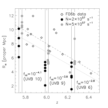
Figure 8: The sizes of Ly$\alpha$ near-zones as a function of redshift. The filled black circles correspond to the individual Ly$\alpha$ near-zone sizes taken from the synthetic spectra in the moderate evolution scenario. Here the quasar is assumed to have an ionizing luminosity of $\dot{N}=2\times 10^{57}\rm~{}s^{-1}$. The observed correlation between Ly$\alpha$ near-zone size and redshift, determined empirically by Fan et al. (2006b), is shown with the dashed line. This fit has been made with observed Ly$\alpha$ near-zone sizes rescaled to a common quasar ionizing luminosity of $\sim 1.9\times 10^{57}\rm~{}s^{-1}$, which are shown by the open diamonds. The simulation data lie slightly below this fit, although the evolutionary trend is roughly similar. The filled grey circles correspond to the same synthetic sight-lines, except now the quasar ionizing luminosity is increased to $\dot{N}=5\times 10^{57}\rm~{}s^{-1}$. These data are in somewhat better agreement with the fit to the observational data. Note that the solid vertical lines are to guide the eye only. In addition, only four data points are visible for the $\dot{N}=2\times 10^{57}\rm~{}s^{-1}$ data at $z=6.25$ and $z=5.75$. In these instances two near-zones have been measured to have the same size.

We now compare the absolute sizes of the synthetic Ly$\alpha$ near-zones with the observations of F06b. In figure 8 we plot the individual Ly$\alpha$ near-zone sizes used in the moderate evolution scenario against redshift as filled black circles, similar to figure 12 in F06b. The dashed line is the empirically determined correlation between $R_{\alpha}$ and redshift quoted by F06b. The dotted line is the same relation assuming the observed near-zone redshifts were overestimated by $\Delta z=0.02$, which is the uncertainty quoted by F06b. The observed Ly$\alpha$ near-zone sizes from which this fit is derived in F06b, shown by the open diamonds in figure 8, are rescaled to a common absolute magnitude of $M_{1450}=-27$, assuming $\dot{N}\propto M_{1450}$ and $R_{\alpha}\propto\dot{N}^{1/3}$. This is an uncertain correction and a rescaling by $\dot{N}^{1/2}$ may actually be more appropriate. Using the spectral energy distribution given by equation (14), $M_{1450}=-27$ corresponds to $\dot{N}=1.9\times 10^{57}\rm~{}s^{-1}$, which is close to the fiducial value of $\dot{N}=2\times 10^{57}\rm~{}s^{-1}$ adopted for this study. We also note briefly the linear fit to the observational data shown in figure 12 of F06b is given by $R_{\alpha}=8-9(z-6)\rm~{}Mpc$, which is reproduced in our figure 8. This is slightly different to equation (24) in F06b, which they quoted erroneously (X. Fan, private communication).

Interestingly, we obtain Ly$\alpha$ near-zone sizes which are 20-50 per cent smaller than the observational data. The relative evolution and scatter in the near-zone sizes is broadly consistent with the F06b results. This may indicate that the actual density and temperature distribution of the IGM is somewhat different from that in our numerical simulations and that the actual mean neutral fraction is somewhat smaller than we have assumed for the simulated spectra. Another obvious way of reconciling the synthetic near-zone sizes of our moderate evolution scenario with the observational data is to increase the ionizing flux in the the near-zone. The filled grey circles in figure 8 correspond to the same synthetic sight-lines, except now the quasar ionizing luminosity is set to $\dot{N}=5\times 10^{57}\rm~{}s^{-1}$, a factor of 2.5 larger than before. The near-zone sizes are now in better agreement with the observational data. However, it appears unlikely that the observed quasar luminosities are underestimated by a factor of two to three. If an enhanced ionizing luminosity really were required to reproduce the absolute sizes of observed Ly$\alpha$ near-zones, this may instead be attributed to star forming galaxies which are likely to cluster in the dense environment surrounding the quasar.

Recently, Yu & Lu (2005) suggested that the majority of the neutral hydrogen surrounding a quasar may have already been ionized by stellar sources before the quasar switches on. However, a factor three larger ionizing luminosity appears again too large, considering quasars are already extremely luminous objects. There is, however, an important effect which our simulations do not take into account which can increase the combined ionizing flux from galaxies (and faint quasars) in the near-zone without an enhanced ionizing luminosity from individual galaxies. The enhanced ionizing flux from the quasar in the near-zone will ionize dense neutral regions which otherwise block the ionizing radiation from other sources of ionizing photons. This leads to a significant increase of the ionizing photon mean free path within the near-zone compared to the mean free path in the surrounding IGM. This will lead to an increase in the metagalactic UV background flux due to the galaxies and possibly other, fainter quasars within the near-zone. An accurate estimate of this effect is difficult but a rough estimate can be obtained using our SSC model (Miralda-Escudé et al. 2000; Furlanetto & Oh 2005, and also see appendix D). An increase by a factor of two or three in the ionizing flux at the edge of the near-zone appears plausible.

There is a range of other effects which may affect the estimated near-zone sizes. However, they should be less important than the effects discussed above. Spatial fluctuations in the UV background expected around the end of reionization may influence the size of observed near-zones. In addition, gas in highly overdense regions is likely to be shocked, producing hot, highly ionized gas. This has not been taken account in our simulations. However, the volume filling factor of this hot, ionized gas phase is expected to be small at $z=6$. The difficulty of the data reduction may also contribute to the discrepancy. The continuum fitting of these highly absorbed spectra in the region of the broad Ly$\alpha$ emission line is notoriously difficult. Unidentified emission lines could easily lead to a quasar continuum which is placed too low at the relevant distance from the systemic redshift. This would result in an overestimate of the transmission and could therefore result in an overestimate of the observed near-zone sizes.

6 Conclusions and discussion

We have presented a detailed investigation of the properties of near-zones in the Lyman series absorption spectra of $z\simeq 6$ quasars, using analytical estimates and an accurate radiative transfer scheme for a hydrogen and helium IGM combined with density distributions drawn from a large hydrodynamical simulation of a $\Lambda$CDM universe. From the radiative transfer simulations we have produced realistic mock spectra which we have analysed in a similar manner to the current observational data. The main conclusions of this study are as follows.

$\bullet$ For large IGM neutral hydrogen fractions the size of the near-zone increases as $f_{\rm HI}^{-1/3}$, as expected for an H $\rm\scriptstyle II\$I-front expanding into a significantly neutral medium. For typical luminosities of observed $z\simeq 6$ quasars and plausible lifetimes, the near-zone sizes saturate at a neutral fraction $f_{\rm HI}\approx 0.1$. For smaller neutral fractions the spectroscopically identified near-zones are more akin to classical proximity zones within a highly ionized IGM, and their size is largely independent of the neutral hydrogen fraction of the surrounding IGM.

$\bullet$ The density fluctuations in a cosmologically representative matter distribution lead to considerable scatter in the size of the near-zones, even for fixed assumptions about the ionization state of the surrounding IGM. It is thus difficult to determine the IGM neutral hydrogen fraction from a small number of observed spectra.

$\bullet$ Observed sizes of spectroscopically identified near-zones in the Ly$\alpha$ region alone are a rather poor indicator of the ionization state of the surrounding IGM. Observed near-zone sizes can furthermore substantially underestimate the size of the region impacted by the ionizing radiation of the quasar.

$\bullet$ For small neutral hydrogen fractions quasar He $\rm\scriptstyle III\$I-fronts lag considerably behind their H $\rm\scriptstyle II\$counterparts if He $\rm\scriptstyle II\$is still abundant. This leads to a temperature jump behind the He $\rm\scriptstyle III\$I-front which can be located within the observed near-zone for a suitable combination of IGM neutral fraction, quasar luminosity and quasar lifetime. Detailed study of the width of the absorption features in the Ly$\alpha$ near-zone may therefore reveal the position of the He $\rm\scriptstyle III\$front. This could then be used together with the Ly$\alpha$ near-zone size to constrain the neutral hydrogen fraction.

$\bullet$ The ratio of near-zone sizes in the Ly$\alpha$ and Ly$\beta$ region of quasar spectra provides another independent probe of the ionization state of the surrounding IGM. For neutral fractions $f_{\rm HI}\geq 10^{-2}$ we find that the size of the Ly$\alpha$ and Ly$\beta$ near-zones are similar. For smaller neutral fractions the size of the Ly$\beta$ region becomes substantially larger, approaching the theoretical limit of $R_{\beta}\simeq 2.5R_{\alpha}$. The extent of the Ly$\beta$ near-zone relative to Ly$\alpha$ is blurred by the overlying Ly$\alpha$ forest at lower redshift. It is also very sensitive to the density distribution along the line-of-sight. For this reason the ratio of the sizes of the Ly$\alpha$ and Ly$\beta$ near-zones approaches the saturated value at a neutral fraction somewhat smaller ($f_{\rm HI}\la 10^{-2}$) than where saturation sets in for the sizes of Ly$\alpha$ near-zones alone ($f_{\rm HI}\sim 10^{-1}$). The exact value of the threshold neutral hydrogen fractions depends on the quasar luminosity and lifetime.

$\bullet$ The synthetic spectra produced from our radiative transfer simulations exhibit Ly$\alpha$ near-zones which are $20-50$ per cent smaller than the observed spectra for plausible assumptions for the ionizing luminosity of the the quasar and the flux of the metagalactic UV background in the surrounding IGM. The discrepancy is resolved if the ionizing flux at the edge of the near-zone is enhanced by a factor of two to three. Such an enhancement is plausible given the expected increase in the ionizing photon mean free path in the near-zone compared to the mean free path in the surrounding IGM. This would produce a corresponding enhancement of the metagalactic UV background within the near-zone from stellar emission and possibly fainter quasars. Alternatively, it may suggest that the IGM has a lower neutral fraction than we assumed in our simulations.

$\bullet$ The strong evolution of the observed sizes of Ly$\alpha$ near-zones over the short redshift interval $5.7<z<6.4$ is consistent with, but does not require, a rapid evolution of the neutral hydrogen fraction of the surrounding IGM. The observed evolution in the Ly$\alpha$ near-zone size by around a factor of two is equally consistent with a moderate evolution in the IGM neutral hydrogen fraction. Relatively small changes in the highly ionized IGM neutral hydrogen fraction can produce a rapid evolution in the observed sizes of Ly$\alpha$ near-zones if the ionizing flux from the quasar at the edge of the near-zone is comparable to the flux of the metagalactic UV background at the Lyman limit in the surrounding IGM. In this case the rapid evolution can be attributed to additional transmission from the thinning Ly$\alpha$ forest. This proposition can be tested by varying the flux level used to define the extent of the near-zone sizes. For larger flux levels the evolution should decrease if the increasing transmission from the general Ly$\alpha$ forest is responsible for part or most of the evolution.

$\bullet$ The effect of self-shielded clumps on the observed sizes of the Ly$\alpha$ near-zone is small, and the expected evolution of the incidence rate of self-shielded clumps appears to contribute little to the rapid evolution of near-zone sizes.

We note here that we have not considered two further possibilities which may influence the size of quasar near-zones: a fluctuating UV background and additional sources of ionizing radiation, such as star forming galaxies, clustered in the vicinity of the quasar host halo. Both of these are likely to increase the observed near-zone sizes. Additionally, observational constraints on near-zone sizes are still somewhat uncertain, as are quasar ionizing luminosities and lifetimes. However, a large sample of high quality quasar spectra with an accurate determination of the sizes of the Ly$\alpha$ and Ly$\beta$ near-zones should improve the constraints on the ionization state of the IGM at $z>6$ considerably. If most quasars exhibit Ly$\beta$ near-zones which are similar in size to the counterpart Ly$\alpha$ near-zone, this should favour an IGM with $f_{\rm HI}\geq 10^{-2}$. If Ly$\beta$ near-zones were instead generally larger than their Ly$\alpha$ counterparts this would provide evidence for an IGM with $f_{\rm HI}\leq 10^{-2}$. The information locked within the widths of absorption features in the Ly$\alpha$ near-zones may provide an interesting additional probe of the ionization state of the IGM at high redshift.

Appendix A Time delay effects on observed sizes of cosmological H $\rm\scriptstyle II\$regions

The existence of a finite speed for the transmission of real information alters the observed sizes and shapes of cosmological H $\rm\scriptstyle II\$regions. These time delay effects, although having their basis in special relativity with the postulate that the speed of light in empty space always has the same value, are purely geometrical rather than relativistic phenomena which manifest themselves when the I-fronts travel at relativistic speeds. The renewed interest in cosmological H $\rm\scriptstyle II\$regions as a probe of the epoch of reionization has meant these effects have been well documented within the recent literature, to which we refer the interested reader (e.g. White et al. 2003; Yu & Lu 2005; Yu 2005; Shapiro et al. 2006) However, we briefly review these results here, as they provide an important simplification to our radiative transfer scheme.

One can easily show the expression for the radius, $R$, of a H $\rm\scriptstyle II\$region expanding into a static, pure hydrogen medium of constant density and temperature is (e.g. Wyithe & Loeb 2004; Shapiro et al. 2006)

$$\frac{dR}{dt}=c\left[\frac{\dot{N}-\frac{4}{3}\pi R^{3}\alpha_{\rm HII}n_{\rm H}^{2}}{\dot{N}+4\pi R^{2}f_{\rm HI}n_{\rm H}c-\frac{4}{3}\pi R^{3}\alpha_{\rm HII}n_{\rm H}^{2}}\right],$$ (17)

where $\dot{N}$ is the number of ionizing photons emitted by the monochromatic source per unit time, $n_{\rm H}$ is the number density of hydrogen atoms, $f_{\rm HI}=n_{\rm HI}/n_{\rm H}$ is the neutral hydrogen fraction and $\alpha_{\rm HII}$ is the recombination coefficient for ionized hydrogen. This expression explicitly takes into account the time delay for a photon to travel from the source to the edge of the H $\rm\scriptstyle II\$region, thus setting the limiting expansion speed of the H $\rm\scriptstyle II\$region to the speed of light.

Now consider the expansion of a H $\rm\scriptstyle II\$region outwards from the ionizing source along the line of sight to an observer. Any photons instantaneously detected by the observer were emitted at the same retarded time, $t_{\rm R}=t-R/c$, where $t$ is the time when the photons reach a distance $R$ from the source. Evaluating equation 17 at the retarded time yields

$$\frac{dR}{dt_{\rm R}}=\frac{\dot{N}-\frac{4}{3}\pi R^{3}\alpha_{\rm HII}n_{\rm H}^{2}}{4\pi R^{2}f_{\rm HI}n_{\rm H}},$$ (18)

which is identical to equation (1). Thus, it is clear for this particular geometrical configuration that the expansion speed of the H $\rm\scriptstyle II\$region in the observer’s frame is no longer limited to the speed of light; it is as if one can completely ignore time delay effects and assume real information is transmitted instantaneously. This leads to the observation of an initial superluminal expansion phase close to the ionizing source, when the number of ionizing photons per hydrogen atom at the I-front greatly exceeds unity, allowing it to propagate at relativistic speeds. This result is particularly useful in the context of our radiative transfer simulations, which we discuss in the next section.

Appendix B Radiative transfer implementation

Modelling the extent of cosmological H $\rm\scriptstyle II\$regions around high redshift quasars, while consistently tracking local changes in the ionization state and temperature of the gas due to the filtering of ionizing radiation, requires a full treatment of radiative transfer through a hydrogen and helium IGM. In a cosmologically expanding medium I-fronts from a luminous quasar are highly supersonic and thus decoupled from the hydrodynamical response of the gas. This allows one to ignore the radiation hydrodynamics of this particular problem, providing a significant simplification to our numerical scheme. For this purpose we use an updated version of the radiative transfer algorithm of Bolton et al. (2004). This algorithm is based on the explicit photon conservation method of Abel et al. (1999), which has the desirable property that photons are conserved almost independently of spatial resolution, allowing the accurate determination of physically relevant quantities with only moderate computational expense. We briefly outline the updated algorithm here and then present some tests of the code.

B.1 The cosmological model

We adopt the following time-redshift relation for a flat Universe dominated by a cosmological constant and non-relativistic matter (Peebles 1993)

$$H_{0}t=\frac{2}{3(1-\Omega_{\rm m})^{1/2}}\sinh^{-1}\left[\left(\frac{1-\Omega_{\rm m}}{\Omega_{\rm m}}\right)^{1/2}a^{3/2}\right],$$ (19)

where $H_{0}=100h~{}\rm km~{}s^{-1}~{}Mpc^{-1}$ is the present day Hubble parameter, $\Omega_{\rm m}$ is the matter density as a fraction of the critical density and $a=(1+z)^{-1}$ is the cosmological scale factor. We use this relation to update redshift dependent quantities at each successive timestep $\delta t$ within the radiative transfer implementation. Additionally, from equation (19) it is straightforward to derive an expression for the Hubble parameter

$$H(t)=\Omega_{\rm m}^{1/2}H_{0}\cosh\left[\frac{3H_{0}}{2}(1-\Omega_{\rm m})^{1/2}t\right]a^{-3/2}.$$ (20)

B.2 The ionizing radiation field

Consider a source which emits $\dot{N}$ ionizing photons per unit time, such that

$$\dot{N}=\int_{\nu_{\rm HI}}^{\infty}\dot{N}_{\nu}d\nu=\int_{\nu_{\rm HI}}^{\infty}\frac{L_{\nu}}{h_{\rm p}\nu}d\nu,$$

where $L_{\nu}~{}d\nu$ is the luminosity of the source within the frequency interval $\nu\rightarrow\nu+d\nu$, defined as

$$L_{\nu}~{}d\nu=L_{\rm HI}\left(\frac{\nu}{\nu_{\rm HI}}\right)^{-\alpha_{\rm s}}d\nu.$$

The source has a power law spectrum with index $\alpha_{\rm s}$, typical of quasars, normalised by $L_{\rm HI}$ at the H $\rm\scriptstyle I\$ionization threshold frequency, $\nu_{\rm HI}$.

The probabilities of an ionizing photon emitted by the source then being absorbed by H $\rm\scriptstyle I$, He $\rm\scriptstyle I\$and He $\rm\scriptstyle II$, respectively, are (Bolton et al. 2004)

$$P_{\rm HI}=p_{\rm HI}q_{\rm HeI}q_{\rm HeII}(1-{\rm e}^{-\tau_{\nu}^{\rm tot}})/D,$$

$$P_{\rm HeI}=q_{\rm HI}p_{\rm HeI}q_{\rm HeII}(1-{\rm e}^{-\tau_{\nu}^{\rm tot}})/D,$$

$$P_{\rm HeII}=q_{\rm HI}q_{\rm HeI}p_{\rm HeII}(1-{\rm e}^{-\tau_{\nu}^{\rm tot}})/D,$$

where $p_{\rm i}=1-{\rm e}^{-\tau_{\nu}^{\rm i}}$, $q_{\rm i}={\rm e}^{-\tau_{\nu}^{\rm i}}$, $\tau_{\nu}^{\rm tot}=\tau_{\nu}^{\rm HI}+\tau_{\nu}^{\rm HeI}+\tau_{\nu}^{\rm HeII}$, $\tau_{\nu}^{i}$ is the optical depth for species $i$ and $D=p_{\rm HI}q_{\rm HeI}q_{\rm HeII}+q_{\rm HI}p_{\rm HeI}q_{\rm HeII}+q_{\rm HI}q_{\rm HeI}p_{\rm HeII}$.

If we now invoke a uniformly discretised space grid with elements of size $\delta R$ along the line-of-sight to the source, at any given timestep $\delta t$, the photo-ionization rate per unit volume $\rm[s^{-1}~{}cm^{-3}]$ of species $i$ in grid element $l$ is

$$n_{\rm i}^{\rm l}\Gamma_{\rm i}^{\rm l}=\frac{1}{V^{\rm l}}\int_{\nu_{\rm i}}^{\infty}\dot{N}_{\nu}^{\rm l-1}P_{\rm i}~{}d\nu,$$

where $V^{\rm l}$ is the volume of element $l$ and $\nu_{\rm i}$ is the ionization threshold frequency for species $i$. If we assume the luminosity of the source is constant and allow an additional contribution to the ionization rate from a diffuse UV background, the above equation can be rewritten as

$$n_{\rm i}^{\rm l}\Gamma_{\rm i}^{\rm l}=\left[\frac{1}{4\pi R^{2}\delta R}\sum_{k}\frac{L_{\nu_{\rm k}}}{h_{\rm p}\nu_{\rm k}}P_{\rm i}e^{-T_{\nu_{\rm k}}}\right]+n_{\rm i}^{\rm l}\Gamma_{\rm i}^{\rm b},$$ (21)

which is the equation we shall solve for the ionization rate per unit volume for species $\rm i$. Here we have optimally discretised the frequency integration into $20$ logarithmically spaced intervals $k$ between $\nu_{\rm i}$ and $10\nu_{\rm i}$, $R$ is the distance of element $l$ from the source, $\Gamma_{\rm i}^{\rm b}$ is the optically thin photo-ionization rate due to the diffuse metagalactic UV background and the transmission factor, $T_{\nu}$, is defined as

$$T_{\nu}=\cases{0&($l=0$),\cr\vskip 3.0pt\cr\sum_{j=0}^{l-l}(\sigma_{\rm HI}n_{\rm HI}^{j}+\sigma_{\rm HeI}n_{\rm HeI}^{j}+\sigma_{\rm HeII}n_{\rm HeII}^{j})\delta R&($l>0$).\cr}$$

Similarly, the photo-heating rate per unit volume $\rm[erg~{}s^{-1}~{}cm^{-3}]$ for species $i$ is given by

$$n_{\rm i}^{\rm l}{\epsilon}_{\rm i}^{\rm l}=\left[\frac{1}{4\pi R^{2}\delta R}\sum_{\rm k}\frac{L_{\nu_{\rm k}}}{h_{\rm p}\nu_{\rm k}}P_{\rm i}h_{\rm p}(\nu_{\rm k}-\nu_{\rm i})e^{-T_{\nu_{\rm k}}}\right]+n_{\rm i}^{\rm l}\epsilon_{\rm i}^{\rm b},$$ (22)

such that the total photo-heating rate per unit volume in element $l$ is given by ${\mathscr{H}}_{\rm tot}^{l}=n_{\rm HI}\epsilon_{\rm HI}^{\rm l}+n_{\rm HeI}\epsilon_{\rm HeI}^{\rm l}+n_{\rm HeII}\epsilon_{\rm HeII}^{\rm l}$ and $\epsilon_{\rm i}^{\rm b}$ is the optically thin photo-heating rate due to the diffuse UV background.

In general, for each timestep $\delta t$ the number densities $n_{\rm i}$ in the expression for the transmission factor $T_{\nu}$ are evaluated in each grid cell $j$ at the same retarded time $t_{\rm R}=t-j\delta R/c$, where $t$ is the time it takes a light signal to reach cell $j$. In principle, an I-front propagating outwards from the source is then limited to travel no faster than the speed of light since $n_{\rm i}$ are only evaluated when $t\geq j\delta R/c$. However, in practice spatial discretisation means this is not always the case; an I-front is assumed to propagate instantaneously across a cell width $\delta R$. Even for relatively high spatial resolution, this enables the expansion rate of the ionized region to exceed $c$. This means that to accurately compute the position of an I-front one must either increase the spatial resolution to a prohibitively high level or artificially impose the limit $R\leq ct$. At first glance, the latter option would seem to be preferable. However, this has the undesirable effect of violating photon conservation, so that although one correctly predicts the position of the I-front (e.g. Abel et al. 1999), one must again resort to substantially higher spatial resolution (such that each cell in the space grid is optically thin) to compute physically relevant quantities within the region where $R\leq ct$ is imposed. This is a problem for simulating quasar near-zones in Lyman series absorption, since the absorption spectrum is sensitive to the exact values of the neutral fraction and temperature of the gas near the source. Fortunately, we have already shown that in the frame of an observer the expansion rate of the I-front follows equation (18). Since we are interested in the sizes of observed H $\rm\scriptstyle II\$regions, we may evaluate the expression for $T_{\nu}$ assuming the photons are transmitted instantaneously, removing the need to impose the condition $R\leq ct$ while at the same time explicitly conserving photons. This enables us to determine the ionized fraction and temperature of the gas close to the ionizing source accurately for relatively coarse spatial resolution, substantially reducing the computational expense of the simulations.

B.3 Computing the ionized fraction and temperature

At every timestep $\delta t$, in each spatial grid element $\delta R$, the ionization state and temperature of atomic hydrogen and helium must be computed by solving a set of four coupled first order ordinary differential equations. The first three determine the abundances of the three ionized species

$$\frac{dn_{\rm HII}}{dt}=n_{\rm HI}(\Gamma_{\rm HI}+n_{\rm e}\Gamma_{\rm eHI})-n_{\rm HII}n_{\rm e}\alpha_{\rm HII},$$ (23)

$$\frac{dn_{\rm HeII}}{dt}=n_{\rm HeI}(\Gamma_{\rm HeI}+n_{e}\Gamma_{\rm eHeI})+n_{\rm HeIII}n_{\rm e}\alpha_{\rm HeIII}$$

$$\hskip 28.45274pt-n_{\rm HeII}(\Gamma_{\rm HeII}+n_{\rm e}\Gamma_{\rm eHeII}+n_{\rm e}\alpha_{\rm HeII}),$$ (24)

$$\frac{dn_{\rm HeIII}}{dt}=n_{\rm HeII}(\Gamma_{\rm HeII}+n_{\rm e}\Gamma_{\rm eHeII})-n_{\rm HeIII}n_{\rm e}\alpha_{\rm HeIII},$$ (25)

with the closing conditions

$$n_{\rm HI}=n_{\rm H}-n_{\rm HII},$$

$$n_{\rm HeI}=\frac{Y}{4(1-Y)}n_{\rm H}-n_{\rm HeII}-n_{\rm HeIII},$$

$$n_{\rm e}=n_{\rm HII}+n_{\rm HeII}+2n_{\rm HeIII}.$$

Here $n_{\rm i}$ denotes the number density $[\rm cm^{-3}]$ of species $i$, $\Gamma_{\rm i}$ $[\rm s^{-1}]$ is the photo-ionization rate, $\Gamma_{\rm ei}$ $[\rm cm^{3}~{}s^{-1}]$ is the collisional ionization rate, $\alpha_{\rm i}$ $[\rm cm^{3}~{}s^{-1}]$ is the total radiative recombination coefficient and $Y$ is the helium mass fraction, which we take to be $Y=0.24$ (e.g. Olive & Skillman 2004).

Additionally, the temperature must also be computed by solving a fourth differential equation

$$\frac{dT}{dt}=\frac{(\gamma-1)\mu m_{\rm H}}{k_{\rm B}\rho}[{\mathscr{H}}_{\rm tot}-\Lambda(n_{\rm i},T)]-2H(t)T,$$ (26)

where $\mu$ is the mean molecular weight of the gas, $\gamma=5/3$, $\Lambda(n_{\rm i},T)$ $\rm[erg~{}s^{-1}~{}cm^{-3}]$ is the radiative cooling function, $H(t)$ is the Hubble parameter given by equation (20) and all other symbols have their usual meanings. The last term on the right hand side of equation (26) is the contribution to cooling by the adiabatic expansion of the Universe.

We solve equations (23)-(26) using a first order implicit integration scheme which provides a good balance between accuracy and speed (Anninos et al. 1997). We find that to solve these equations accurately, one must typically adopt a timestep comparable to the hydrogen ionization timescale, $t_{\rm ion}=1/\Gamma_{\rm HI}$, which can become very small in close proximity to a luminous source. On occasion this time interval is smaller than the main timestep we use to track the position of the I-front (see section C.1 for details). When this is the case we sub-cycle over each main time step using smaller time intervals based on the ionization timescale to solve for the ionic abundances. Once the rate of change in the electron number density is less than $10^{-8}$, we switch to solving the ionic abundances assuming the gas is in ionization equilibrium (e.g. Katz et al. 1996). This leaves only the differential equation for the temperature to be integrated, allowing much larger timesteps to be taken which greatly speeds up the calculation.

B.4 Cross-sections and rates

The cross-sections and rates adopted in our radiative transfer scheme are listed below. Note that we use case A instead of case B recombination coefficients for this study. For optically thick hydrogen and helium, one can approximately take into account the moderate boost to the photo-ionization rates due to diffuse radiation emitted by recombining ions using case B recombination coefficients. This is the so-called on-the-spot approximation (Spitzer 1978). However, any gas seen in Ly$\alpha$ absorption in our simulated spectra typically lies behind the source I-fronts and is thus optically thin. In addition, for typical gas densities the recombination timescale is considerably longer than the canonical quasar lifetime. In these circumstances we find case A recombination coefficients are the appropriate choice.

(1) Photo-ionization cross-sections $[\rm cm^{2}]$ (Osterbrock 1989):

$$\sigma_{\rm HI}=6.30\times 10^{-18}[1.34(\nu/\nu_{\rm HI})^{-2.99}-0.34(\nu/\nu_{\rm HI})^{-3.99}],$$

$$\sigma_{\rm HeI}=7.03\times 10^{-18}[1.66(\nu/\nu_{\rm HeI})^{-2.05}-0.66(\nu/\nu_{\rm HeI})^{-3.05}],$$

$$\sigma_{\rm HeII}=1.50\times 10^{-18}[1.34(\nu/\nu_{\rm HeII})^{-2.99}-0.34(\nu/\nu_{\rm HeII})^{-3.99}].$$

(2) Optically thin photo-ionization rates $[\rm s^{-1}]$:

$$\Gamma_{\rm HI}^{\rm b}=1.27\times 10^{-11}J_{-21}^{\rm b}(\alpha_{\rm b}+3)^{-1},$$

$$\Gamma_{\rm HeI}^{\rm b}=1.51\times 10^{-11}(0.553)^{\alpha_{\rm b}}J_{-21}^{\rm b}(\alpha_{\rm b}+2)^{-1},$$

$$\Gamma_{\rm HeII}^{\rm b}=3.03\times 10^{-12}(0.250)^{\alpha_{\rm b}}J_{-21}^{\rm b}(\alpha_{\rm b}+3)^{-1},$$

where the specific intensity of the metagalactic radiation field $\rm[erg~{}s^{-1}~{}cm^{-2}sr^{-1}Hz^{-1}]$ is defined as

$$J_{\nu}^{\rm b}=J_{-21}^{\rm b}\times 10^{-21}\left(\frac{\nu}{\nu_{\rm HI}}\right)^{-\alpha_{\rm b}}.$$

The radiation field is assumed to have a power law spectrum with index $\alpha_{\rm b}$, normalised by $J_{-21}^{\rm b}$ at the $\rm HI$ ionization threshold.

(3) Optically thin photo-heating rates $[\rm erg~{}s^{-1}]$:

$$\epsilon_{\rm HI}^{\rm b}=2.94\times 10^{-22}J_{-21}^{\rm b}[(\alpha_{\rm b}+2)(\alpha_{\rm b}+3)]^{-1},$$

$$\epsilon_{\rm HeI}^{\rm b}=6.48\times 10^{-22}(0.553)^{\alpha_{\rm b}}J_{-21}^{\rm b}[(\alpha_{\rm b}+1)(\alpha_{\rm b}+2)]^{-1},$$

$$\epsilon_{\rm HeII}^{\rm b}=2.80\times 10^{-22}(0.250)^{\alpha_{\rm b}}J_{-21}^{\rm b}[(\alpha_{\rm b}+2)(\alpha_{\rm b}+3)]^{-1}.$$

(2) Recombination rates $[\rm cm^{3}~{}s^{-1}]$ (Abel et al. 1997):

$$\alpha_{\rm HII}=\exp(-28.6130338-0.72411256\ln(\tilde{T})$$

$$\hskip 19.91692pt-2.02604473\times 10^{-2}\ln(\tilde{T})^{2}-2.38086188\times 10^{-3}\ln(\tilde{T})^{3}$$

$$\hskip 19.91692pt-3.21260521\times 10^{-4}\ln(\tilde{T})^{4}-1.42150291\times 10^{-5}\ln(\tilde{T})^{5}$$

$$\hskip 19.91692pt+4.98910892\times 10^{-6}\ln(\tilde{T})^{6}+5.75561414\times 10^{-7}\ln(\tilde{T})^{7}$$

$$\hskip 19.91692pt-1.85676704\times 10^{-8}\ln(\tilde{T})^{8}-3.07113524\times 10^{-9}\ln(\tilde{T})^{9},$$

$$\alpha_{\rm HeII}=\alpha_{\rm HeII}^{\rm r}+\alpha_{\rm HeII}^{\rm d},$$

$$\alpha_{\rm HeII}^{\rm r}=3.925\times 10^{-13}\tilde{T}^{-0.6353},$$

$$\alpha_{\rm HeII}^{\rm d}=1.544\times 10^{-9}\tilde{T}^{-1.5}{\rm e}^{-48.596/\tilde{T}}(0.3+{\rm e}^{8.1/\tilde{T}}),$$

$$\alpha_{\rm HeIII}=2\alpha_{\rm HII}(\tilde{T}/4),$$

where $\tilde{T}$ is the gas temperature in electron volts.

(4) Collisional ionization rates $[\rm cm^{3}~{}s^{-1}]$ (Theuns et al. 1998):

$$\Gamma_{\rm eHI}=1.17\times 10^{-10}T^{0.5}{\rm e}^{-157809.1/T}[1+T_{5}^{1/2}]^{-1},$$

$$\Gamma_{\rm eHeI}=4.76\times 10^{-11}T^{0.5}{\rm e}^{-285335.4/T}[1+T_{5}^{1/2}]^{-1},$$

$$\Gamma_{\rm eHeII}=1.14\times 10^{-11}T^{0.5}{\rm e}^{-631515.0/T}[1+T_{5}^{1/2}]^{-1},$$

where $T_{5}=T/10^{5}\rm~{}K$.

The following radiative cooling processes contribute towards the cooling function $\Lambda(n_{\rm i},T)$:

(5) Recombination cooling $[\rm erg~{}s^{-1}~{}cm^{-3}]$:

$$\Lambda_{\rm HII}^{\rm rec}=1.036\times 10^{-16}T\alpha_{\rm HII}n_{\rm e}n_{\rm HII},$$

$$\Lambda_{\rm HeII}^{\rm rec}=(1.036\times 10^{-16}T\alpha_{\rm HeII}^{\rm r}+6.526\times 10^{-11}\alpha_{\rm HeII}^{\rm d})n_{\rm e}n_{\rm HeII},$$

$$\Lambda_{\rm HeIII}^{\rm rec}=1.036\times 10^{-16}T\alpha_{\rm HeIII}n_{\rm e}n_{\rm HeIII}.$$

(6) Collisional ionization cooling $[\rm erg~{}s^{-1}~{}cm^{-3}]$ (Theuns et al. 1998):

$$\Lambda_{\rm eHI}=2.18\times 10^{-11}\Gamma_{\rm eHI}n_{\rm e}n_{\rm HI},$$

$$\Lambda_{\rm eHeI}=3.94\times 10^{-11}\Gamma_{\rm eHeI}n_{\rm e}n_{\rm HeI},$$

$$\Lambda_{\rm eHeII}=8.72\times 10^{-11}\Gamma_{\rm eHeII}n_{\rm e}n_{\rm HeII}.$$

(7) Collisional excitation cooling $[\rm erg~{}s^{-1}~{}cm^{-3}]$ (Cen 1992):

$$\Lambda_{\rm HI}^{\rm ex}=7.50\times 10^{-19}{\rm e}^{-118348/T}[1+T_{5}^{1/2}]^{-1}n_{\rm e}n_{\rm HI},$$

$$\Lambda_{\rm HeI}^{\rm ex}=9.10\times 10^{-27}T^{-0.1687}{\rm e}^{-13179.0/T}[1+T_{5}^{1/2}]^{-1}n_{\rm e}^{2}n_{\rm HeI},$$

$$\Lambda_{\rm HeII}^{\rm ex}=5.54\times 10^{-17}T^{-0.397}{\rm e}^{-473638/T}[1+T_{5}^{1/2}]^{-1}n_{\rm e}n_{\rm HeII}.$$

(8) Bremsstrahlung $[\rm erg~{}s^{-1}~{}cm^{-3}]$ (Cen 1992):

$$\Lambda_{\rm ff}=1.43\times 10^{-27}T^{1/2}g_{\rm ff}(n_{\rm HII}+n_{\rm HeII}+4n_{\rm HeIII})n_{\rm e},$$

where the Gaunt factor for free-free emission, $g_{\rm ff}$, is given by

$$g_{\rm ff}=1.1+0.34\exp[-(5.5-\log_{10}(T)]^{2}.$$

(9) Inverse Compton cooling $[\rm erg~{}s^{-1}~{}cm^{-3}]$ (Peebles 1971):

$$\Lambda_{\rm c}=5.65\times 10^{-36}[T-2.73(1+z)](1+z)^{4}n_{\rm e}.$$

Appendix C Code tests

Figure 9: Test of spatial convergence for our radiative transfer scheme. The left hand panels show the fractional abundances of H $\rm\scriptstyle I$, He $\rm\scriptstyle II\$and the gas temperature for model A using the cell sizes labelled on the plot. The right hand panels show the same quantities for model B.

Figure 10: Test of temporal convergence for our radiative transfer scheme. The left hand panels show the fractional abundances of H $\rm\scriptstyle I$, He $\rm\scriptstyle II\$and the gas temperature for model A using the Courant conditions labelled on the plot. The right hand panels show the same quantities for model B.

Exploring the limitations of any numerical model is essential for providing well motivated results. To this end we present some selected tests of the radiative transfer implementation we use for our simulations. The test models are summarised in table LABEL:tab:models

Table 4: Radiative transfer test models. For each model the columns list the ionizing photon production rate of the source $\dot{N}$, the spectral index of the source $\alpha_{\rm s}$, the hydrogen number density $n_{\rm H}$, the mass fraction of helium $Y$ and the age of the source $t_{\rm s}$. Models C and D are for a monochromatic source, therefore no source spectral indices are listed.

Model	$\dot{N}\rm~{}[s^{-1}]$	$\alpha_{\rm s}$	$n_{\rm H}\rm~{}[cm^{-3}]$	$Y$	$t_{\rm s}\rm~{}[yrs]$
A	$5\times 10^{53}$	$1.5$	$7\times 10^{-5}$	0.24	$10^{6}$
B	$5\times 10^{56}$	$1.5$	$7\times 10^{-2}$	0.24	$10^{6}$
C	$1\times 10^{55}$	$-$	$7\times 10^{-5}$	0	$10^{7}$
D	$1\times 10^{59}$	$-$	$7\times 10^{-2}$	0	$10^{7}$

C.1 Spatial and temporal resolution requirements

We firstly present some convergence tests for the spatial and temporal resolution of our radiative transfer scheme. Our algorithm has the useful property that photons are conserved explicitly independent of spatial resolution (e.g. Abel et al. 1999; Bolton et al. 2004; Mellema et al. 2006). Consequently, the ionized fraction and temperature are computed accurately even when the cells on the space grid are very optically thick, speeding the calculation up considerably.

The optical depth to neutral hydrogen in each cell of width $\delta R$ on the space grid is given by $\delta\tau_{\rm HI}=\sigma_{\rm HI}n_{\rm HI}\delta R$. Employing fiducial values, this can be written as

$$\delta\tau_{\rm HI}=13.6\left(\frac{n_{\rm HI}}{7\times 10^{-5}\rm~{}cm^{-3}}\right)\left(\frac{\delta R}{10\rm~{}kpc}\right).$$ (27)

Note that in the case of a hydrogen and helium IGM, the optical depth to He $\rm\scriptstyle I\$and He $\rm\scriptstyle II\$per cell is less than that for H $\rm\scriptstyle I\$due to the lower number density of these species and, in the case of He $\rm\scriptstyle II$, a smaller photo-ionization cross section. In this case the H $\rm\scriptstyle I\$optical depth per cell is the correct proxy to use for the spatial resolution.

The results of a spatial resolution test using models A and B are shown in figure 9. We have adopted the same time step size,$\epsilon=0.05$, in both of these models. We shall discuss this in more detail shortly. In both models, the propagation of ionizing radiation into a hydrogen and helium medium of uniform density is computed for a source with a power-law spectrum situated $2\rm~{}kpc$ from the edge of the simulation grid. The left panels show the fractional abundances of H $\rm\scriptstyle I$, He $\rm\scriptstyle II\$and the gas temperature for model A, with a hydrogen number density of $7\times 10^{-5}~{}\rm cm^{-3}$, comparable to the mean density of hydrogen at $z=6$. Even adopting cell sizes in which the hydrogen is initially very optically thick we find all quantities are recovered with a good degree of convergence. The right hand panels show the same results for model B, which has a hydrogen number density $1000$ times greater than model A. Again, the degree of convergence for such optically thick cells is quite remarkable. Note there is evidence that the gas temperature has not fully converged at the lowest spatial resolutions, especially close to the source and near the He $\rm\scriptstyle III\$ionization front where there are rapid changes in the energy input per ionization. However, we find a spatial resolution of $\delta R\simeq 10\rm~{}kpc$ provides a good degree of accuracy for the range of parameters we shall consider.

The second factor we need to consider is the temporal resolution. As already discussed in the previous section, potentially the shortest timescale we need to consider is the hydrogen ionization timescale $t_{\rm ion}=1/\Gamma_{\rm HI}$. However, this timescale varies locally in the simulation. More generally the timestep size we are interested in is the cell crossing time for real information, which we parameterise using the Courant condition $\epsilon$, defined as

$$\epsilon=\frac{c\delta t}{\delta R}.$$ (28)

We adopt this as the main timestep size of our radiative transfer scheme. Note here that the time resolution is dependent on the spatial resolution within our implementation. Again, using typical values this can be rewritten as

$$\delta t=3261.6\left(\frac{\epsilon}{0.1}\right)\left(\frac{\delta R}{10\rm~{}kpc}\right)\rm~{}yrs.$$ (29)

Figure 10 shows the results of our temporal resolution tests for models A and B. We have adopted a cell size of $\delta R=1\rm~{}kpc$ for all of these test runs. It is immediately clear from model A that a timestep equal to or shorter than the cell crossing time ($\epsilon\leq 1$) is required to achieve numerical convergence. For model B which has a higher gas density, a stricter requirement $\epsilon\leq 0.1$ is required to produce reasonably converged results. This is because the rate of change in the optical depth of each cell is greater per timestep. For fully three-dimensional cosmological radiative transfer with multiple sources this timestep size would be somewhat prohibitive and could be improved upon by using a form of adaptive timestepping based on the I-front velocity (Shapiro et al. 2004) or time averaged optical depths (Mellema et al. 2006). However, for our purpose this simple time stepping scheme is perfectly adequate. Consequently, we adopt a value of $\epsilon=0.1$ for our simulations.

C.2 Pure hydrogen isothermal H $\rm\scriptstyle II\$region

Modelling the expansion of a H $\rm\scriptstyle II\$region into neutral hydrogen gas of uniform density (e.g. Strömgren 1939) is one of the few radiative transfer problems which has an exact analytical solution with which one can compare simulation output (Iliev et al. 2006a). We consider two test cases (C and D) which simulate the propagation of an H $\rm\scriptstyle II\$I-front into an initially neutral pure hydrogen medium of uniform density and temperature $(T=1.5\times 10^{4}\rm~{}K)$. The ionizing source is assumed to be steady and monochromatic, emitting $\dot{N}$ photons per unit time at the Lyman limit.

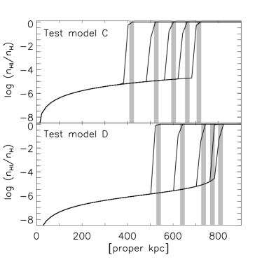
Figure 11: Comparison of test models C (upper panel) and D (lower panel) to the analytical solution for the size of a H $\rm\scriptstyle II\$region in a pure hydrogen medium of constant temperature and density. The solid lines show the numerical solution for the H $\rm\scriptstyle I\$fraction at $t/10^{7}\rm~{}yrs=[0.2,0.4,0.6,0.8,1.0]$ for model C and $t/10^{7}\rm~{}yrs=[0.05,0.1,0.2,0.3,1.0]$ for model D. The centre of the solid grey strips give the analytical solution with the width of the strips representing the cell size of the simulation.

We compare the results of test models C and D to the classical analytical solution, equation (3), in figure 11. The solid lines show the numerical solution for the H $\rm\scriptstyle I\$fraction at $t/10^{7}\rm~{}yrs=[0.2,0.4,0.6,0.8,1.0]$ for model C and $t/10^{7}\rm~{}yrs=[0.05,0.1,0.2,0.3,1.0]$ for model D. The solid grey strips give the analytical solution with a width equal to the cell size of the simulation, and hence the uncertainty in the numerical result. For this test we adopt a cell size of $\delta R=20\rm~{}kpc$, with $\epsilon=0.1$ for model C and $\epsilon=0.01$ for model D. The agreement between the numerical and analytical results is very good, which suggests that we are calculating the extent of the H $\rm\scriptstyle II\$regions correctly within our radiative transfer implementation. Note that by $t/10^{7}\rm~{}yrs=1.0$ model D has reached its Strömgren radius.

Appendix D A simple model for self-shielded regions

After the low density gas in the IGM has been reionized, dense, self-shielded clumps (SSCs) are thought to set the mean free path for ionizing photons (e.g. Miralda-Escudé et al. 2000, hereinafter MHR00, Miralda-Escudé 2003). We adopt a simple model to include these SSCs within our simulations. As noted by Furlanetto & Oh (2005), one may approximate the density at which hydrogen in a dense clump becomes self-shielded. For a clump of normalised density $\Delta=\rho_{\rm b}/\bar{\rho}_{\rm b}$ in ionization equilibrium with the UV background, its column density is approximately (Schaye 2001),

$$N_{\rm HI}=4.5\times 10^{14}\frac{\Delta^{3/2}}{\Gamma_{-12}^{\rm b}}\left(\frac{T}{10^{4}\rm~{}K}\right)^{0.2}\left(\frac{1+z}{7}\right)^{9/2}\rm~{}cm^{-2},$$ (30)

where $\Gamma_{-12}^{\rm b}=\Gamma_{\rm HI}^{\rm b}/10^{-12}\rm~{}s^{-1}$ is the normalised metagalactic hydrogen ionization rate and $T$ is the gas temperature. The clump will become optically thick to ionizing radiation once $N_{\rm HI}\geq 1/\sigma_{\rm HI}=1.6\times 10^{17}\rm~{}cm^{-2}$. Adopting this value for $N_{\rm HI}$ and rearranging yields the expected normalised density threshold for a SSC immersed in the metagalactic radiation field

$$\Delta_{\rm SSC}\simeq 49.5\left(\frac{T}{10^{4}\rm~{}K}\right)^{0.13}\left(\frac{1+z}{7}\right)^{-3}\left(\Gamma_{-12}^{\rm b}\right)^{2/3}.$$ (31)

For UV background models $6$, $9$ and $10$, which produce IGM neutral fractions consistent with the observational data of Fan et al. (2006b), this implies $\Delta_{\rm SSC}=[4.1,21.2,37.5]$ at $z=[6.25,6,5.75]$. Ideally, we would implement this self-shielding for $\Delta\geq\Delta_{\rm SSC}$ within our radiative transfer simulations in the same way as MHR00, by assuming all regions with $\Delta\geq\Delta_{\rm SSC}$ remain neutral while still optically thick to ionizing radiation. However, although we have shown that the resolution of our hydrodynamical simulation should be sufficient for correctly modelling the propagation of ionizing radiation, it still does not quite reach the required mass resolution to reproduce the correct number of clumps with $\Delta\geq\Delta_{\rm SSC}$. MHR00 overcome this problem by using an IGM density distribution drawn from a hydrodynamical simulation, with the addition of a power-law high density tail to account for the lack of high density clumps. The mean free path for ionizing photons in their model is given by

$$\lambda_{\rm mfp}=\frac{60}{H(z)}\left[1-F_{\rm V}(\Delta<\Delta_{\rm SSC})\right]^{-2/3}\rm~{}Mpc,$$ (32)

where $H(z)$ is the Hubble parameter and $F_{\rm V}(\Delta<\Delta_{\rm SSC})$ is the fraction of the IGM volume with $\Delta<\Delta_{\rm SSC}$, computed from the volume weighted density distribution corrected for high densities. Assuming $\lambda_{\rm mfp}$ is similar to the mean distance between SSCs, which is expected to be a reasonable approximation (Furlanetto & Oh 2005), the number of SSCs per unit redshift with $\Delta\geq[4.1,21.2,37.5]$ at $z=[6.25,6,5.75]$ using the MHR00 model is

$$\frac{dN_{\rm SSC}}{dz}\simeq\frac{1}{\lambda_{\rm mfp}}\frac{c}{H(z)(1+z)}=[52.5,9.0,5.1].$$ (33)

In comparison, the number of clumps per unit redshift with $\Delta\geq[4.1,21.2,37.5]$ at $z=[6.25,6,5.75]$ within our $400^{3}$ simulation volume is around a factor of two less than this. Therefore, when setting all clumps with $\Delta\geq\Delta_{\rm SSC}$ to be neutral within our simulations using UVB models 6, 9 and 10, we underpredict the mean free path for ionizing photons by about a factor of two. To compensate for this, we lower the density threshold at which a clump becomes self-shielded, thus reproducing the required number of SSCs per unit redshift given by the MHR00 model, as listed in equation (33). The relevant density thresholds in our $400^{3}$ simulation which reproduce the required number of SSCs per unit redshift are $\Delta_{\rm SSC}=[2.7,10.0,20.0]$ at $z=[6.25,6,5.75]$. Thus, our simulations using $\Delta_{\rm SSC}=[2.7,10.0,20.0]$ and UV background models 6, 9 and 10 at $z=[6.25,6,5.75]$ should be equivalent to using $\Delta_{\rm SSC}=[4.1,21.2,37.5]$ with $\lambda_{\rm mfp}=[1.09,6.99,12.80]\rm~{}Mpc$ and $\Gamma_{-12}^{\rm b}=[0.028,0.280,0.560]$. Assuming ionization equilibrium at $\Delta=1$ and $T=2\times 10^{4}\rm~{}K$, these ionization rates correspond to $f_{\rm HI}=[7.3\times 10^{-4},7.3\times 10^{-5},3.6\times 10^{-5}]$. However, we note that simulations incorporating radiative transfer which correctly resolve the number density of SSCs are needed to fully address their effect on observed near-zone sizes.

References

- Abel et al. (1997) Abel T., Anninos P., Zhang Y., Norman M. L., 1997, New Astron., 2, 181
- Abel & Haehnelt (1999) Abel T., Haehnelt M. G., 1999, ApJ, 520, L13
- Abel et al. (1999) Abel T., Norman M. L., Madau P., 1999, ApJ, 523, 66
- Anninos et al. (1997) Anninos P., Zhang Y., Abel T., Norman M. L., 1997, New Astron., 2, 209
- Bajtlik et al. (1988) Bajtlik S., Duncan R. C., Ostriker J. P., 1988, ApJ, 327, 570
- Barkana & Loeb (2004) Barkana R., Loeb A., 2004, ApJ, 601, 64
- Becker et al. (2006) Becker G. D., Rauch M., Sargent W. L. W., 2006, ApJ submitted, astro-ph/0607633
- Becker et al. (2005) Becker G. D., Sargent W. L. W., Rauch M., 2005, in Williams P., Shu C.-G., Menard B., eds, IAU Colloq. 199: Probing Galaxies through Quasar Absorption Lines, p.357
- Becker et al. (2006b) Becker G. D., Sargent W. L. W., Rauch M., Simcoe R. A., 2006b, ApJ, 640, 69
- Becker et al. (2001) Becker R. H. et al., 2001, AJ, 122, 2850
- Bolton et al. (2004) Bolton J., Meiksin A., White M., 2004, MNRAS, 348, L43
- Bolton et al. (2005) Bolton J. S., Haehnelt M. G., Viel M., Springel V., 2005, MNRAS, 357, 1178
- Cen (1992) Cen R., 1992, ApJS, 78, 341
- Cen & Haiman (2000) Cen R., Haiman Z., 2000, ApJ, 542, L75
- Cen & McDonald (2002) Cen R., McDonald P., 2002, ApJ, 570, 457
- Ciardi & Loeb (2000) Ciardi B., Loeb A., 2000, ApJ, 540, 687
- Djorgovski et al. (2001) Djorgovski S. G., Castro S., Stern D., Mahabal A. A., 2001, ApJ, 560, L5
- Donahue & Shull (1987) Donahue M., Shull J. M., 1987, ApJ, 323, L13
- Eisenstein & Hu (1999) Eisenstein D. J., Hu W., 1999, ApJ, 511, 5
- Fan et al. (2006a) Fan X., Carilli C. L., Keating B., 2006a, ARA&A, 44, 415
- Fan et al. (2001) Fan X. et al., 2001, AJ, 122, 2833
- Fan et al. (2002) Fan X., Narayanan V. K., Strauss M. A., White R. L., Becker R. H., Pentericci L., Rix H.-W., 2002, AJ, 123, 1247
- Fan et al. (2006b) Fan X. et al., 2006b, AJ, 132, 117 (F06b)
- Fan et al. (2000) Fan X. et al., 2000, AJ, 120, 1167
- Furlanetto & Loeb (2003) Furlanetto S. R., Loeb A., 2003, ApJ, 588, 18
- Furlanetto & Oh (2005) Furlanetto S. R., Oh S. P., 2005, MNRAS, 363, 1031
- Gallerani et al. (2006) Gallerani S., Choudhury T. R., Ferrara A., 2006, MNRAS, 370, 1401
- Gnedin (2000) Gnedin N. Y., 2000, ApJ, 535, 530
- Gnedin (2004) Gnedin N. Y., 2004, ApJ, 610, 9
- Gnedin & Fan (2006) Gnedin N. Y., Fan X., 2006, ApJ, 648, 1
- Gunn & Peterson (1965) Gunn J. E., Peterson B. A., 1965, ApJ, 142, 1633
- Hjerting (1938) Hjerting F., 1938, ApJ, 88, 508
- Hopkins et al. (2005) Hopkins P. F., Hernquist L., Martini P., Cox T. J., Robertson B., Di Matteo T., Springel V., 2005, ApJ, 625, L71
- Hu et al. (2005) Hu E. M., Cowie L. L., Capak P., Kakazu Y., 2005, in Williams P., Shu C.-G., Menard B., eds, IAU Colloq. 199: Probing Galaxies through Quasar Absorption Lines, p.363
- Iliev et al. (2006a) Iliev I. T. et al., 2006a, MNRAS, 371, 1057
- Iliev et al. (2006b) Iliev I. T., Mellema G., Pen U.-L., Merz H., Shapiro P. R., Alvarez M. A., 2006b, MNRAS, 369, 1625
- Kashikawa et al. (2006) Kashikawa N. et al., 2006, ApJ, 648, 7
- Katz et al. (1996) Katz N., Weinberg D. H., Hernquist L., 1996, ApJS, 105, 19
- Kohler et al. (2005) Kohler K., Gnedin N. Y., Hamilton A. J. S., 2005, preprint, astro-ph/0511627
- Lidz et al. (2006) Lidz A., Oh S. P., Furlanetto S. R., 2006, ApJ, 639, L47
- Liu et al. (2006) Liu J., Bi H., Feng L.-L., Fang L.-Z., 2006, ApJ, 645, L1
- Madau et al. (1999) Madau P., Haardt F., Rees M. J., 1999, ApJ, 514, 648
- Madau et al. (1997) Madau P., Meiksin A., Rees M. J., 1997, ApJ, 475, 429
- Madau & Rees (2000) Madau P., Rees M. J., 2000, ApJ, 542, L69
- Malhotra & Rhoads (2004) Malhotra S., Rhoads J. E., 2004, ApJ, 617, L5
- Martini (2004) Martini P., 2004, in Ho L. C., ed., Coevolution of Black Holes and Galaxies QSO Lifetimes, p.169
- Mellema et al. (2006) Mellema G., Iliev I. T., Alvarez M. A., Shapiro P. R., 2006, New Astron., 11, 374
- Mesinger & Haiman (2004) Mesinger A., Haiman Z., 2004, ApJ, 611, L69
- Mesinger et al. (2004) Mesinger A., Haiman Z., Cen R., 2004, ApJ, 613, 23
- Miralda-Escudé et al. (2000) Miralda-Escudé J., Haehnelt M., Rees M. J., 2000, ApJ, 530, 1 (MHR00)
- Miralda-Escudé (1998) Miralda-Escudé J., 1998, ApJ, 501, 15
- Miralda-Escudé & Rees (1998) Miralda-Escudé J., Rees M. J., 1998, ApJ, 497, 21
- Miralda-Escudé (2003) Miralda-Escudé J., 2003, ApJ, 597, 66
- Mo & White (2002) Mo H. J., White S. D. M., 2002, MNRAS, 336, 112
- Oh (2002) Oh S. P., 2002, MNRAS, 336, 1021
- Oh & Furlanetto (2005) Oh S. P., Furlanetto S. R., 2005, ApJ, 620, L9
- Olive & Skillman (2004) Olive K. A., Skillman E. D., 2004, ApJ, 617, 29
- Osterbrock (1989) Osterbrock, D.E., 1989, Astrophysics of Gaseous Nebulae and Active Galactic Nuclei, University Science Books, Mill Valley, CA
- Page et al. (2006) Page L. et al., 2006, ApJ submitted, astro-ph/0603450
- Paschos & Norman (2005) Paschos P., Norman M. L., 2005, ApJ, 631, 59
- Peebles (1971) Peebles, P.J.E., 1971, Physical Cosmology, Princeton University Press, Princeton, NJ
- Peebles (1993) Peebles, P.J.E., 1993, Principles of Physical Cosmology, Princeton University Press, Princeton, NJ
- Pentericci et al. (2002) Pentericci L. et al., 2002, AJ, 123, 2151
- Schaye (2001) Schaye J., 2001, ApJ, 559, 507
- Scott & Rees (1990) Scott D., Rees M. J., 1990, MNRAS, 247, 510
- Seljak et al. (2006) Seljak U., Slosar A., McDonald P., 2006, preprint, astro-ph/0604335
- Shapiro & Giroux (1987) Shapiro P. R., Giroux M. L., 1987, ApJ, 321, L107
- Shapiro et al. (2006) Shapiro P. R., Iliev I. T., Alvarez M. A., Scannapieco E., 2006, ApJ, 648, 922
- Shapiro et al. (2004) Shapiro P. R., Iliev I. T., Raga A. C., 2004, MNRAS, 348, 753
- Shaver et al. (1999) Shaver P. A., Windhorst R. A., Madau P., de Bruyn A. G., 1999, A&A, 345, 380
- Songaila (2004) Songaila A., 2004, AJ, 127, 2598
- Songaila & Cowie (2002) Songaila A., Cowie L. L., 2002, AJ, 123, 2183
- Spergel et al. (2006) Spergel D. N. et al., 2006, ApJ submitted, astro-ph/0603449
- Spitzer (1978) Spitzer, L., 1978, Physical Processes in the Interstellar Medium, Wiley Interscience, New York
- Springel (2005) Springel V., 2005, MNRAS, 364, 1105
- Springel & Hernquist (2003) Springel V., Hernquist L., 2003, MNRAS, 339, 289
- Strömgren (1939) Strömgren B., 1939, ApJ, 89, 526
- Theuns et al. (1998) Theuns T., Leonard A., Efstathiou G., Pearce F. R., Thomas P. A., 1998, MNRAS, 301, 478
- Tittley & Meiksin (2006) Tittley E. R., Meiksin A., 2006, MNRAS submitted, astro-ph/0605317
- Totani et al. (2006) Totani T. et al., 2006, PASJ, 58, 485
- Tozzi et al. (2000) Tozzi P., Madau P., Meiksin A., Rees M. J., 2000, ApJ, 528, 597
- Viel et al. (2006) Viel M., Haehnelt M. G., Lewis A., 2006, MNRAS, 370, L51
- Volonteri & Rees (2006) Volonteri M., Rees M. J., 2006, ApJ in press, astro-ph/0607093
- Walter et al. (2004) Walter F., Carilli C., Bertoldi F., Menten K., Cox P., Lo K. Y., Fan X., Strauss, M. A., 2004, ApJ, 615, L17
- White et al. (2003) White R. L., Becker R. H., Fan X., Strauss M. A., 2003, AJ, 126, 1
- White et al. (2005) White R. L., Becker R. H., Fan X., Strauss M. A., 2005, AJ, 129, 2102
- Wyithe & Loeb (2004) Wyithe J. S. B., Loeb A., 2004, Nature, 427, 815
- Wyithe et al. (2005) Wyithe J. S. B., Loeb A., Carilli C., 2005, ApJ, 628, 575
- Wyithe & Loeb (2006) Wyithe J. S. B., Loeb A., 2006, ApJ, 646, 696
- Yu (2005) Yu Q., 2005, ApJ, 623, 683
- Yu & Lu (2005) Yu Q., Lu Y., 2005, ApJ, 620, 31