Neutrinos from galactic sources of cosmic rays

with known $\gamma$-ray spectra

Francesco Vissani

INFN, Laboratori Nazionali del Gran Sasso, Assergi (AQ)

We describe a simple procedure to estimate the high-energy neutrino flux from the observed $\gamma$-ray spectra of galactic cosmic ray sources that are transparent to their gamma radiation. We evaluate in this way the neutrino flux from the supernova remnant RX J1713.7-3946, whose very high-energy $\gamma$-ray spectrum (assumed to be of hadronic origin) is not a power law distribution according to H.E.S.S. observations. The corresponding muon signal in neutrino telescopes is found to be about 5 events per km² per year in an ideal detector. PACS: Neutrinos from CR 98.70.Sa; Observations of $\gamma$-rays 95.85.Pw; SNR in Milky Way 98.38.Mz.

1 Context and motivations

The recent observations of $\gamma$-rays above TeV by H.E.S.S. are of great interest [1, 2]. They will certainly help in answering the old question of the origin of the cosmic rays till the knee [3, 4, 5, 6, 7] and at the same time they could provide us a reliable guidance for what we should expect in neutrino telescopes, at least for certain sources.

This is evident for the main candidate sources of galactic cosmic rays, supernova remnants (SNR) [8, 9]. The huge kinetic energy of the gas of the SNR could be effectively converted into cosmic rays by diffusive shock acceleration [10], producing enough cosmic rays to compensate the losses from the Milky Way. When the SNR is surrounded by matter that can act as a target for cosmic rays, we would have a point source of very high-energy (VHE) gamma radiation, which seems in agreement with certain observations. Since we expect that the matter around SNR is not too dense anyway, the $\gamma$-rays are not significantly absorbed, and there is a rather direct relation between VHE $\gamma$-rays and neutrinos.

More in general, we think that it is important to take advantage of the detailed observations of $\gamma$-rays whenever they exist in order to formulate definite expectations for neutrino telescopes. This is certainly true after the most recent H.E.S.S. observations, that are beginning to find VHE $\gamma$-ray spectra that deviate from power law distributions above 10 TeV or so [2].

Our recipe to calculate the neutrino fluxes is described in Sect. 2 and the application to the SNR RX J1713.7-3946 is in Sect. 3. In essence, these results are a straightforward application of standard techniques [11] (and we follow as much as possible the conventions of [4] to emphasise this fact) but we hope that they are useful in the present moment, when the high-energy gamma astronomy is flourishing and the neutrino telescopes are finally becoming a reality.

2 Deriving the neutrino flux from the $\gamma$-ray flux

Let us assume that the VHE $\gamma$-ray flux $F_{\gamma}$ observed from a certain source is of hadronic origin and that it is not significantly absorbed–the source is $\gamma$-transparent. From the well-known relation $F_{\gamma}(E)=\int_{E}^{\infty}dE^{\prime}\ 2\ F_{\pi^{0}}(E^{\prime})/E^{\prime}$ valid for high-energy $\gamma$-rays we find:

$$F_{\pi^{0}}(E)=-\frac{E}{2}\ \frac{dF_{\gamma}}{dE}$$ (1)

that implies that the $\gamma$-ray flux has to be strictly decreasing. This equation, together with the approximate isospin-invariant distribution of pions:

$$F_{\pi}\equiv F_{\pi^{0}}\approx F_{\pi^{+}}\approx F_{\pi^{-}}$$ (2)

permits us to predict the flux of neutrinos using the observed $\gamma$-ray flux. It is important to note that the charge asymmetry has a small or negligible impact on the observable $\nu_{\mu}$ flux, compare [14, 15]. The $\nu_{\mu}$ flux from the decay $\pi^{+}\to\mu^{+}\nu_{\mu}$ is:

$$F_{\nu_{\mu}}(E)=\frac{F_{\gamma}(E/(1-r))}{2(1-r)}$$ (3)

where $r=(m_{\mu}/m_{\pi})^{2}$. The neutrinos from muon decay $\mu^{+}\to\bar{\nu}_{\mu}\nu_{e}e^{+}$ have a more implicit expression:

$$F_{\nu}(E_{\nu})=\int^{1}_{0}\frac{dy}{y}\ F_{\mu}(E_{\mu})\ (g_{0}(y)-\bar{P_{\mu}}(E_{\mu})\ g_{1}(y))$$ (4)

where $E_{\mu}=E_{\nu}/y$ and $g_{i}$ are known polynomials: $g_{0}=5/3-3y^{2}+4/3y^{3}$ and $g_{1}=1/3-3y^{2}+8/3y^{3}$ when $\nu=\bar{\nu}_{\mu}$, while $g_{0}=2-6y^{2}+4y^{3}$ and $g_{1}=-2+12y-18y^{2}+8y^{3}$ when $\nu={\nu}_{e}$ [11]. The muon flux (from $\pi^{+}$) that appears in previous formula is:

$$F_{\mu}(E)=\frac{F_{\gamma}(E)-F_{\gamma}(E/r)}{2(1-r)}$$ (5)

while the muon polarisation averaged over the pion distribution is given by:

$$\bar{P_{\mu}}(E)\times F_{\mu}(E)=-\frac{F_{\gamma}(E)+F_{\gamma}(E/r)}{2(1-r)}+\frac{r}{(1-r)^{2}}\int_{E}^{E/r}\!\!F_{\gamma}(E^{\prime})\ \frac{dE^{\prime}}{E}$$ (6)

It is easy to check that in the special case of power law distributions these equations reproduce the results of Sect. 7.1 of [4] (e.g., eq. 7.14 there).

We include the contribution to $\gamma$ flux from $\eta\to\gamma\gamma$ (resp., the contribution to $\nu$ flux from the leptonic $K^{\pm}$ decay) in the simplest conceivable approximation: namely, we declare that the relevant flux of eta mesons (resp., the one of charged kaons) is proportional to the one of the neutral pions (resp., of the charged pions) with a fixed coefficient $f_{\eta}=10$ % (resp. $f_{K}=25$ % $\times 0.635$). Thus: (1) all formulae above should be multiplied by $1/(1+f_{\eta})$, and then (2) we add a neutrino contribution that has the same form as the one from charged pions, but replacing $r=(m_{\mu}/m_{K})^{2}$ and including the multiplicative factor $f_{K}$.

Finally, we incorporate 3 neutrino oscillations replacing:

$$F_{\nu_{\mu}}\to F_{\nu_{\mu}}\ P_{\mu\mu}+F_{\nu_{e}}\ P_{e\mu}$$ (7)

and the same for antineutrinos. The numerical values of the oscillation probabilities are $P_{\mu\mu}=0.39\pm 0.05$ and $P_{e\mu}=0.22\mp 0.05$ where the quoted errors, approximately equal and opposite, are mostly (0.04) due to the spread of $\theta_{23}$ around maximal mixing and partly (0.02) to the spread of $\theta_{13}$ around zero; the effect of the uncertainty in $\theta_{12}$ is smaller. See [14] for more discussion, [16] for a resumé of neutrino data and analysis, and [17] for further references.

We note in passing a stricter condition on the behaviour of the flux of VHE secondaries with the energy. Consider the connection with the primary cosmic rays $F_{\pi}(E)\propto\int_{E}^{\infty}dE^{\prime}F_{p}(E^{\prime})k(E/E^{\prime})/E$, that we assume for simplicity to be protons. When we go from $E=E_{1}$ to $E=E_{2}$ with $E_{2}>E_{1}$, the integral decreases because 1) the lower limit increases; 2) the scaling distribution $k$ in the integrand is a decreasing function; 3) there is an explicit factor $1/E$. Thus, also $f_{\pi}(E)\equiv EF_{\pi}(E)$ decreases. The same can be said of the function $f_{\gamma}(E)=EF_{\gamma}(E)$, since $f_{\gamma}(E)=2\int_{0}^{1}f_{\pi}(E/z)dz$; in other words the flux of hadronic $\gamma$-rays decreases at least as $1/E$ at high energies.

3 Application: neutrinos from RX J1713.7-3946

We apply the formalism of the previous section to obtain the expected neutrino flux from RX J1713.7-3946 on the basis of H.E.S.S. observations [2]. We use 2 parameterisations of the $\gamma$-ray flux that describe well the observations [2]:

$$F_{\gamma}(E)=\left\{\begin{array}[]{ll}20.4\ E^{-1.98}\ \exp(-E/12)&[\mbox{exponential cutoff}]\\[4.30554pt] 20.1\ E^{-2.06}\ [1+(E/6.7)^{2.5}]^{-0.496}&[\mbox{broken power law}]\end{array}\right.$$ (8)

where the units are TeV for the energy $E$ and $10^{-12}/(\mbox{TeV cm${}^{2}$ s})$ for the flux $F_{\gamma}(E)$. We do not use the third parametrization proposed in [2], $F_{\gamma}\propto E^{-2.08-0.3\log E}$, namely the distribution with energy dependent photon index: in fact, this cannot result from $\pi^{0}$s, since this is just a Gaussian in the logarithmic variable $\log E$, that increases rather than decreasing before 40 GeV. Note that a relatively low cutoff implied by H.E.S.S. observations is consistent with the present theoretical expectations [18] (however, rather different models of the same object are also discussed [19]). The result for muon neutrinos according to formulae 3, 4 and 7 is presented in figure 1 and table 1; in our approximation, the flux of antineutrinos is the same.

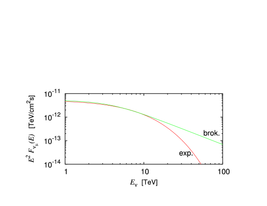
Figure 1: Expected $\nu_{\mu}$ fluxes corresponding to the two $\gamma$-ray spectra of eq. 8.

We can estimate the number of through-going events in a neutrino telescope with $E_{th}=50$ GeV, $\phi=42^{\circ}50^{\prime}$ (ANTARES location) following [14]. Considering neutrinos with energies below $E_{\nu,\rm max}=300$ TeV (that is not a significant limitation), we find:

$$N_{\mu+\bar{\mu}}=\left\{\begin{array}[]{ll}\mbox{4.8 per km${}^{2}$ per year}&\mbox{ [exponential cutoff] }\\ \mbox{5.4 per km${}^{2}$ per year}&\mbox{ [broken power law]}\end{array}\right.$$ (9)

that can be compared with $N_{\mu+\bar{\mu}}=8.8$ of [14], obtained assuming a power law distribution. Thus, the new H.E.S.S. data suggest a signal about 8 times weaker than given in [20] (resp., 2 times weaker than in [14]) that adopted a power law distribution extrapolated from the first observations of CANGAROO (resp., of H.E.S.S.).

One can gain something if some events above the horizon are accepted; e.g., with $5^{\circ}$ more, one can go from a fraction of time useful for observation of 78 % (used for the numbers quoted in eq. 9) to 88 %. This is similar to effects here neglected, e.g., other contributions of $\eta$ and $K$ meson decays or the deviations of $\theta_{23}$ from maximal mixing, and should be comparable with the error of the method of calculation we proposed. The effect of finite detection efficiency for realistic detector configurations instead should be more important (comparable with the effect of the deviation from a power law distribution discussed here) for the events are not expected to be particularly energetic: the distribution of parent neutrino energies has a median of 3 TeV for both distributions of eq. 8.

Table 1: $1^{st}$ line: selected values of neutrino energy. $2^{st}$ line: sum of the yields of muons and antimuons (including Earth absorption), times the reference area $A=1$ km² and observation time $T=1$ year. $3^{nd}$ and $4^{rd}$ line: the $F_{\nu_{\mu}}/F_{\gamma}$ ratio for the $\gamma$-ray fluxes of eq. 8, which varies significantly with the energy.

$E$ [TeV]	.1	.3	1	3	10	30	100	300
$AT(Y_{\mu}\!+\!Y_{\bar{\mu}})$ [cm2 s]	$1.0\mbox{\tt\scriptsize E}{9}$	$2.3\mbox{\tt\scriptsize E}{10}$	$2.8\mbox{\tt\scriptsize E}{11}$	$1.9\mbox{\tt\scriptsize E}{12}$	$1.1\mbox{\tt\scriptsize E}{13}$	$3.5\mbox{\tt\scriptsize E}{13}$	$9.2\mbox{\tt\scriptsize E}{12}$	$1.6\mbox{\tt\scriptsize E}{14}$
$F_{\nu_{\mu}}/F_{\gamma}$, exp. cutoff	.26	.26	.25	.21	.14	.06	.02	.01
$F_{\nu_{\mu}}/F_{\gamma}$, brok. power	.25	.25	.25	.21	.14	.13	.13	.13

4 Summary and discussion

In summary, we presented a simple procedure to convert the observations of high-energy $\gamma$-rays into expectations for high-energy neutrinos, assuming that the source is gamma-transparent and that the flux of VHE $\gamma$-ray is due to cosmic ray interactions (=it is of hadronic origin). The latter hypothesis shows that our flux should be thought as an upper bound for gamma-transparent sources. As an application, we calculated the neutrino flux from RX J1713.7-3946 expected on the basis of new H.E.S.S. results and found that the expected number of events decreases by $40-50$ % and that the signal consists of relatively low energy events.

In the future, it will be interesting to repeat the same steps for other intense sources of VHE $\gamma$-rays, e.g., Vela Jr (RX J0852.0-4652), that is almost continuously visible from ANTARES (95 % of time). In the region $E\leq 10$ TeV [1] the spectrum is described by $F_{\gamma}=21\ E^{-2.1}$ (same units as in eq. 8). Suppose that the future observations will demonstrate a milder exponential cutoff, described by a multiplicative factor $\exp(-E/E_{\rm cut})$ with $E_{\rm cut}=50\ (150)$ TeV. In this case we would find $N_{\mu+\bar{\mu}}=10$ (14) events per km² per year with a median neutrino energy of 5.5 (8.5) TeV (if, again, we assume that all $\gamma$-rays are hadronic). If instead RX J1713.7-3946 should turn out to represent a typical SNR in a typical stage, it will be important to understand the cosmic rays from a few hundred TeV till the knee, e.g., considering other galactic point sources of cosmic rays and/or further phases of cosmic ray acceleration.

These results emphasise even further the importance to obtain $\gamma$-ray observations in the region from 10 to 100 TeV and to understand well the experimental background coming from atmospheric neutrinos.

We gratefully thank F. Aharonian, V. Berezinsky, P.L. Ghia, D. Grasso and especially P. Lipari for useful discussions and M.L. Costantini for help.

Note added

After this work was submitted for publication and when it was presented at Vulcano 2006 conference (May 2006), a number of interesting new works appeared: [21] where the background and possible strategies for neutrino search are quantitatively discussed; [22], where a detailed parameterizations of neutrino and gamma yields is offered; [23], where neutrinos events from Vela Jr are estimated (though, without describing the details of the calculation) using a fixed $\nu/\gamma$ conversion coefficient $=1/2$.

References

- [1] See e.g., H.E.S.S. Collaboration, Astron. Astrophys. 437 (2005) L7, ibid. 95, ibid. 135; Astron. Astrophys. 439 (2005) 1013; Astrophys.J.636 (2006) 777
- [2] F. Aharonian et al. [The HESS Collaboration], A detailed spectral and morphological study of the gamma-ray supernova remnant RX J1713.7-3946 with HESS, Astron. Astrophys. 449 (2006) 223
- [3] V.S Berezinsky, S.V. Bulanov, V.A. Dogiel, V.L. Ginzburg (ed.), V.S. Ptuskin, Astrophysics of cosmic rays, (1990, Russian edition 1984) North Holland
- [4] T.K Gaisser, Cosmic rays and particle physics (1990) Cambridge Univ. Pr.
- [5] T. Stanev, High energy cosmic rays (2003) Springer
- [6] F. Aharonian, Very high energy cosmic radiation (2004) World Scientific
- [7] V.S. Ptuskin, Origin of galactic cosmic rays: sources, acceleration, and propagation, Rapporteur talk at 29th ICRC (2005) 10, 317
- [8] W. Baade, F. Zwicky, Phys. Rev. 45 (1934) 138
- [9] V.L. Ginzburg, S.I. Syrovatsky, Origin of Cosmic Rays (1964) Moscow
- [10] For reviews see L.O’C. Drury et al., Space Sci. Rev. 99 (2001) 329; M.A. Malkov, L.O’C. Drury, Rep. Prog. in Physics 64 (2003) 429; A.M. Hillas, J. Phys. G, Nucl. Part. Phys. 31 (2005) R95
- [11] P. Lipari as quoted in the caption of tab. 7.2 of [4]. See also L.V. Volkova, Proceedings of Erice 1988 Cosmic -rays, neutrinos, and related astrophysics page 139 and S.M. Barr, T.K. Gaisser, P. Lipari and S. Tilav, Phys. Lett. B214 (1988) 147
- [12] C. Distefano, D. Guetta, E. Waxman and A. Levinson, Astrophys. J. 575 (2002) 378. See W. Bednarek, G.F. Burgio and T. Montaruli, New Astron. Rev. 49 (2005) 1 for a review of possible galactic neutrino sources
- [13] H.E.S.S. Collaboration, Nature 440 (2006) 1018
- [14] M.L. Costantini and F. Vissani, Astropart. Phys. 23 (2005) 477
- [15] V. Cavasinni, D. Grasso and L. Maccione, astro-ph/0604004
- [16] A. Strumia and F. Vissani, Nucl. Phys. B 726 (2005) 294 and hep-ph/0606054; G.L. Fogli, E. Lisi, A. Marrone and A. Palazzo, hep-ph/0506083
- [17] S.M. Bilenky and B. Pontecorvo, Phys. Rept. 41 (1978) 225; J. Learned and S. Pakvasa, Astroparticle Phys. 3 (1995) 267; R.M. Crocker, F. Melia, R.R. Volkas, Astroph.J. Suppl. 130 (2000) 339; H. Athar, M. Jezabek and O. Yasuda, Phys. Rev. D 62 (2000) 103007; R.M. Crocker, F. Melia, R.R. Volkas, Astroph.J. Suppl. 141 (2002) 147; J.F. Beacom, N.F. Bell, D. Hooper, S. Pakvasa, T.J. Weiler, Phys.Rev. D 68 (2003) 0930005
- [18] E.G. Berezhko and H.J. Volk, astro-ph/0602177
- [19] M.A. Malkov, P.H. Diamond and R.Z. Sagdeev, Astrophys. J. 624 (2005) L37
- [20] J. Alvarez-Muniz and F. Halzen, Astrophys. J. 576 (2002) L33
- [21] P. Lipari, astro-ph/0605535
- [22] S. R. Kelner, F. A. Aharonian and V. V. Bugayov, astro-ph/0606058
- [23] U.F. Katz, astro-ph/0606068