Contributed paper at the All-Russian Astronomical conference ”Close Binary Stars in Modern Astrophysics (MARTYNOV-2006)” held in Moscow, Russia May 22 - 24, 2006

We carried out numerical experiments on the evaluation of the possibilities of obtaining the information about brightness distributions for the components of eclipsing variables from the data of high-precision photometry expected for planned satellites COROT and Kepler. We examined a simple model of the eclipsing binary with the spherical components on circular orbits and the linear law of the limb darkening. The solutions of light curves have been obtained as by fitting of the nonlinear model, into the number of parameters of which included the limb darkening coefficients, so also by the solution of the ill-posed inverse problem of restoration of brightness distributions across the disks of stars without rigid model constraints on the form of these functions. The obtained estimations show that if the observational accuracy amounts to $10^{-4}$ then the limb darkening coefficients can be found with the relative error approximately $0.01$ . The brightness distributions across the disks of components can be restored also nearly with the same accuracy.

Keywords: stars; eclipsing variables; brightness distributions

Corresponding author. E-mail: BogdanovMB@info.sgu.ru

1. Introduction

A study of eclipsing variable stars is at present the basic information source about sizes of stars and brightness distributions across their disks. Information about brightness distributions is especially important, since it allows to test the models of the stellar atmospheres independent of spectral analysis data. The analysis of the light curve of eclipsing binary is the classical problem of astrophysics. The methods of solution of this problem are detailed and connected with the names of the noted researchers: H.N.Russell, D.Ya.Martynov, V.P.Tsesevich, J.E.Merrill, Z.Kopal, etc.

At present there are two basic approaches to the solution of the problem: the fitting of the nonlinear model with known laws of the limb darkening for components of the eclipsing variable and the solution of the ill-posed inverse problem of the restoration of brightness distributions across the disks of stars. However, the precision of a ground-based photometry ( the relative error of flux measurements, $\epsilon>10^{-3}$ ) substantially limits the accuracy of the obtained results.

The planned launches of the special satellites COROT and Kepler make it possible to expect a considerable increase in the precision of photometry of bright objects ( up to $\epsilon=10^{-5}$ ). Under these conditions new possibilities for the solution of the classical problem of investigating the eclipsing variable stars are opened [1].

The purpose of our paper is estimation of the possibilities of the determination of geometric parameters and brightness distributions for the components of eclipsing variables from the data of high-precision photometry both the model fitting method and the method of restoration of brightness distributions.

2. The model light curve

It is known that in the case of spherical components with a linear law of the limb darkening the problem of calculating of a light curve for an eclipsing variable has the exact solution, whose error is determined by the precision of the numerical estimation of one-dimensional definite integrals. Therefore for further analysis we chose the simple model of an eclipsing variable with the following parameters: the angle of orbital inclination, $i=89^{o}.0$; the radius of the first component in units of the orbital radius, $r_{1}=0.30$; the luminosity of the first component, $L_{1}=0.30$; the limb darkening coefficient of the first component, $x_{1}=0.50$; the radius of the second component, $r_{2}=0.20$; the luminosity of the second component, $L_{2}=0.70$; the limb darkening coefficient of the second component, $x_{2}=0.30$; The luminosities of the components are connected by the equation: $L_{1}+L_{2}=1$ .

It is known that the light losses in minima $(1-l)_{i}$ are described by the phase functions

$$(1-l)_{i}=\alpha^{i}(p,k)(1-l_{A}),$$

where $(1-l_{A})$ - the light loss at the moment of the internal contact of the disks, $k=r_{2}/r_{1}$, $\Delta=r_{1}(1+kp)$, and $\Delta$ - distance between centers of the stellar disks in units of the orbital radius. These phase functions, for one’s part, can be expressed via main phases for occultations $\alpha^{\prime}(p,k)$ and transits $\alpha^{\prime\prime}(p,k)$ [2]. The last two main phases are estimated numerically via calculations of one-dimensional definite integrals which depend on parameters $p$ and $k$ .

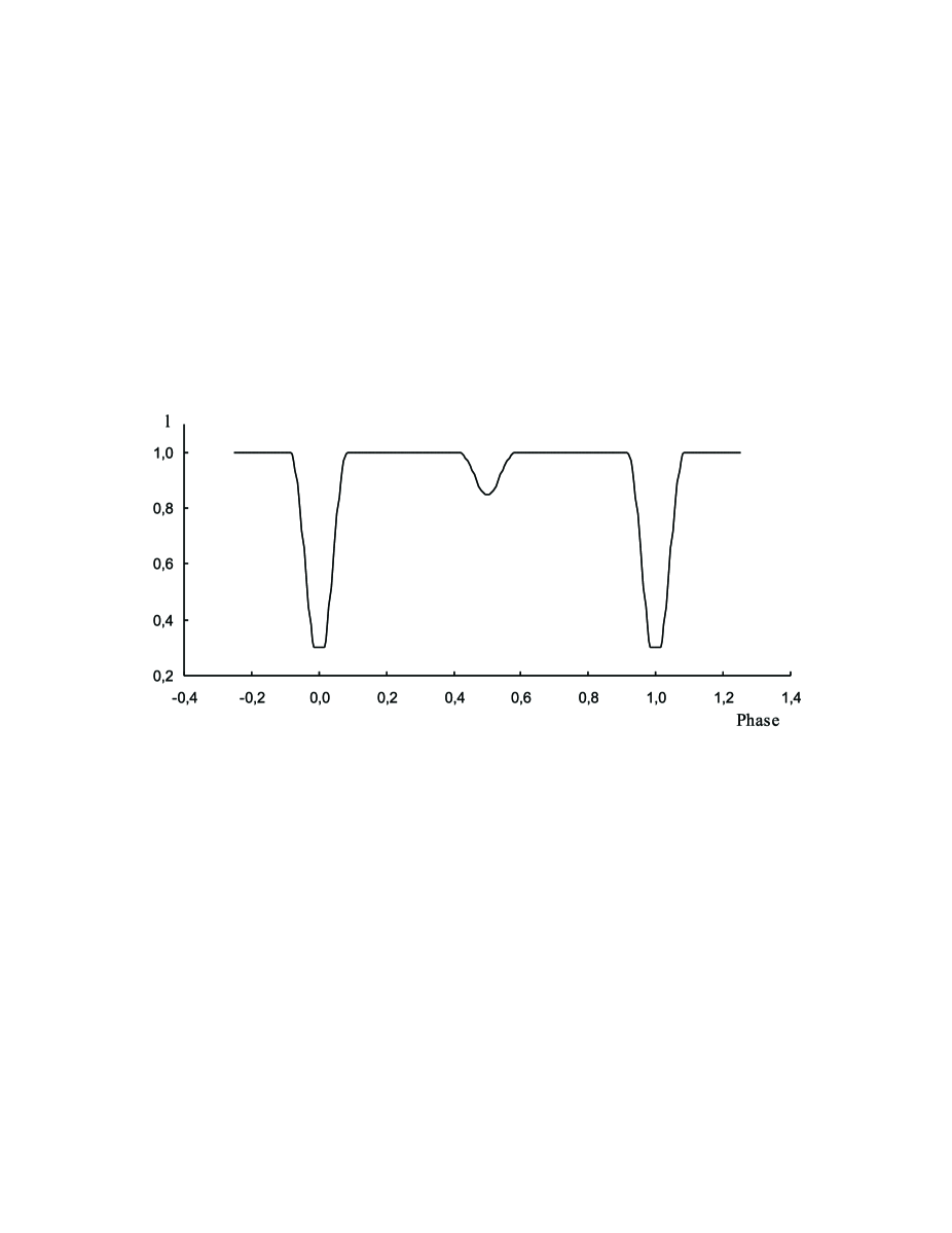
Figure 1: The calculated light curve for chosen model of the eclipsing variable.

We have calculated the definite integrals of phase functions by application of the Gauss - Kronrod algorithm using the subroutine DQAGE from the SLATEC FORTRAN program library. The precision of calculation of the light curve $l(i,L_{1},r_{1},x_{1},L_{2},r_{2},x_{2},\theta)$, where $\theta$ - the light phase $(0\leq\theta\leq 1)$, was adopted to be $\epsilon=10^{-12}$. The calculated light curve for our model of the eclipsing variable is shown in figure 1. In the primary minimum occurs the total eclipse, in the secondary - the annular eclipse.

3. The model fitting

One of basic approaches to the analysis of the light curves of the eclipsing variables is the fitting of the nonlinear model with known laws of the limb darkening for its components. As the input data we took our model light curve, perturbed by the influence of random noise with the various values of $\epsilon$ . The dispersion of noise was assumed to be constant in the magnitude scale. The Gaussian pseudo-random numbers $\Delta l_{i}$ with zero mean and the standard deviation equal to unity are used for the generation of the noise. Thus, the samples of perturbed light curve can be written as $l^{o}_{i}=l^{c}_{i}(1+\epsilon\Delta l_{i})$ , where $l^{c}_{i}$ - the samples of the calculated model light curve.

In both primary and secondary minimum we considered $N=100$ equidistant samples of the perturbed light curve. The search for optimal values of the model parameters leads to the solution of nonlinear minimization problems. In case of the primary minimum

$$\sum_{j=1}^{N}[l^{o}(\theta_{j})-l^{c}(i,r_{1},r_{2},L_{2},x_{2},\theta_{j})]^{2}=min$$

and

$$\sum_{j=1}^{N}[l^{o}(\theta_{j})-l^{c}(i,r_{1},r_{2},L_{1},x_{1},\theta_{j})]^{2}=min$$

for the secondary minimum. We have used for solutions of these problems the DNLS1 subroutine also from the SLATEC library which minimizes the sum of squares of nonlinear functions by a modification of the Levenberg - Marquardt algorithm [3].

Light curve nonlinearly depends on a number of parameters. This non-linearity can leads to the presence of the local minima of residual. For checking this possibility we carried out a number of numerical experiments on the solution of the problems of minimization (2) and (3) with different initial values of the model parameters. In these experiments the initial values were differed from the precise values up to two times in the side of an increase or decrease. In all cases the solution well converged to precise and, thus, the local minima not were discovered.

We carried out the model fitting to perturbed light curves for three values of $\epsilon=10^{-5},10^{-4}$, and $10^{-3}$ . In each case where examined $100$ curves with different realizations of the random noise. The obtained average values of the model parameters and their standard deviations are given in tables 1 and 2. As can be seen from these tables, the geometric parameters and the limb darkening coefficients are evaluated very accurately from data of the high-precision photometry. As a whole, a standard deviation in the estimation of a model parameter linearly decreases with the decrease of the relative error of the registration of light curve. If the observational accuracy of the space photometry amounts to $10^{-4}$ ( by one order higher than precision of ground-based photometry ) then the limb darkening coefficients can be found with the relative error approximately $0.01$ .

4. The restoration of brightness distributions

An alternative approach to the analysis of the light curves of the eclipsing variables - the restoration of brightness distributions across the stellar disks without rigid model constraints on the form of these functions was developed by Cherepashchuk et al. [4]. Let $I(\xi)$  $(0\leq\xi\leq r_{1})$ and $I(\rho)$  $(0\leq\rho\leq r_{2})$ are the brightness distributions across the disks of first and second component respectively. It can be shown that the light loss in the first and the second minimum are described by integral equations

$$1-l_{1}(\Delta)=\int_{0}^{r_{1}}K_{1}(\xi,\Delta,r_{2})I(\xi)d\xi$$

$$1-l_{2}(\Delta)=\int_{0}^{r_{2}}K_{2}(\rho,\Delta,r_{1})I(\rho)d\rho$$

Expressions for the kernels of these integral equations can be found in paper Cherepashchuk et al. [4] and monograph Tsesevich et al. [2].

The equations (4) and (5) are the integral equations of Fredholm’s first kind. The solution of this integral equation is an ill-posed problem in Hadamard’s sense and requires utilization of a priori information about sought function. It is possible to assume that for majority stars with thin photospheres the brightness distributions are non-negative, monotonically non-increasing, convex upward functions. It is known that the sets of functions of these types are the compact sets. The search for the solution of an ill-posed problem on the compact set of functions gives the unique and stable result [5]. This a priori information is qualitative and imposes no rigid model constraints on the form of the brightness distribution. Nevertheless, this guarantees that the obtained brightness distributions will approach their exact values as the errors in the registration of the observed light curve approach zero with exception of the points of discontinuity of the functions [5,6]. The use of a large amount of a priori information about the possible form of the brightness distribution in accordance with the physics of phenomenon enables us to achieve a solution with a high degree of stability against the effects of random noise.

Thus, as the solution of our problem can be taken the non-negative, monotonically non-increasing, convex upward functions $I(\xi)$ and $I(\rho)$ that minimize the following functions of functions - the norms in the $L_{2}$ function space:

$$\Phi_{1}[I(\xi),r_{1},r_{2},i]=\parallel\int_{0}^{r_{1}}K_{1}(\xi,\Delta,r_{2})I(\xi)d\xi-[1-l_{1}(\Delta)]\parallel_{L_{2}}$$

$$\Phi_{2}[I(\rho),r_{1},r_{2},i]=\parallel\int_{0}^{r_{2}}K_{2}(\rho,\Delta,r_{1})I(\rho)d\rho-[1-l_{2}(\Delta)]\parallel_{L_{2}}$$

The problem of restoration of the brightness distributions depends also on three free parameters: $i,r_{1}$ and $r_{2}$ , whose values can be found by the minimization of the summary residual.

We carried out the numerical experiment on the restoration of brightness distributions from our perturbed model light curve for the value of $\epsilon=10^{-4}$ . The special estimations showed that the choice of the number of points $M=1001$ of an uniform grid along a radius with the integration for Simpson’s formula makes it possible to ensure an relative error in the calculation of integrals (4) and (5) below to $10^{-6}$ . These grids where used later on for the minimization of functions of functions. We minimized the summary residual for both minima

$$\Phi_{1}[I(\xi),r_{1},r_{2},i]+\Phi_{2}[I(\rho),r_{1},r_{2},i]=min$$

and searched for the global minimum of the residual sum of squares by variation of three geometrical parameters: $i,r_{1}$, and $r_{2}$ . For the minimization of expressions (7) and (8) on the compact set of non-negative, monotonically non-increasing, convex upward functions for various values of the geometrical parameters we used a modified version of the PTISR code written in FORTRAN [5,6]. This code minimizes residual by the method of the projection of the conjugate gradients on the selected set of functions. To reduce the effect of roundoff errors, we transformed all real variables used in the PTISR and its auxiliary subroutines into double precision variables with $16$ significant digits in their floating-point mantissas. Zero initial approximations for brightness distributions were used in all cases with the minimization of expressions (7) and (8).

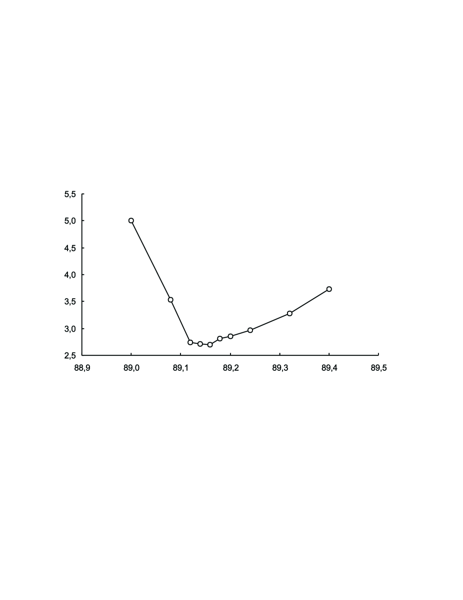
Figure 2: The summary residual (in units $10^{-9}$) depending on the angle of orbital inclination $i$ (in degrees) for optimal values of radii $r_{1}$ and $r_{2}$ .

The numerical experiments shown that global minimum of expression (9) can be found surely enough. In figure 2 presented the summary residual depending on the angle of orbital inclination $i$ for optimal values of radii $r_{1}$ and $r_{2}$ . The values of the geometrical parameters correspond to the global minimum of residual are following: $i=89^{o}.16\pm 0^{o}.02,r_{1}=0.29990\pm 0.00002,r_{2}=0.20005\pm 0.00002$ . Values of errors are formal and equal to steps of the grids used in the carrying out variation of the geometrical parameters.

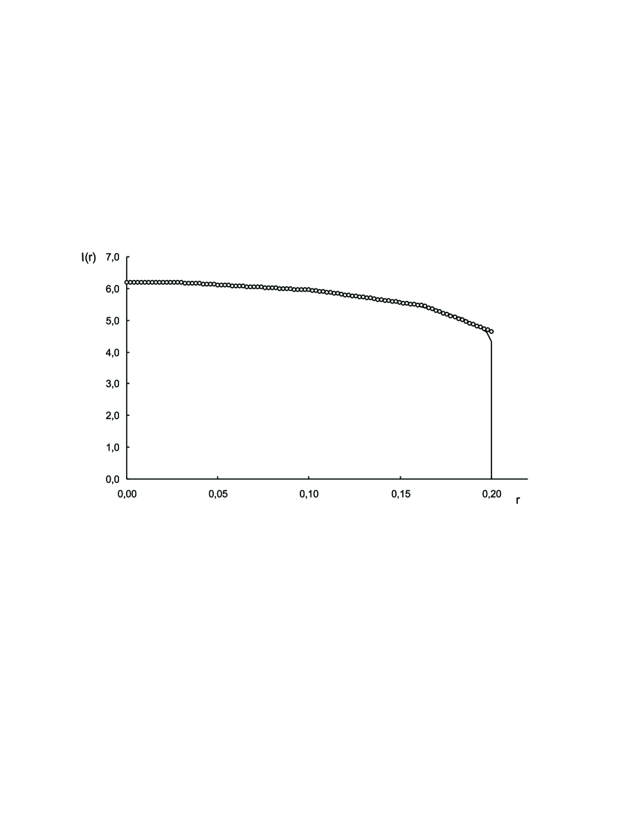
Figure 4: The samples of the restored brightness distribution for the second component (circles) and the precise distribution (solid line).

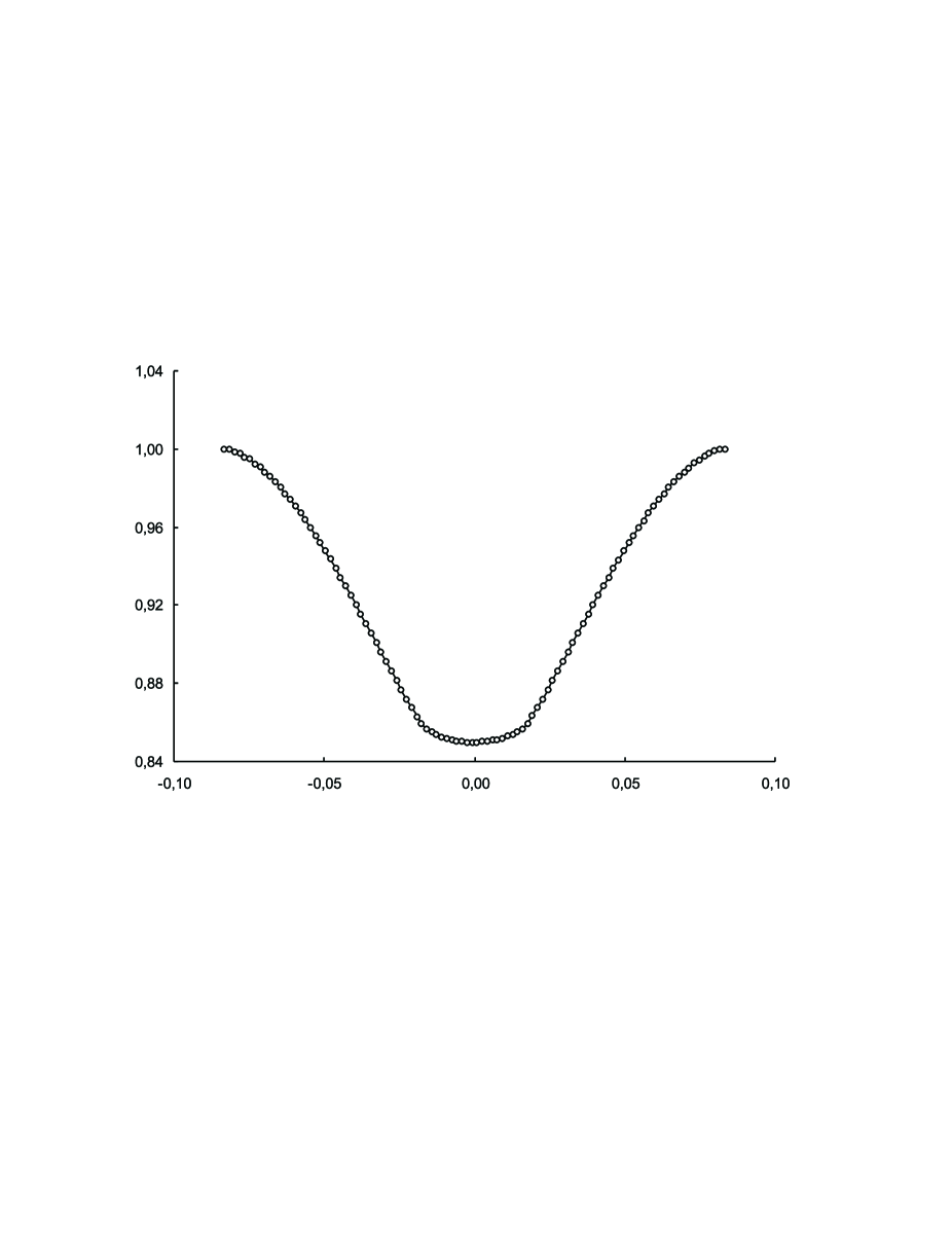
Figure 5: The samples of the perturbed light curve for the secondary minimum (circles) and the light curve correspond to the restored brightness distribution (solid line).

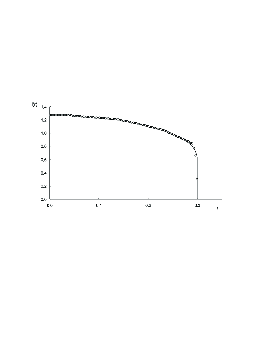
Figure 6: The samples of the restored brightness distribution for the first component (circles) and the precise distribution (solid line).

The samples of the perturbed light curve are presented by circles for the primary minimum in figure 3 and for the secondary minimum - in figure 5. By solid lines in these figures are shown the curves correspond to the restored brightness distributions. The samples of the restored brightness distributions are shown by circles in figure 4 and 6, where also are presented by solid lines the precise distributions. Only each tenth sample is shown in order to avoid of imposition. As can be seen from figures 4 and 6, the accuracy of restoration of the brightness distribution proves to be sufficiently high practically on entire disk of star. Unfortunately, on the edges of disks, at the points of the discontinuity of a function, the solutions are noticeably differed from precise values. This is explained by the absence of the convergence of solution of ill-posed problem at the points of discontinuity of a function.

5. Conclusion

We carried out numerical experiments on the evaluation of the possibilities of obtaining the information about brightness distributions for the components of eclipsing variables from the data of high-precision photometry expected for planned satellites COROT and Kepler. We investigated of both approaches to analysis of light curves: the fitting of the nonlinear model, into the number of parameters of which included the limb darkening coefficients, and the solution of the ill-posed inverse problem of restoration of brightness distributions across the disks of stars with using a priori information about the form of these functions.

It is shown that in both cases the analysis of high-precision data of a space photometry makes it possible to obtain the well concordant results. The standard deviations in the estimations of the model parameters linearly decrease with the decrease of the relative error of the registration of the light curve. If the observational accuracy of the space photometry amounts to $10^{-4}$ (by one order higher than precision of ground-based photometry) then the limb darkening coefficients can be found with the relative error approximately 0.01 . This accuracy will make it possible to easily distinguish the linear law of limb darkening of the nonlinear and to use for its estimation the fitting of more complex models of brightness distributions. The accuracy of restoration of the brightness distribution without rigid model constraints on the form of this function proves to be sufficiently high practically on entire disk of star. Unfortunately, on the edges of disks, at the points of the discontinuity of a function, the solutions are noticeably differed from precise values. The geometric parameters of eclipsing variable, found at the search for the global minimum of residual in case of the restoration of brightness distributions, also prove to be close to the precise values.

References

1. C.Maceroni and I.Ribas, E-print, astro-ph/0511171 (2005).

2. V.P.Tsesevich (Editor), Eclipsing variable stars (Nauka, Moscow, 1971) (in Russian).

3. J.E.Dennis and R.B.Schnabel, Numerical methods for unconstrained optimization and nonlinear equations (Prentice - Hall, Inc., Englewood Cliffs, New Jersey, 1983).

4. A.M.Cherepashchuk, A.V.Goncharskii and A.G.Yagola, Sov. Astron. 11, 990 (1968).

5. A.N.Tikhonov, A.V.Goncharsky, V.V.Stepanov and A.G.Yagola, Regularizing algorithms and a priori information (Nauka, Moscow, 1983) (in Russian).

6. A.M.Cherepashchuk, A.V.Goncharsky and A.G.Yagola, Ill-posed problems in astrophysics (Nauka, Moscow, 1985) (in Russian).

Table 1. The average values of the model parameters and their standard deviations obtained by the model fitting from the primary minimum for different values of relative error of the light curve.

  Para-     Precise                    $\epsilon=10^{-5}$                                   $\epsilon=10^{-4}$                               $\epsilon=10^{-3}$

meter     value  

i               $89^{o}.0$          $88^{o}.9992\pm 0^{o}.0034$                   $89^{o}.001\pm 0^{o}.035$                    $89^{o}.09\pm 0^{o}.41$

$r_{2}$             0.20         $0.1999989\pm 0.0000081$             $0.200002\pm 0.000085$             $0.20006\pm 0.00073$

$L_{2}$            0.70       $0.70000000\pm 0.00000072$          $0.7000002\pm 0.0000074$         $0.700018\pm 0.000078$

$x_{2}$            0.30             $0.29998\pm 0.00024$                     $0.3001\pm 0.0027$                    $0.302\pm 0.023$

$r_{1}$             0.30         $0.3000007\pm 0.0000028$              $0.300000\pm 0.000030$            $0.30000\pm 0.00028$

 

Table 2. The average values of the model parameters and their standard deviations obtained by the model fitting from the secondary minimum for different values of relative error of the light curve.

  Para-     Precise                       $\epsilon=10^{-5}$                               $\epsilon=10^{-4}$                           $\epsilon=10^{-3}$

meter     value  

i               $89^{o}.0$               $88^{o}.994\pm 0^{o}.018$                   $88^{o}.99\pm 0^{o}.15$                  $88^{o}.69\pm 0^{o}.99$

$r_{1}$             0.30              $0.300001\pm 0.000029$            $0.30000\pm 0.00026$             $0.3002\pm 0.0028$

$L_{1}$            0.30              $0.300025\pm 0.000085$            $0.30005\pm 0.00074$             $0.3035\pm 0.0069$

$x_{1}$            0.50                $0.49989\pm 0.00055$                $0.4995\pm 0.0052$                 $0.487\pm 0.056$

$r_{2}$             0.20              $0.199996\pm 0.000017$            $0.20000\pm 0.00016$              $0.1995\pm 0.0015$

 

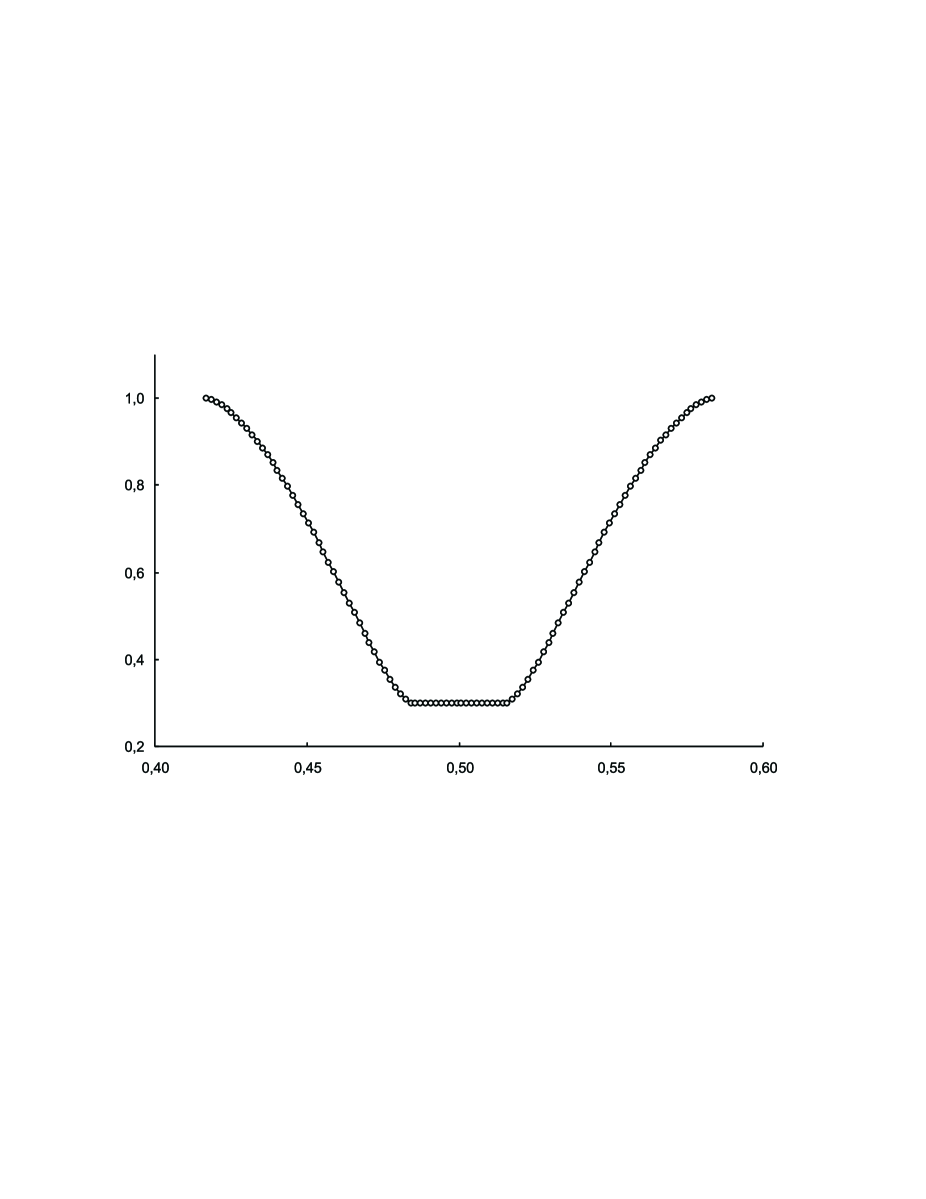
Figure 3: The samples of the perturbed light curve for the primary minimum (circles) and the light curve correspond to the restored brightness distribution (solid line).