Analysis methods for Atmospheric Cerenkov Telescopes

LPNHE
IN2P3 - CNRS - Universités Paris VI/VIII
4 Place Jussieu F-75252 Paris Cedex 05, France

Three different analysis techniques for Atmospheric Imaging System are presented. The classical Hillas parameters based technique is shown to be robust and efficient, but more elaborate techniques can improve the sensitivity of the analysis. A comparison of the different analysis techniques shows that they use different information for gamma-hadron separation, and that it is possible to combine their qualities.

1 Introduction

From the beginning of ground based gamma ray astronomy, data analysis techniques were mostly based on the “Hillas parametrisation” [1] of the shower images, relying on the fact that the gamma-ray images in the camera focal plane are, to a good approximation, elliptical in shape. More elaborate analysis techniques were pioneered by the work of the CAT collaboration on a model analysis technique, where the shower images are compared to a more realistic pre-calculated model of image. Other analysis techniques, such as the 3D Model analysis were developed more recently with the start of the third-generation telescopes. The 3D Model analysis is, for instance, based on the assumption of a 3 dimensional elliptical shape of the photosphere.

These analysis techniques are complementary in many senses. We will show that they are sensitive to different properties of the shower, and can therefore be used to cross-check the analysis results or be combined together to improve the sensitivity. No analysis is currently really winning the race, and there is much space for further improvements.

2 Hillas-parameter based analysis

2.1 Introduction

In a famous paper of 1985[1], M. Hillas proposed to reduce the image properties to a few numbers, reflecting the modelling of the image by a two-dimensional ellipse. These parameters, shown on figure 1, are usually:

• length $L$ and width $w$ of the ellipse

• size (total image amplitude)

• nominal distance $d$ (angular distance between the centre of the camera and the image centre of gravity)

• azimuthal angle of the image main axis $\phi$

• orientation angle $\alpha$

Figure 1: Geometrical definition of the Hillas Parameters.

2.2 Single telescope reconstruction

In single telescope observations, the shower direction was estimated from the Hillas parameters themselves (and in particular from the image length and size), either with lookup tables or with ad-hoc analytical functions. But the choice of a symmetrical parametrisation of the shower led to degenerate solutions, on each side of the image centre of gravity along the main axis.

In order to break this degeneracy, other parameters — based in particular on the third order moments — were added later.

The shower energy is usually estimated with a similar technique, from the image size and nominal distance.

2.3 Stereoscopic reconstruction

The stereoscopic imaging technique, pioneered by HEGRA[3], provides a simple geometric reconstruction of the shower: the source direction is given by the intersection of the shower image main axes in the camera, and the shower impact is obtained in a similar manner. The energy is then estimated from a weighted average of each single telescope energy reconstruction.

2.4 Gamma-hadron separation

The Hillas parameters not only allow to reconstruct the shower parameters, but also can provide some discrimination between $\gamma$ candidates and the much more numerous hadrons. Several technique were developed, exploiting to an increased extent the existing correlation between the different parameters (e.g. Supercuts[7], Scaled Cuts[3] and Extended Supercuts[8]). We will use here the Scaled Cuts technique, in which the actual image width ($w$) and length ($l$) are compared to the expectation value and variance obtained from simulation as a function of the image charge $q$ and reconstructed impact distance $\rho$, expressed by two normalised parameters Scaled Width(SW) and Scaled Length(SL):

$$SW=\frac{w(q,\rho)-\left<w(q,\rho)\right>}{\sigma_{w}(q,\rho)},\quad SL=\frac{l(q,\rho)-\left<l(q,\rho)\right>}{\sigma_{l}(q,\rho)}$$ (1)

These parameters have the noticeable advantage of being easily combined in stereoscopic observations in Mean Scaled Width and Mean Scaled Length:

$$MSW=\frac{\displaystyle\sum_{tels}SW}{\sqrt{ntels}},\quad MSL=\frac{\displaystyle\sum_{tels}SL}{\sqrt{ntels}}$$ (2)

From simulations, one can show that the Mean Scaled Width and Mean Scaled Length are almost uncorrelated for $\gamma$ candidates ($\rho=0.15\pm 0.01$) and can therefore be combined in a single variable Mean Scaled Sum (MSS) : $MSS=(MSW+MSL)/\sqrt{2}$.

3 Model analysis

3.1 Introduction

The Model Analysis, introduced by the CAT collaboration[6] (with a single telescope) and further developed in the H.E.S.S. collaboration[4], is based on the pixel-per-pixel comparison of the shower image with a template generated by a semi-analytical shower development model. The event reconstruction is based on a maximum likelihood method which uses all available pixels in the camera, without the requirement for an image cleaning. The probability density function of observing a signal $S$ in a given pixel, given an expected amplitude $\mu$, a fluctuation of the pedestal $\sigma_{p}$ (due to night sky background and electronics) and a fluctuation of the single photoelectron signal (p.e.) $\sigma_{s}\approx 0.4$ (PMT resolution) is given by the formula:

$$P(S|\mu,\sigma_{p},\sigma_{s})=\sum_{n=0}^{\infty}\frac{e^{-\mu}\mu^{n}}{n!\sqrt{2\pi(\sigma_{p}^{2}+n\sigma_{s}^{2})}}\exp\left(-\frac{(S-n)^{2}}{2(\sigma_{p}^{2}+n\sigma_{s}^{2})}\right)$$ (3)

The log-likelihood function ${\cal L}=2\sum_{\mathrm{pixel}}\log\left[P_{i}(S_{i}|\mu,\sigma_{p},\sigma_{s})\right]$ is then maximised to obtain the primary energy, direction and impact. In contrast to the Hillas Analysis technique, the shower reconstruction works in an identical way for a single telescope or for a stereoscopic array.

In stereoscopic observations, the Model analysis uses by its nature the correlations between the different images to find the best source direction and position, but in contrast to the Hillas analysis, it doesn’t take into account the shower fluctuations.

3.2 Gamma-hadron separation

In the Model analysis, the separation between the $\gamma$ candidates and the hadrons is done by a goodness-of-fit ($G$) variable. The average value of the log-likelihood can be calculated analytically:

$$\left<\ln{\cal L}\right> = \sum_{pixel\,i}\int_{S_{i}}P(S_{i}|\mu_{i},\sigma_{p_{i}},\sigma_{s_{i}})\times\ln P(S_{i}|\mu_{i},\sigma_{p_{i}},\sigma_{s_{i}})\,dS_{i}$$ (4)

$$= \sum_{pixel\,i}\left[1+\ln(2\pi)+\ln\left(\sigma_{p_{i}}^{2}+\mu_{i}\times(1+\sigma_{s_{i}}^{2})\right)\right]$$

The variance of $\ln{\cal L}$ being close to 2, we define the goodness-of-fit $G$ as a normal variable ($N_{\mathrm{dof}}$ is the number of degrees of freedom):

$$G=\frac{\left<\ln{\cal L}\right>-\ln{\cal L}}{\sqrt{2\times N_{\mathrm{dof}}}}$$ (5)

4 3D Model analysis

4.1 Introduction

The third and most recent analysis presented here, the 3D Model Analysis[5], is a kind of 3 dimensional generalisation of the Hillas parameters: the shower is modelled as a Gaussian photosphere in the atmosphere (with anisotropic light angular distribution), which is then used to predict — with a line of sight path integral — the collected light in each pixel. A comparison of the actual image to the predicted one (with a log-likelihood function) allows eight shower parameters to be reconstructed: mean altitude, impact and direction, 3D width and length and luminosity.

Reconstructed parameters:

• mean altitude

• impact

• direction

• 3D width and length

• luminosity

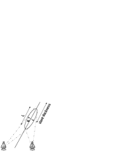
Figure 2: Geometrical definition of the 3D Model Parameters.

4.2 Gamma-Hadron separation

The 3D-Model analysis relies on the strong assumption of a rotational symmetry, which is used to reject about 70% of the hadrons during the fit procedure. For the remaining events, the most discriminating parameter between the $\gamma$ candidates and the hadrons is found to be the shower width, as the hadronic showers are typically much wider than the electromagnetic ones. The shower width, expressed in units of radiation length, is found by simulation to be proportional to the slant thickness. This is is used to define a zenith angle independent Reduced width parameter:

$$\omega=\frac{w\times\rho{z_{\mathrm{max}}}}{\mathrm{thickness}}$$ (6)

For simplicity, we will use here a Rescaled width ($Wr_{3D}$) parameter constructed from the Reduced width with a fixed offset and a fixed ratio, to be a Gaussian distributed variable with mean 0 and RMS 1.

5 Comparison

In this section we compare the properties of the three analyses presented above. For that purpose, we will use two data sets:

• a real data set of 10 live hours obtained by H.E.S.S. on the Crab Nebula in 2004 with 3 telescopes.

• a simulation data set at zenith.

5.1 Selection variables and efficiency

The distributions of the three discriminating parameters (Mean Scaled Sum, Goodness and Rescaled Width) are shown in figure 3 for simulated $\gamma$’s, real OFF data and real ON-OFF data. For the three analyses, the real ON-OFF distributions are well reproduced by the simulation and are compatible with normal variables. The OFF distributions have a different shape, indicating that a cut $V\leq V_{\mathrm{max}}$ on these variables can be used.

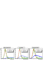
Figure 3: Distribution of discriminating parameters obtained for each analysis for simulated $\gamma$’s, real OFF data and real $\gamma$ obtained from ON-OFF data. Left: Mean Scaled Sum, Middle: Model Goodness of Fit, Right: 3D Model Rescaled Width.

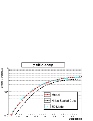
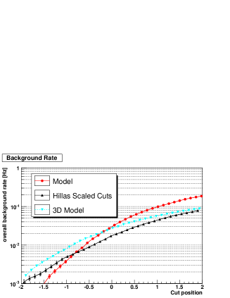
Figure 4: Left: efficiency of the three analyses to simulated $\gamma$ with respect to the cut position. Right: remaining background rate (from real data) for the same cuts.

Figure 4 shows the efficiency of the three analyses for a point source at zenith, including the reconstruction efficiency and the efficiency of a $\theta^{2}\leq 0.02$ cut, as a function of the position of $V_{\mathrm{max}}$. The three curves on the left panel are very similar in shape, reflecting the fact that the selection variables all have a normalised Gaussian distribution. The Model and 3D Model analyses have a $\sim 20\%$ higher efficiency for $\gamma$-rays compared to the Hillas parameters based method, partially thanks to a higher reconstruction efficiency and partially due to a slightly better angular resolution. They also keep more background events, which in turns leads to very similar sensitivities (table 2).

5.2 Discriminating parameters correlations

Since the three analysis presented here have similar sensitivities and $\gamma$ efficiencies, one would expect to see a strong correlation between the discriminating variables. Figure 5 shows the distribution of Model goodness-of-fit versus Hillas Mean Scaled Goodness for simulated $\gamma$’s (left) and real OFF data (right).

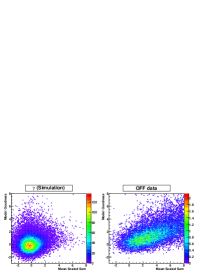
Figure 5: Correlation of selection variables for two different analyses on the same events.

The surprise is that there is almost no correlation between these variables for simulated $\gamma$’s (correlation factor $\rho\approx 0.13$) whereas there is some for the OFF data ($\rho\approx 0.53$). The same effect is seen when comparing the Hillas analysis to the 3D Model, or the 3D Model with the Model. The obtained correlation factors are summarised in the table 1.

Coefficient	$\gamma$ (Simulation)	OFF data
Model / Hillas	$0.126\pm 0.004$	$0.53\pm 0.02$
3D Model / Hillas	$0.03\pm 0.004$	$0.51\pm 0.02$
3D Model / Model	$0.120\pm 0.004$	$0.35\pm 0.02$

Table 1: Correlation between the discriminating variables of the three describes analyses, for simulated $\gamma$’s and real OFF data.

The reason of this lack of correlation is not perfectly clear yet, but it must certainly be due to the fact that the analyses are sensitive to different shower properties:

• The Hillas - Scaled cuts analysis takes into account the shower development fluctuations (in the construction of the scaled cuts tables), but doesn’t take into account the details of the light distribution inside the shower image (and in particular its asymmetry), nor the correlations between the images

• The Model analysis takes into account the details of the light distribution and the correlations between the images but not the shower fluctuations

• The 3D Model analysis takes into account the correlations between the images, and some aspects of the details of light distribution as well as the shower fluctuations (through their effect on the shower length and width).

This also shows that none of these analyses completely exploits the available information, and that significant improvements can be achieved. In particular, it’s is possible to combine the selection variables by simpling adding them. We define two new discriminating variables $V2$ and $V3$:

$$V2=\frac{MSS+G}{\sqrt{2}},\quad\quad V3=\frac{MSS+G+Wr_{3D}}{\sqrt{3}}$$ (7)

The results obtained on the Crab data sample with the three analysis, using the same cut position ($V2\leq 0.8$ or $V3\leq 0.8$ ), a 60 photoelectrons cut and a 2 degrees Nominal distance cut (to remove the events close to the edge of the camera) are shown together with the results of the combined cuts $V2$ and $V3$ in table 2. It should be noted that the average zenith angle of the Crab dataset is roughly $40^{\circ}$ and that this dataset was taken with 3 telescope, so the actual $\gamma$ efficiency and hadron rejection cannot be directly compared to the values obtained on simulation in figure 4.

Analysis	ON	OFF	$\#\gamma$	$\sigma$	S/B	$\sigma_{10}$
Model ($G\leq 0.8$)	2725	481	2244	41.6	4.5	6.5
Hillas ($MSS\leq 0.8$)	1979	254	1725	38.9	7.0	6.6
3D Model ($Wr_{3D}\leq 0.8$)	1908	309	1599	35.8	5.2	5.7
Model/Hillas ($V2\leq 0.8$)	2587	225	2362	48.2	10.5	9.1
3 analysis ($V3\leq 0.8$)	2197	165	2032	45.6	13.1	9.5

Table 2: Results of the three analyses and the combined analysis on a Crab data set. For each analysis, we quote the number of ON and OFF events, the number of $\gamma$, the significance, the signal over background ratio and the significance obtained for a 10 times fainter source.

Even for a strong source, the significance is noticeably increased when combining the analyses together. For faint sources, the gain in significance is almost $40\%$, due to a two times better background rejection for roughly the same $\gamma$ acceptance.

5.3 Resolution

Comparing the angular or energy resolution between different analysis is always a tricky business, since the values obtained depend in particular on the selection criteria which are specific to each analysis. The clean way to do it is to use a common sample of events. We use here the events selected with $V3\leq 0.8$, which does not favour any analysis with respect to the others.

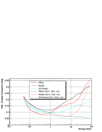
Figure 6: Angular resolution of the three analysis methods as function of energy, with and without nominal distance cut.

The results of the angular resolution comparison is shown in figure 6, with and without nominal distance cut. For all analyses, applying a nominal distance cut rejects the high energy events falling far away from the telescope (which have almost parallel images in the telescopes) thus improving the angular resolution at the expense of a much smaller effective area (by a factor of typically 5 at 10 TeV). The Model analysis performs significantly better than other analyses at low energy whereas the 3D Model takes over at higher energies.

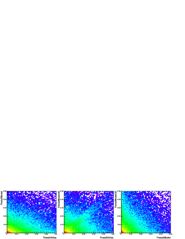
Figure 7: Correlation of the reconstructed squared angular distance to true shower axis ($deg^{2}$) between respectively the Hillas and Model analyses (left), the Hillas and 3D Model analyses (middle) and the Model and 3D Model analyses (right).

More interestingly, figure 7 shows the correlation of the reconstructed squared angular distance to shower true direction ($\theta^{2}$) between the three analyses. The values of $\theta^{2}$ are not very much correlated (correlation factors between $0.3$ and $0.5$) between the analyses. This has been identified to be due to different reconstructions patterns on the ground: The Hillas analysis best reconstructs the events that are well within the array, whereas the Model analysis performs better with events that are not too close to one telescope. The 3D Model does its best with high telescope-multiplicity events, which concentrates at the center of the array.

5.4 Off-axis observations

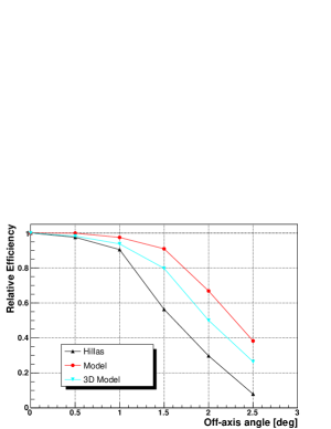
Figure 8: Relative efficiency to $\gamma$-rays of the 3 analyses as a function of distance to camera centre.

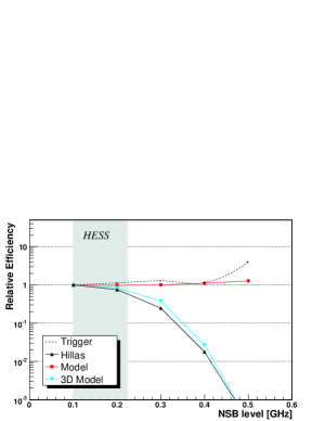
Figure 9: Relative efficiency to $\gamma$-rays of the 3 analyses as a function of night sky background level.

Figure 9 shows the relative evolution of the efficiency for $\gamma$-rays as function of the OFF-axis angle (distance of the shower axis to the centre of the camera) for the three analyses. As expected, the efficiency of the Hillas analysis starts to fall off before the others: the efficiency of the Mean Scaled Width/Length parameters degrades quickly due to truncated showers. Neither the Model nor the 3D Model analysis relies on the actual — truncated — images but rather extrapolate the available information and have therefore a flatter efficiency.

5.5 Sensitivity to Night Sky Background

The variation of the efficiency to $\gamma$-rays with respect to the Night Sky Background level (NSB) is shown for the three analyses considered in figure 9. The efficiency of the Hillas and the 3D Model analyses both start to drop quickly above 200 MHz, whereas the efficiency of the Model analysis is much flatter, due to its complete treatment of the NSB level in the goodness-of-fit parameter.

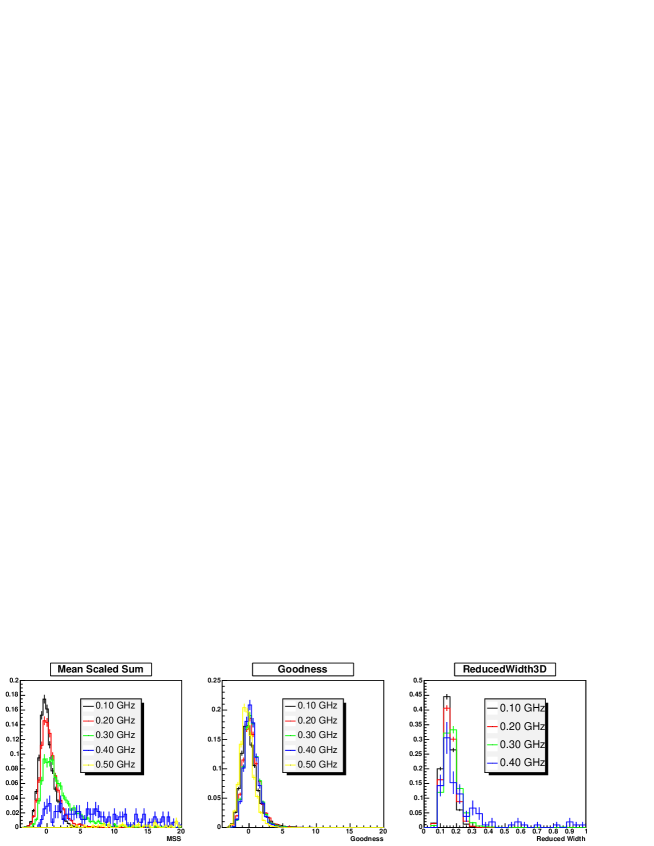
Figure 10: Evolution of the three discriminating parameter distributions as a function of the Night Sky Background level.

Figure 10 shows the evolution of the three discriminating parameter (Mean Scaled Sum, Goodness-of-fit and Reduced 3D Width) distributions as a function of the Night Sky Background level. As for the OFF-axis efficiency, the degradation of the Mean Scaled Width/Length parameters is responsible for the efficiency drop of the Hillas analysis, whereas the 3D Model seems to suffer mainly from convergence problems which might be solved in the future. As expected, the Model Goodness-of-fit distribution remains stable as the NSB level changes. It should be noted however that in the operational region of the current telescopes (100 - 200 MHz for HESS), the efficiency of all three analyses remains almost flat.

6 Conclusion

We have presented three completely different analysis methods for Atmospheric Cerenkov Telescopes. These three methods show similar efficiencies, although they are sensitive to different properties of the shower. The intrinsic capabilities of each analysis (and it particular the hadronic rejection capabilities) can be combined together to improve the sensitivity of the analysis. Since these three analyses perform differently in different energy and impact parameter domain, more detailed studies should also allow to use the select on an event-per-event basis the optimal response and therefore improve the quality (angular resolution,…) of the analysis.

References

- [1] A. Hillas, “Cerenkov light images of EAS produced by primary gamma”, Proc. 19nd I.C.R.C. (La Jolla), Vol 3, 445 (1985)
- [2] W. Hofmann et al, “Comparison of techniques to reconstruct VHE gamma-ray showers from multiple stereoscopic Cherenkov images”, Astropart. Phys. 12, 135 (1999)
- [3] A. Daum et al, “First results on the performance of the HEGRA IACT array”, Astropart. Phys. 8, 1 (1997)
- [4] M. de Naurois et al, “Application of an Analysis Method Based on a Semi-Analytical Shower Model to the First H.E.S.S. Telescope”, Proc. 28nd I.C.R.C. (Tsukuba), Vol 5, 2907 (2003)
- [5] M. Lemoine-Goumard et al, “3D-reconstruction of gamma-ray showers with a stereoscopic system”, these proceedings pp. LABEL:Lemoine-GoumardStart-LABEL:Lemoine-GoumardEnd
- [6] F. Piron et al, “Temporal and spectral gamma-ray properties of Mkn 421 above 250 GeV from CAT observations between 1996 and 2000”, A&A 374, 895 (2001)
- [7] P. T. Reynolds et al, “Survey of candidate gamma-ray sources at TeV energies using a high-resolution Cerenkov imaging system - 1988-1991”, ApJ 404, 206 (1993)
- [8] G. Mohanty et al, “Measurement of TeV gamma-ray spectra with the Cherenkov imaging technique”, Astropart. Phys. 9, 15 (1998)