The halo mass function from the dark ages through the present day

Abstract

We use an array of high-resolution N-body simulations to determine the mass function of dark matter haloes at redshifts 10-30. We develop a new method for compensating for the effects of finite simulation volume that allows us to find an approximation to the true “global” mass function. By simulating a wide range of volumes at different mass resolution, we calculate the abundance of haloes of mass $10^{5-12}$ $h^{-1}{\rm{M}}_{\odot}$. This enables us to predict accurately the abundance of the haloes that host the sources that reionize the universe. In particular, we focus on the small mass haloes ($\lower 2.15277pt\hbox{\mbox{$\;\buildrel>\over{\sim}\;$}}10^{5.5-6}h^{-1}{\rm{M}}_{\odot}$) likely to harbour population III stars where gas cools by molecular hydrogen emission, early galaxies in which baryons cool by atomic hydrogen emission at a virial temperature of $\sim 10^{4}$K ($\sim 10^{7.5-8}h^{-1}{\rm{M}}_{\odot}$), and massive galaxies that may be observable at redshift $\sim$10. When we combine our data with simulations that include high mass haloes at low redshift, we find that the best fit to the halo mass function depends not only on linear overdensity, as is commonly assumed in analytic models, but also upon the slope of the linear power spectrum at the scale of the halo mass. The Press-Schechter model gives a poor fit to the halo mass function in the simulations at all epochs; the Sheth-Tormen model gives a better match, but still overpredicts the abundance of rare objects at all times by up to 50%. Finally, we consider the consequences of the recently released WMAP 3-year cosmological parameters. These lead to much less structure at high redshift, reducing the number of $z=10$ “mini-haloes” by more than a factor of two and the number of $z=30$ galaxy hosts by more than four orders of magnitude. Code to generate our best-fit halo mass function may be downloaded from http://icc.dur.ac.uk/Research/PublicDownloads/genmf_readme.html

1 introduction

The numbers of haloes in the high redshift universe are critical for determining the numbers of stars and galaxies at high redshift, for understanding reionization, and for guiding observational campaigns designed to search for the first stars and galaxies. The reionization of the universe is thought to be caused by some combination of metal-free stars, early galaxies and accreting black holes (see e.g. Bromm & Larson 2004; Ciardi & Ferrara 2005; Reed et al. 2005 and references therein), all of which are expected to lie in dark matter haloes, the numbers of which are, to date, highly uncertain at these early times. This paper presents an array of cosmological simulations of a wide range of volumes with which we determine the numbers of haloes over the entire mass range that is expected to host luminous sources in the high redshift universe.

The first galaxies are expected to form within haloes of sufficiently high virial temperature to allow efficient cooling by atomic hydrogen via collisionally induced emission processes, which become strong at temperatures of $\sim$10⁴K, providing the possibility of efficient star formation. Haloes of mass $\sim 10^{8}\times[10/(1+z)^{3/2}]$ $h^{-1}{\rm{M}}_{\odot}$ have the required virial temperature to host galaxies. Haloes with virial temperature less than the threshold for atomic hydrogen line cooling, but larger than $\sim$2,000K, often referred to as “mini-haloes”, have the potential to host metal-free (population III) stars that form from gas cooled through the production of H₂ and the resulting collisionally-excited line emission. The first stars in the universe are expected to form within such mini-haloes, which have masses as small as $\sim 10^{5-6}h^{-1}{\rm{M}}_{\odot}$ at redshifts of $\sim$10-50. The inability of collapsing H₂-cooled gas to fragment to small masses, demonstrated in pioneering simulations by Abel, Bryan, & Norman (2000, 2002) and by Bromm, Coppi, & Larson 1999, 2002), suggests that these first stars will be very massive ($\lower 2.15277pt\hbox{\mbox{$\;\buildrel>\over{\sim}\;$}}100{\rm{M}}_{\odot}$), luminous, and short lived, and will thus have dramatic effects on their surroundings. These population III stars begin the process of enriching the universe with heavy elements, and are expected to have an important impact (directly or indirectly) on reionization.

Early estimates of the numbers of haloes in the pre-reionized and the reionizing universe have relied upon analytic arguments such as the Press & Schechter (1974) formalism or the later Sheth & Tormen (1999; S-T) function (further detailed in Sheth, Mo, & Tormen 2001; Sheth & Tormen 2002). For haloes at very high redshifts, which form from rare fluctuations in the density field, these analytic methods are in poor agreement with each other. At lower redshifts, halo numbers have been extensively studied using N-body simulations of large volumes. Simulations by Jenkins et al. (2001) show that the mass function of dark matter haloes in the mass range from galaxies to clusters is reasonably well described by the Sheth & Tormen (1999) analytic function out to redshift 5, although with some suppression at high masses. Jenkins et al. proposed an analytic fitting formula for the “universal” mass function in their simulations. Warren et al. (2006) used a suite of simulations to measure the redshift zero mass function to high precision. Reed et al. (2003) used higher resolution simulations to show that the broad agreement with the S-T function persists down to dwarf scales and to $z=10$, a result that was confirmed by the larger “Millennium” simulation of Springel et al. (2005). However, at $z\simeq 15$, Reed et al. (2003) also found fewer haloes than predicted by the S-T function. Qualitatively consistent results have been found by Iliev et al. (2006), Zahn et al. (2006). These studies indicate that current analytic predictions of halo numbers are inaccurate at high redshift and demonstrate the need for N-body studies to determine the mass function at earlier times.

Early attempts to simulate the formation of dark matter haloes in the young universe suffered from effects resulting from the finite box sizes of the simulations, as noted by (e.g. White & Springel 2000; Barkana & Loeb 2004). Recently Schneider et al. (2006) have modelled haloes large enough to host galaxies using PINOCCHIO (Monaco et al. 2002; Monaco, Theuns, & Taffoni 2002), a code that predicts mass merger histories given a linear density fluctuation field. More directly, Heitmann et al. (2006) used N-body simulations to show that haloes large enough to cool via atomic hydrogen transitions, and thus with the potential to host galaxies at redshifts 10 - 20, are well fit by the Warren et al. mass function, with the largest haloes suppressed relative to the S-T function by an amount consistent with that seen in Reed et al. (2003).

Formation of the first haloes large enough to host galaxies occurs as early as $z\sim 35$ (e.g. Gao et al. 2005; Reed et al. 2005), much earlier than the epochs at which the mass function has been calculated directly. The abundance of smaller haloes, capable of hosting population III stars, but too cool for atomic cooling, remains poorly constrained by numerical simulations; see however early work by Jang-Condell & Hernquist (2001). The major difficulty is the computational challenge of performing simulations with very high mass resolution within a volume that is large enough to sample fully the cosmological mass perturbation spectrum. At high redshifts, the effects of finite box size become particularly important because the haloes to be sampled represent rare fluctuations in the linear fluctuation spectrum. Since the mass function is steep, the numbers of such rare haloes are particularly sensitive to large scale, low amplitude density fluctuations. Finite box size effects worsen as one attempts to simulate the smaller volumes needed to resolve lower mass haloes because fluctuations on the scale of the box become comparable to those on the scale of the halo. In $\Lambda$CDM cosmologies with spectral slope parameter $n_{s}=1$, the effective, local spectral index of the perturbation spectrum, $n_{\rm eff}$, approaches $-3$ on the smallest scales, implying that fluctuations on a broad range of scales have similar amplitude (see further discussion in § 2) . As a result, proper modelling of the power on scales much larger than the scale of the halo is important. Simulations of small haloes must therefore have a large dynamic range in order to model accurately all of the fluctuations that determine the formation and evolution of a halo.

Several authors have estimated the effect of the finite simulation box size on the halo mass function using techniques based on assuming a simple cutoff in the power spectrum of density fluctuations on scales larger than the box length (Barkana & Loeb 2004; Bagla & Ray 2005; Power & Knebe 2006; Bagla & Prasad 2006). While these techniques are able to account for the missing large-scale power, they do not account for cosmic variance, i.e. the run-to-run variations introduced by the finite sampling of density modes, particularly at scales near the box size (e.g. Sirko 2005). Since the density field is derived from a set a discrete Fourier modes with maximum wavelength equal to the box size, the power at the largest wavelengths is determined by only a small number of realised modes. As a result, each random realisation of a simulation volume produces different large-scale structures.

We introduce a technique, described in Section 2, which deals with the finite volume effects through a mass-conserving transformation of the halo mass function estimated from each individual simulation output. In order to verify the ability of this technique to account for finite volume affects, we perform simulations of a wide, but closely spaced range of volumes, which results in large overlaps in redshift and in the range of resolved halo masses in different simulations. The agreement of the inferred mass functions in the regimes where halo masses overlap allows us to verify the finite volume correction, and also allows us to rule out resolution dependencies of our results. Multiple realisations of a single volume at identical resolution then test how well the correction to the inferred mass function is able to minimise the effects of cosmic variance.

Our simulations are designed to extend the mass function to small masses and high redshifts, covering a mass range of $10^{5}$ to 10¹² $h^{-1}{\rm{M}}_{\odot}$, at redshifts 10 to 30, and we supplement them with low redshift data taken from other studies. This extends the mass function down to masses small enough to include the “mini-haloes” capable only of hosting stars formed via H₂-cooling, and determines more precisely the mass function of larger haloes which can host galaxies. In § 2, we define the halo mass function and outline our method for dealing with finite volume effects. In § 3, we discuss our suite of simulations of varying box sizes and resolutions. In § 4, we demonstrate the effectiveness of our techniques for correcting for finite volume and cosmic variance. We then present our mass function and compare it to previous works. In § 5, we consider the dependence of the mass function on cosmological parameters in the light of the recent WMAP third year results (Spergel et al. 2006). In § 6, we discuss some implications of our mass function for astrophysical models that rely on the mass function of high redshift haloes. Finally, our conclusions are summarised in § 7.

Except when otherwise indicated, we assume throughout a flat $\Lambda$CDM model with the following cosmological parameters, which are consistent with the combined first year WMAP/2dFGRS results (Spergel et al. 2003): matter density, $\Omega_{m}=0.25$; dark energy density, $\Omega_{\Lambda}=0.75$; baryon density, $\Omega_{\rm baryon}=0.045$; fluctuation amplitude, $\sigma_{\rm 8}=0.9$; Hubble constant $h=0.73$ (in units of 100 km s^-1 Mpc^-1); and no tilt (i.e. a primordial spectral index of 1). Note that our results should, in principle, be scalable to other values of cosmological parameters.

2 The halo mass function

In this section we define the notation that we use to describe the halo mass function and introduce our method for estimating the halo mass function from our N-body simulations. The simulations themselves are described in § 3.

2.1 Definitions

The differential halo mass function, or halo mass function for short, ${\rm d}n/{\rm d}M$, is defined as the number of haloes of mass $M$ per unit volume per unit interval in $M$. In this section, we introduce, for reasons that will become apparent later, an alternate pair of variables, $f(\sigma)$ and $\ln\sigma^{-1}$, to describe the halo mass function. The quantity $\sigma$ is the RMS linear overdensity of the density field smoothed with a top-hat filter with a radius that encloses a mass $M$ at the mean cosmic matter density. For an infinite volume we have:

$$\sigma^{2}(M)={b^{2}(z)\over 2\pi^{2}}\int_{0}^{\infty}k^{2}P(k)W^{2}(k;M){\rm d}k,$$ (1)

where $P(k)$ is the linear power spectrum of the density fluctuations at $z=0$, $W(k;M)$ is the Fourier transform of the real-space top-hat filter, and ${\it b(z)}$ is the growth factor of linear perturbations normalised to unity at $z=0$ (Peebles 1993). The quantity $\ln\sigma^{-1}$ can be thought of as a mass variable in the sense that higher values of $\ln\sigma^{-1}$ correspond to higher masses for a given redshift and matter power spectrum.

The quantity, $f(\sigma)$, to which we will refer as the mass function, is defined as the fraction of mass in collapsed haloes per unit interval in $\ln\sigma^{-1}$. If all matter is in haloes of some mass then:

$$\int_{-\infty}^{\infty}f{\rm~{}d}\ln\sigma^{-1}=1.$$ (2)

The differential halo mass function is related to $f(\sigma)$ by:

$${{\rm d}n\over{\rm d}M}={\rho_{0}\over M}{{\rm d}\ln\sigma^{-1}\over{\rm d}M}f(\sigma),$$ (3)

where $\rho_{0}$ is the mean mass density of the universe.

The function $f(\sigma)$ will depend on how haloes are defined. For this paper, in common with most recent work on halo mass functions, we use the friends-of-friends (FOF) algorithm (Davis et al. 1985) with a linking length of 0.2 times the mean inter-particle separation. In the appendix we include mass functions using the SO algorithm (Lacey & Cole 1994).

The reasons for choosing to describe the halo mass function in terms of the rather abstract variables $f$ and $\ln\sigma^{-1}$ are twofold. Firstly, the most commonly used analytical halo mass functions can be expressed compactly in terms of these variables. For example, the Press & Schechter (1974; P-S) mass function can be expressed as:

$$f_{\rm P-S}(\sigma)=\sqrt{2\over\pi}{\delta_{c}\over\sigma}\exp\bigg{[}-{\delta_{c}^{2}\over 2\sigma^{2}}\bigg{]},$$ (4)

where the parameter $\delta_{c}=1.686$ can be interpreted physically as the linearly extrapolated overdensity of a top-hat spherical density perturbation at the moment of maximum compression for an Einstein de-Sitter universe ($\Omega_{m}=1$). The evolution of $\delta_{c}$, predicted by the spherical collapse model (e.g. Eke, Cole & Frenk 1996) as $\Omega_{m,z}$ transitions from $\simeq 1$ at high redshift to its present value, is sufficiently weak that we have ignored it in our treatment. Similarly, the Sheth-Tormen (S-T) mass function takes the form:

$$f_{\rm S-T}(\sigma)=A\sqrt{{2a\over\pi}}\bigg{[}1+\big{(}{\sigma^{2}\over a\delta_{c}^{2}}\big{)}^{p}\bigg{]}{\delta_{c}\over\sigma}\exp\bigg{[}-{a\delta_{c}^{2}\over 2\sigma^{2}}\bigg{]}.$$ (5)

The choice of values $A=0.3222$, $a=0.707$ and $p=0.3$ provides a significantly better fit to mass functions determined from numerical simulations over a wide range of masses and redshifts than the P-S formula.

Secondly, it has been found empirically, consistently with the analytic mass function formulae above, that the FOF mass function determined from cosmological simulations for a wide range of redshifts, and for a wide range of cosmological models can be fitted accurately by a unique function $f(\sigma)$ (e.g. S-T 1999, Jenkins et al. 2001, Reed et al. 2003, Linder & Jenkins 2003, Lokas, Bode & Hoffmann 2004, Warren et al. 2006). A number of formulae for $f(\sigma)$ have been proposed based on fits to simulation data and these are generally consistent at the $\sim$10-30% with the largest differences occuring at the high mass end, where the rarity and steepness of the halo mass function make its estimation rather challenging. The main aim of this paper is to determine the halo mass function at high redshift and to provide a fitting formula which applies to both our high and low redshift simulation data.

It is appropriate here to question whether the halo mass function can really be expressed as a universal function of the form $f(\sigma)$ (see further discussion in S-T 1999). Structure formation in Einstein-deSitter cosmological N-body simulations in which the initial power spectrum is a (truncated) power-law ($P(k)\propto k^{n}$) has been found to show self-similar evolution (e.g. Efstathiou et al. 1998, Lacey & Cole 1994). For a given value of $n$, self-similar evolution implies a universal form for $f(\sigma)$. However the function $f$ could, in principle, be different for different values of the power-law index, $n$. There is suggestive evidence that this may indeed be the case in Fig. 1 of Lacey & Cole (1994).

Thus, while empirically the CDM halo mass function appears to be well described by a function $f(\sigma)$, it may be that it is possible to improve the accuracy of a fitting formula by adding an additional parameter. For the CDM power spectrum where the slope curves gently a natural parameter to take would be the local slope of the power spectrum. At the small spatial scales relevant to the halo mass function at high redshift, the spectral slope approaches a critical value $n=-3$ which marks the boundary between bottom-up hierarchical structure formation and top-down structure formation. One might expect that the need for an extra parameter would become apparent as this boundary is approached. In § 4.2, we find that we can improve the goodness of fit to our mass function by using this as an extra parameter, and it is the high redshift simulation data which require this.

2.2 Finite simulations and the global mass function

Due to limited computing resources any cosmological N-body simulation can only model a finite volume of space. Periodic boundary conditions are usually implemented in order to avoid edge effects, with the most common geometry being a periodic cube. In this case, the overdensity of matter, $\delta({\bf r})$, is given by a sum over Fourier modes:

$$\delta=\sum_{\bf k}\delta_{\bf k}\exp(i{\bf k}.{\bf r}),$$ (6)

where the $\delta_{\bf k}$ are complex amplitudes which obey a reality condition $\delta_{\bf k}^{*}=\delta_{\bf-k}$. Because the simulation volume must have mean density, $\delta_{\bf k=0}=0$. The Fourier modes have wavenumbers ${\bf k}=2\pi/L_{\rm box}(l,m,n)$, where $l,m,n$ are integers and $L_{\rm box}$ is the side-length of the simulation volume.

The initial conditions for a simulation of a CDM universe with adiabatic density perturbations require that the initial density field should be a Gaussian random field. In this case, the phases of the wave amplitudes, $\delta_{\bf k}$, are random, and the amplitude of each mode is drawn from a Rayleigh distribution (Efstathiou et al. 1985) where:

$$<|\delta_{\bf k}|^{2}>=P(k)/L_{\rm box}^{3}$$ (7)

and the brackets $<>$ denote an ensemble average over realisations.

For a periodic cosmological simulation, the smoothed rms linear overdensity, $\sigma$, is given by the discrete analog of Eqn. 1:

$$\sigma^{2}(M)={b^{2}}(z)\sum_{\bf k}|\delta_{\bf k}|^{2}W^{2}(k;M),$$ (8)

where $|\delta_{\bf k}|$ refers to the linear amplitude of the Fourier modes at $z=0$, and $b$ and $W$ are the same as in Eqn. 1.

A number of authors (Power & Knebe 2006; Sirko 2005; Bagla & Prasad 2006) have highlighted the problem that the halo mass function in a finite periodic box will differ between realisations and that the ensemble average mass function will not be the same as in the limit of an infinitely large simulation volume. The effects of having a discrete power spectrum with only a small number of modes with wavelengths comparable to the size of the cube and no power with wavelengths larger than the cube are particularly important for small cosmological volumes where the contribution to the variance of the density field from each successive decade of wavenumber is a very weakly increasing function. Given the computing resources available to us and the requirement that we should resolve haloes with a hundred or more particles at high redshift, it is inevitable that the volumes we wish to simulate will be affected significantly by finite box effects.

Our approach to minimise finite box effects and to estimate the high redshift halo mass function is to make the ansatz that the universal form of the halo mass function correctly describes the halo mass function even in volumes where finite volume effects are significant. For small volumes it is important to use the correct relation between $M$ and $\sigma$ given by Eqn. 8 for each individual simulation in order to estimate the halo mass function in $f(\sigma)-\ln\sigma^{-1}$ space. Having estimated $f(\sigma)$ we can now predict the halo mass function, Eqn. 3 for the astrophysically interesting case of an infinite volume, using the relation between $\sigma$ and $M$ given by Eqn. 1. We call this mass function the global mass function.

It not obvious a priori just how successful this approach will be in recovering the global mass function. However, it is worth noting that this approach contains inherently the essential elements present in conditional mass function methodology wherein the number of haloes within a local patch is estimated (Mo & White 1996, Bower 1991, Bond et al. 1991, Lacey & Cole 1993). If we take our simulation volume to be a patch of universe with mass $M_{\rm patch}$ and mean density, then the variance that we measure within the simulation volume is close to $\sigma^{2}_{\rm global}(M)-\sigma^{2}_{\rm global}(M_{\rm patch})$, where $\sigma^{2}_{\rm global}(M)$ is given by Eqn. 1. The mass function in such a finite patch is reliably predicted by substituting $\sigma^{2}_{\rm global}(M)-\sigma^{2}_{\rm global}(M_{\rm patch})$ for $\rm\sigma^{2}_{\rm global}(M)$ into the functional form of the mass function (Sheth & Tormen 2002). Our methodology is an improvement on such an approach because we also include the effects of run to run “cosmic” variance. As will be discussed in § 4, we find that our method does work very well in practice. To demonstrate this one needs a large number of simulations with multiple random realisations at a fixed box size and a variety of differing box sizes. We describe our suite of simulations in the next Section.

In practice, we determine $\sigma(M)$ for a particular simulation by measuring the power spectrum of the initial conditions. We perform a sum over the low-k modes, but switch to an integral over the linear power spectrum for wavenumbers greater than 1/20th of the particle Nyquist frequency of the simulation. At the changeover point the number of independent modes is sufficiently large that the difference between doing a summation or an integration is negligible.

Our procedure for correcting for the finite simulation volume is more direct than and is simpler in practice than the Cole (1997) modification of the Tormen & Bertschinger (1996) mode adding procedure (MAP). In the MAP algorithm, an evolved simulation is replicated onto a linear density field of a larger volume, adding displacements from the long wavelengths to the replicated particle positions to approximate the effects of large scale power, thereby increasing the effective volume of the simulation. Adding a large scale density perturbation has the effect of changing the local value of $\Omega_{\rm m}$, which also changes the linear growth factor, and in effect, changes the redshift. This means that in order to produce the equivalent of a large volume simulation snapshot, replicated particles from the small volume simulation must be temporally synchronized according to what large scale density they are being “mapped” onto (Cole 1997). Although the MAP approach is promising, it has not been thoroughly tested in the regime in which we are interested, and it does not take into account directly the coupling between small and large scales, which has the potential to affect halo formation.

3 The simulations

We use the parallel gravity solver L-GADGET2 (Springel et al. 2005) to follow the evolution of dark matter in a number of realisations of different cosmological volumes. Table LABEL:simtable lists all our simulations and the numerical parameters used. The highest resolution simulations have particle mass of 10³ $h^{-1}{\rm{M}}_{\odot}$ and resolve haloes to redshifts as high as 30. Our new simulation volumes range from 1 to 100 $h^{-1}$Mpc on a side. For these runs, the cell size of the mesh used by L-GADGET2 in the PM portion of the Tree-PM force algorithm to compute long range gravitational forces is equal to one half the mean particle spacing. We also include results of the 500 $h^{-1}$Mpc “Millennium run” (Springel et al. 2005). For low redshift haloes, we include analysis of the 1340 $h^{-1}$Mpc run by Angulo et al. (2006, in preparation), and the 3 $h^{-1}$Gpc “Hubble volume”, which has $\Omega_{m}=0.3$, $\Omega_{\Lambda}=0.7$, and $\sigma_{\rm 8}=0.9$, was run using HYDRA (Couchman, Thomas & Pearce 1995; Pearce & Couchman 1997), and uses the Bond & Efstathiou (1984) transfer function (see Colberg et al. 2000 and Jenkins et al. 2001 for details). We have verified the robustness of our results to the choice of run parameters by varying individually the starting redshift (${\rm z_{start}}$), the fractional force accuracy (${\rm\Delta_{force~{}acc}=0.005}$), the softening length (${\rm r_{soft}}$), and the maximum allowed timestep ($\Delta_{t}\equiv\Delta\ln(1+z)^{-1}$); these tests are detailed in the Appendix.

Initial conditions for runs with box length of 50 $h^{-1}$Mpc or smaller were created using the CMBFAST transfer function (Seljak & Zaldarriaga 1996) as follows. Traditionally, the initial conditions are generated from a transfer function calculated at $z=0$ and extrapolated to the initial redshift using linear theory. However, in order to avoid a high wavenumber ($k$) feature in the CMBFAST $z=0$ transfer function, our adopted transfer function consists of the $z=0$ transfer function for small $k$ spliced together at $k=1~{}h$Mpc^-1 with a high redshift ($z=599$) transfer function for large $k$. Power is matched on either side of the splice. The location of the splice is chosen to be at a point where the shape of the transfer function has essentially no redshift dependence, thereby ensuring continuity of spectral slope. We use a combined mass-weighted dark matter plus baryon transfer function. The 100 $h^{-1}$Mpc run and the 1340 $h^{-1}$Mpc runs both used the transfer function used for the Millennium simulation, which is detailed in Springel et al. (2005).

Our choice of initial conditions and simulation techniques neglects direct treatment of baryons. The method that we implement is ideal for our purposes of modelling the dark matter halo mass function and assessing its universality given an input dark matter fluctuation spectrum. However, for the purpose of making highly accurate predictions of the numbers of haloes in the real universe, coupling of baryons to photons, and subsequently to dark matter can be important at the high redshifts that are involved. For example, at the starting redshift, the baryons are much more smoothly distributed than the dark matter. The ensuing evolution of the dark matter distribution is then affected as the baryon fluctuations begin to catch up to the dark matter. We refer the reader to further discussions regarding these and related issues by e.g. Yamamota, Noashi & Sato (1998), Yoshida, Sugiyama & Hernquist (2003), Naoz & Barkana (2005) and Naoz, Noter & Barkana (2006).

Table 1: Simulation parameters. N_runs random realisations of cubical volumes of side L_box were simulated, from redshift $z_{\rm start}$ to $z_{\rm fin}$. N_part particles of mass M_part and gravitational force softening length r_soft were employed.

Nruns	Lbox	Mpart	Npart	zfin	zstart	rsoft
	$h^{-1}$ Mpc	$h^{-1}{\rm{M}}_{\odot}$				$h^{-1}$kpc
11	1.0	1.1 $\times$ 103	4003	10	299	0.125
1	2.5	1.1 $\times$ 103	10003	10	299	0.125
3	2.5	1.1 $\times$ 103	10003	30	299	0.125
1	2.5	8.7 $\times$ 103	5003	10	299	0.25
1	2.5	1.4 $\times$ 105	2003	10	299	0.625
1	4.64	1.1 $\times$ 105	4003	10	249	0.58
2	11.6	1.1 $\times$ 105	10003	10	249	0.58
1	20	8.7 $\times$ 106	4003	10	249	2.5
2	50	8.7 $\times$ 106	10003	10	299	2.4
1	100	9.5 $\times$ 107	9003	10	149	2.4
1	500†	8.6 $\times$ 108	21603	0	127	5.0
1	1340††	5.5 $\times$ 1010	14483	0	63	20
1	3000†††	2.2 $\times$ 1012	10003	0	35	100

^† “Millennium” run (Springel et al. 2005)
^†† Angulo et al. (2006)
^††† “Hubble Volume” (Colberg et al. 2000; Jenkins et al. 2001)

4 results

4.1 The mass function

In Fig. 1, we show the simulation mass functions at redshifts ten, twenty, and thirty. The left panel shows the measured raw abundance of haloes within the (finite) simulation volumes. In the right panel, the global mass function is plotted using the transformation explained in section 2.2. Operationally this is done as follows. The group finder returns a group catalogue for a simulation consisting of a list of the number of haloes of each mass. Suppose in the catalogue there are $J$ haloes with an average mass $M$. Eqn. 8 is used to find the value of $\sigma$ that corresponds with mass $M$ for this particular simulation. Applying Eqn. 1 we can determine a mass $M^{\prime}$ which, for an infinite volume, has this same value of $\sigma$. We can effectively ‘correct’ the catalogue to yield a new catalogue for the same volume of space as the original simulation but sampled from an infinitely large simulation volume. To do this, each of the masses $M$ in the catalogue is replaced with the corresponding mass $M^{\prime}$, and the number of haloes $J$ is replaced by a value $J^{\prime}$, such that for mass to be conserved in the transformation $JM=J^{\prime}M^{\prime}$. Note that while $J$ is an integer, $J^{\prime}$ will not, in general, also be one. The corrected catalogue can then be used to construct an estimate of the global differential halo mass function.

Because of the missing power in smaller volumes, the net effect of the transformation is an increase in the mass and a decrease in the abundance of a given bin in such a way that the resulting adjusted mass function is higher at a given mass. Note that, with the correction, the variation between simulations in Fig. 1 is very much reduced and the agreement between different box sizes is much improved. Once this transformation has been made, the simulated mass function lies nearer, but generally below the Sheth-Tormen function for the most massive objects at redshift ten to thirty. The Press-Schechter mass function is a poor match to the simulation data, especially at high masses.

$\begin{array}[]{c@{\hspace{0.2\textwidth}}c}\mbox{\bf(a) Raw simulation mass function}\hfil\hskip 86.72267pt&\mbox{\bf(b) Global mass function}\end{array}$

Figure 1: Differential simulated mass function of friends-of-friends dark matter haloes for redshift 10, 20, and 30 compared with the Sheth & Tormen and Press & Schechter analytic predictions. The corrected mass function (right panel) makes a correction for cosmic variance and for finite volume to the simulation mass fluctuation spectrum by using the relation between ${\rm\sigma^{2}}$ and mass derived from the power spectrum of the initial particle distribution for each realisation; i.e. the left panel uses ${\rm\sigma_{\infty}^{2}(m)}$ (Eqn. 1, the variance versus mass for an infinite universe) and the right panel utilises ${\rm\sigma_{sim}^{2}(m)}$ (Eqn. 8, the actual variance for each realisation). Note the reduced run to run scatter and increased amplitude of the corrected mass functions for small boxes. For comparison purposes, the 100 and 500 $h^{-1}$Mpc runs have been rescaled by the ratio of their expected S-T mass functions to account for their mildly different transfer functions. The bin width here and throughout the paper is $dlog_{10}M=0.125$.

It is instructive to plot the fraction of collapsed mass, $f(\sigma)$, as a function of $\ln\sigma^{-1}$. This fraction is independent of redshift according to the principles underlying P-S or S-T models. In Fig.2, we plot $f(\sigma)$ as a function of $\ln\sigma^{-1}$, including the correction for finite volume. The fact that the data over a wide range of redshifts all coincide approximately in a single form is an indication of the general redshift independence of the mass function. However, we discuss in § 3.2 some evidence for a weak dependence on redshift. Haloes formed from rare fluctuations – high mass, high redshift, or both – lie at large values of $\delta_{c}/\sigma$ and hence large $\ln\sigma^{-1}$. Here the mass function is steepest. Note that rarer haloes do not necessarily have lower spatial abundance. This can be understood by comparing a high redshift low mass halo with a low redshift high mass halo, each forming from ${e.g.~{}}$ a 5-$\sigma$ fluctuation ([$\delta_{c}/\sigma(M,z)]=5$). In the case of the low mass, high redshift halo, the number of regions per comoving volume element that contain the halo’s mass is larger, which results in a higher comoving halo abundance.

An important quantity is the cumulative fraction of mass contained in haloes. In Fig. 3, we plot the ratio of $f(>M)$ divided by the S-T function. In the right panel, the global mass function has been corrected using the actual power from each simulation in the relation between halo mass and variance (Eqn. 8), as in Fig. 1, which automatically accounts for finite volume effects. The greatly reduced run-to-run scatter compared to the raw, uncorrected mass function highlights the improvement gained by using a more accurate relation between halo mass and variance. The correction for limited simulation volume is evidenced by the systematic upward shift in the cumulative mass fraction, which is strongest for small boxes, and for high mass and/or redshift “rare” haloes.

Figure 2: The fraction, f($\sigma$), of collapsed mass per unit $\ln\sigma^{-1}$, where $\sigma^{2}$ is the variance, at $z=10$, 20, and 30. The mass fraction has been adjusted to account for finite volume effects as described in § 2.2. Approximate redshift invariance is indicated by the fact that all redshifts have roughly the same mass function.

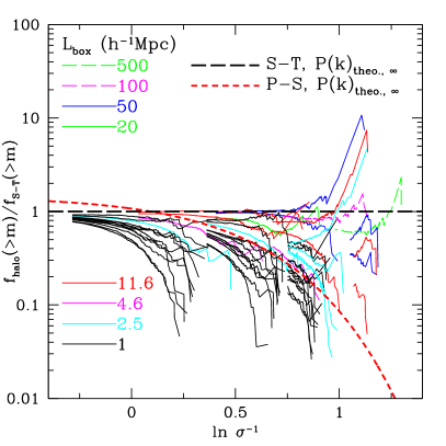
$\begin{array}[]{c@{\hspace{0.2\textwidth}}c}\mbox{\bf(a) Raw simulation mass function}\hfil\hskip 86.72267pt&\mbox{\bf(b) Global mass function}\end{array}$

Figure 3: Cumulative fraction of mass contained in FOF haloes. Left panel assumes ${\rm\sigma_{\infty}(m)}$ (Eqn.. 1), the variance for an infinite universe). Right panel utilises ${\rm\sigma_{sim}(m)}$ (Eqn. 8), the variance-mass relation derived from the mass power spectrum of the initial particle distribution. Accounting for missing large-scale power in this way results in the systematic upward shift in the corrected mass function. Reduced run-to-run scatter and improved agreement between different box sizes (different colours) indicates the effectiveness of the finite volume correction to the mass function.

4.2 Fitting the mass function

An analytic form for the mass function is an essential ingredient for a wide array of models of galaxy formation, reionization, and other phenomena, and is also required for cosmological studies based on observable objects whose number density depends on the halo mass function. In Fig. 4, we show our data along with several analytic functional fits; see also Fig. 5a-d, where we plot the mass function split by redshift. The error bars in Figs. 4-6 are obtained by computing the square root of the number of haloes in each mass bin of a given simulation (see Appendix B for further discussion of uncertainty estimates).

The S-T function provides a reasonable fit except for rare haloes (large $\delta_{c}/\sigma(m,z)$), where the simulations produce $\sim$50$\%$ fewer objects. The P-S function is a poor fit at all redshifts. Of the previously published fits, Reed et al. (2003) is the most consistent with our combined high and low redshift data, fitting the data with an rms difference of 11$\%$, i.e. $\chi^{2}=1$ if we artificially set the uncertainties to be equal to the Poisson errors plus 11$\%$ of the measured abundance, added in quadrature. The Jenkins et al. function is an excellent fit to our low redshift simulation data, but it matches the high redshift data less well. This comparison, however, requires extrapolating the function beyond its intended range of validity, namely the original fitted range of $-1.2<\ln\sigma^{-1}<1.05$. The Warren et al. (2006) curve, which is very similar to the Jenkins et al. form over its original fitted range, fits our lowest redshift data quite well, but it is not as good a fit to our high redshift results.

We now consider whether our data support an improved fit compared to published analytic mass functions. We define the effective slope, $n_{\rm eff}$, as the spectral slope at the scale of the halo, where $P(k_{h})\propto k_{h}^{n_{\rm eff}}$ and $k_{h}=2\pi/r_{0}$, with $r_{0}$ the radius that would contain the mass of the halo at the mean cosmic density. If we limit the fit to a redshift independent form, with the assumption of no dependence on $n_{\rm eff}$, our simulation data can be fit by steepening the high mass slope of the S-T function (Eq. 5) with the addition of a new parameter, $c=1.08$, in the exponential term, and simultaneously including a Gaussian in $\ln\sigma^{-1}$ centred at $\ln\sigma^{-1}=0.4$, as described by the following function, which is otherwise identical to the S-T fit:

$$f(\sigma)=A\sqrt{{2a\over\pi}}\bigg{[}1+\big{(}{\sigma^{2}\over a\delta_{c}^{2}}\big{)}^{p}+0.2G_{1}\bigg{]}{\delta_{c}\over\sigma}\exp\bigg{[}-{ca\delta_{c}^{2}\over 2\sigma^{2}}\bigg{]}$$ (9)

$$G_{1}=\exp\bigg{[}-{{[\ln(\sigma^{-1})-0.4]^{2}}\over{2(0.6)^{2}}}\bigg{]}.$$

For analytical modelling purposes, it is useful to recast this equation in terms of a new variable $\omega^{2}=ca\delta_{c}^{2}/\sigma^{2}$

$$f(\sigma)=A^{\prime}\omega\sqrt{{2\over\pi}}\bigg{[}1+1.02\omega^{2p}+0.2G_{1}\bigg{]}\exp\bigg{[}-{\omega\over 2}\bigg{]}~{}~{}$$ (10)

$$G_{1}=\exp\bigg{[}-{{[\ln({\omega})-0.788]^{2}}\over{2(0.6)^{2}}}\bigg{]},$$

where $A^{\prime}=0.310$ and $ca=0.764$. The resulting function is comparable to the Reed et al. (2003) fit, and is generally consistent with the Sheth & Tormen 2002 modification to the S-T function with a$=$0.75 instead of a$=$0.707 (not plotted). Note that this modification means that the original normalisation criteria – that all mass be contained in haloes, (Eqn. 2) – is not satisfied exactly; instead, 98$\%$ of mass is contained in haloes. It is remarkable that our data at all redshifts over a vast range in masses are generally consistent with a single functional fit that is solely a function of the variance, independent of redshift. However, while this redshift independent function appears reasonable at high redshift, it is relatively poor at $z=0$.

Figure 4: Differential global (corrected for finite volume; see text) mass function of friends-of-friends dark matter haloes for redshift 0, 1, 4, 10, 20, and 30 compared with analytic fits. Thick curves correspond to the modified S-T function (Eq. 10). Error bars denote 1-$\sigma$ poisson uncertainties.

Careful inspection reveals tentative evidence for a dependence on some additional free parameter(s). The mass function at $z\geq 10$ is suppressed, at levels of $\lower 2.15277pt\hbox{\mbox{$\;\buildrel>\over{\sim}\;$}}10-20\%$, relative to lower redshifts, indicating a weak dependence of the mass function on redshift. However, since a given value of $\sigma$ corresponds to different masses at different redshifts, it is unclear whether the apparent trend with redshift masks a dependence on mass or on some other parameter. Regardless of the cause, inclusion of an additional parameter in the mass function provides a better fit to our data, as we now show. We consider the possibility that the mass function may be affected by $n_{\rm eff}$, the power spectral slope at the scale of the halo radius. An improved fit can be made at each redshift with the introduction of $n_{\rm eff}$ in the analytic function, as given by the following formula, again a modification to the S-T function:

$$f(\sigma,n_{\rm eff})=A\sqrt{{2a\over\pi}}\bigg{[}1+\big{(}{\sigma^{2}\over a\delta_{c}^{2}}\big{)}^{p}+0.6G_{1}+0.4G_{2}\bigg{]}$$ (11)

$$\times{\delta_{c}\over\sigma}\exp\bigg{[}-{ca\delta_{c}^{2}\over 2\sigma^{2}}-{0.03\over(n_{\rm eff}+3)^{2}}\big{(}{\delta_{c}\over\sigma}\big{)}^{0.6}\bigg{]},$$

$$G_{1}=\exp\bigg{[}-{{(\ln\sigma^{-1}-0.4)^{2}}\over{2(0.6)^{2}}}\bigg{]},$$

$$G_{2}=\exp\bigg{[}-{{(\ln\sigma^{-1}-0.75)^{2}}\over{2(0.2)^{2}}}\bigg{]}$$

where $c=1.08$, and $G_{1}$ and $G_{2}$ are gaussian functions in $\ln\sigma^{-1}$. This can be rewritten for the purpose of more convenient modelling as

$$f(\sigma,n_{\rm eff})=\bigg{[}1+1.02\omega^{2p}+0.6G_{1}+0.4G_{2}\bigg{]}$$ (12)

$$\times A^{\prime}\omega\sqrt{2\over\pi}\exp\bigg{[}-{\omega\over 2}-{0.0325\omega^{p}\over(n_{\rm eff}+3)^{2}}\bigg{]},$$

$$G_{1}=\exp\bigg{[}-{{[\ln({\omega})-0.788]^{2}}\over{2(0.6)^{2}}}\bigg{]},$$

$$G_{2}=\exp\bigg{[}-{{[\ln({\omega})-1.138]^{2}}\over{2(0.2)^{2}}}\bigg{]},$$

where $A^{\prime}=0.310$ and $ca=0.764$. This function fits the data to 4$\%$ rms accuracy, significantly better than the 15$\%$ rms accuracy of the single parameter fit of Eqn. 10.

The new analytic mass function is presented for redshifts zero through thirty in Fig. 5a-d. The broad “bump” over the S-T function in the $z=0$ mass function centred near $\ln\sigma^{-1}=0.4$, which is also present in the Jenkins et al. and Warren et al. fits, is produced by the Gaussian functions in $\ln\sigma^{-1}$ space. The $n_{\rm eff}$ term introduces a redshift dependence that increasingly suppresses the mass function as $n_{\rm eff}$ approaches -3, and becomes stronger for rarer haloes. From Eqn. 1, it is easy to show that for a pure power-law fluctuation power spectrum, $\sigma^{2}~{}\alpha~{}M^{-(n_{\rm eff}+3)/3}$, which can be reparameterized as

$$n_{\rm eff}=6{{\rm d}\ln\sigma^{-1}\over{\rm d}\ln M\phantom{+}}-3.$$ (13)

At fixed redshift, $n_{\rm eff}$ is thus a proxy for halo mass. At the smallest scales, the CDM power spectrum asymptotes to $n_{\rm eff}=-3$ for a primordial spectral slope $n_{s}=1$ We have computed $n_{\rm eff}$ using Eqn. 13 throughout this paper. However, for convenience, since $n_{\rm eff}$ is nearly linear with $\ln\sigma^{-1}$ over relatively small ranges in $M$, $n_{\rm eff}$ can be approximated to better than $10\%$ in ($n_{\rm eff}+3$) by the following function within the mass and redshift range of haloes in this paper and for $\sigma_{8}=0.9$:

$$n_{\rm eff} \simeq m_{z}\ln\sigma^{-1}+r_{z}$$ (14)

$$m_{z} = 0.55-0.32\bigg{[}1-\big{(}{1\over 1+z}\big{)}\bigg{]}^{5}$$

$$r_{z} = -1.74-0.8\bigg{|}\log\big{(}{1\over 1+z}\big{)}\bigg{|}^{0.8}.$$

In Fig. 6, we plot the ratio of the simulation data to the new analytic fits, with (panel b) and without (panel a) the $n_{\rm eff}$ dependence. The better fit obtained when $n_{\rm eff}$ is included suggests that the halo mass function is not redshift independent and thus cannot be described solely by the single parameter $\sigma(m,z)$. However, panel a) shows that any dependency on additional parameters is very weak. Nevertheless, the precise causes of this apparent dependency warrant further study. Interestingly, the form of $n_{\rm eff}$ dependence modelled in peaks theory (e.g. Sheth 2001) predicts a smaller difference between the numbers of high redshift and low redshift haloes than we find in our simulations.

$\begin{array}[]{c@{\hspace{0.4\textwidth}}c}\mbox{\bf(a) z$\leq$4}\hfil\hskip 173.44534pt&\mbox{\bf(b) z$=$10}\end{array}$

$\begin{array}[]{c@{\hspace{0.4\textwidth}}c}\mbox{\bf(c) z$=$20}\hfil\hskip 173.44534pt&\mbox{\bf(d) z$=$30}\end{array}$

Figure 5: Differential global (corrected for finite volume; see text) mass function of friends-of-friends dark matter haloes for redshift 10, 20, and 30 compared with analytic fits, including our new two-parameter fit (Eqn. 11), which includes a dependence on spectral slope, $n_{\rm eff}$, and the resulting redshift dependence.

$\begin{array}[]{c@{\hspace{0.4\textwidth}}c}\mbox{\bf(a) $f(\sigma)$}\hfil\hskip 173.44534pt&\mbox{\bf(b) $f(\sigma,n_{\rm eff})$}\end{array}$

Figure 6: Ratio between the differential global (corrected for finite volume; see text) mass function of friends-of-friends dark matter haloes at redshift 0, 1, 4, 10, 20 and 30, and our single parameter fit (left; Eqn. 10); ratio between the same simulation data and a new fit that includes $n_{\rm eff}$ as a second parameter (right; Eqn. 11). The improved fit in the right panel shows that our results are better described by a two-parameter function, rather than simply a function of $\ln\sigma^{-1}$. This is evidence for a weak redshift dependence (via $n_{\rm eff}$) of the mass function.

5 sensitivity to cosmological parameters

Our general results are unaffected by the exact values of the cosmological parameters because the fit of the mass function in the simulations to an analytic form is, in principle, independent of the precise relation between variance and mass (although a dependence on $n_{\rm eff}$ introduces a weak dependence on cosmological parameters through the relation between $n_{\rm eff}$ and $\sigma(m,z)$). Studies involving a wide range of cosmological parameters (e.g. Jenkins et al. 2001; White 2002) have ruled out a strong dependence of f($\sigma$) on matter or energy density. This allows one to estimate the halo abundance for a range of plausible cosmological parameters using purely the analytic mass function determined by $\sigma(m,z)$. In particular, the third year WMAP results (WMAP-3), which confirm the analysis by Sanchez et al. (2006) of the first year WMAP and other CMB experiments combined with the 2dFGRS, imply a fluctuation amplitude significantly smaller than is commonly assumed, and also suggest a spectral index smaller than 1. Both of these parameters have a significant impact on the number of small haloes at high redshift.

Figs. 7 and 8 show that, compared to the cosmology assumed in the rest of this paper ($\sigma_{8}=0.9$, $n_{s}=1.0$, $\Omega_{m}=0.25$), the cosmological parameters inferred from the WMAP-3 data imply a factor of 5 decrease in the number of candidate galaxy hosts at $z=10$ with mass $\sim 10^{8}$ $h^{-1}{\rm{M}}_{\odot}$, and more than four orders of magnitude decrease in the number of potential galaxies at $z=30$ with mass $\sim 2\times 10^{7}$ $h^{-1}{\rm{M}}_{\odot}$ . Smaller “mini-haloes” which could host population III stars are also strongly affected. The WMAP-3 cosmology implies less than half the number of “mini-haloes” of mass $\sim 10^{6}$ $h^{-1}{\rm{M}}_{\odot}$ at $z=10$ and a reduction by more than three orders of magnitude at $z=30$ relative to our standard cosmology. Note that the comoving abundances in Fig. 7 do not match exactly the values in Fig. 1 because a slightly different transfer function was used for some of the simulations, as discussed in §2.1.

The effect of the WMAP-3 cosmological parameters can also be interpreted either as reducing the mass of typical haloes at a given redshift, or as introducing a delay in the formation of structure. For example, haloes with number density $1~{}h^{3}$Mpc^-3 at $z=10$ would have a mass approximately four times larger in our standard cosmology than in the WMAP-3 cosmology; for the same fixed number density, this becomes a factor of $\sim$10 at $z=20$ and a factor of $\sim$25 at $z=30$. For haloes of a fixed mass, the reduced $\sigma_{8}$ and $n_{s}$ of the WMAP-3 cosmology delay halo formation. For example, haloes of mass of $10^{8}h^{-1}{\rm{M}}_{\odot}$ are delayed by $\Delta~{}z\simeq 6$ (z$=$21 to z$=$15) before reaching a comoving abundance of $10^{-2}~{}h^{3}$Mpc^-3. Haloes of $10^{6}h^{-1}{\rm{M}}_{\odot}$, approximately the mass where H₂-cooling becomes strong enough to trigger star formation, do not reach an abundance of $1~{}h^{3}$Mpc^-3 until $z=21$ for the WMAP-3 cosmology compared to $z=30$ for our standard cosmology. This means that widespread population III star formation and galaxy formation would occur significantly later if the WMAP-3 cosmological parameters were correct.

The uncertainties that remain in the values of cosmological parameters translate into significant uncertainties in the number of high redshift haloes that can potentially host luminous objects, especially those haloes that host the first generations of stars and galaxies. This adds major uncertainty to predictions of the abundance of potentially detectable haloes in the pre-reionized universe, such as those modelled in e.g. Reed et al. (2005). However, the sensitivity of halo number density to cosmological parameters suggests the exciting prospect of using the number of small haloes at high redshift as a cosmological probe if future studies are able to establish their number density accurately. Such measurements of high redshift halo numbers would require not only extremely sensitive observations, but also further theoretical work to better understand the relation between observable properties and halo mass.

Figure 7: Differential analytic mass function for the WMAP 3-year cosmological parameters (Spergel et al. 2006), compared with the mass function for the standard cosmological parameters assumed in the simulations of this work. The curves marked “WMAP 3yr” use the preferred WMAP 3-year parameters (e.g. $\sigma_{8},n_{s}=0.74,0.951$), including the effect of the preferred parameters(e.g. $\Omega_{m}$, $\Omega_{baryon}$, etc) on the transfer function. The abundance of massive, high redshift haloes is highly sensitive to cosmological parameters due to the steepness of the mass function.

Figure 8: Cumulative abundance versus redshift for the WMAP 3-year cosmological parameters (Spergel et al. 2006) implied by our new analytic mass function (Eqn. 11). Also shown is the abundance of haloes for the standard cosmological parameters assumed in the simulations of this work for 3 masses. The curves are labelled by mass in units of $h^{-1}{\rm{M}}_{\odot}$. The curves marked “WMAP 3yr” assume the complete preferred WMAP 3-year parameters ($\sigma_{8},n_{s}=0.74,0.951$), including the effect of the preferred parameters (e.g. $\Omega_{m}$, $\Omega_{baryon}$, etc) on the transfer function. The abundances at high redshift are most sensitive to cosmological parameters.

6 discussion

Our simulations give the mass function of dark matter haloes out to redshift 30 and down to masses that include the smallest haloes likely to form stars, “mini-haloes” whose baryons collapse through H₂ cooling. Thus, we now have a precise estimate of the mass function of the haloes that contain all the stellar material at observable redshifts, and at virtually all the redshifts that are potentially observable in the foreseeable future. Our fits were obtained using simulations of the $\Lambda$CDM cosmology for a specific set of cosmological parameters, but they are readily scalable to other values.

These haloes may be detected in a numbers of ways. Large haloes (those with T${}_{\rm vir}>10^{4}$K), which have the potential to host galaxies formed by efficient baryon cooling, might be observed out to the epoch of reionization with the JW Space Telescope, or perhaps even with current generation infrared observatories. Smaller haloes may not be directly observable. However, their stellar end-products might, as gamma-ray bursts (e.g. Gou et al. 2004), or as supernovae at redshifts well above the epoch of reionization (e.g. Weinmann & Lilly 2005).

Knowledge of the halo mass function will be important in the interpretation of data from the Low Frequency Array (LOFAR), the Square Kilometer Array (SKA) or other rest-frame 21cm experiments designed to discover and probe the epoch of reionization. It may even be possible to use the halo mass function to help break degeneracies between cosmological parameters and the astrophysical modelling of the first objects.

Our results for the halo mass function at high redshift imply that predictions for the abundance of dark matter haloes that may host galaxies, stars, gamma-ray bursts or other phenomena based on the commonly used Press-Schechter model grossly underestimate the number of 3 $\sigma$ or rarer haloes. This includes large galaxies at $z\sim 10$, all haloes large enough to host galaxies at $z\lower 2.15277pt\hbox{\mbox{$\;\buildrel>\over{\sim}\;$}}15$, and all haloes capable of hosting stars at $z\lower 2.15277pt\hbox{\mbox{$\;\buildrel>\over{\sim}\;$}}20$, assuming that a halo must be at least $\sim 10^{8}$ $h^{-1}{\rm{M}}_{\odot}$ to host a galaxy and $10^{6}$$h^{-1}{\rm{M}}_{\odot}$ to form stars. The P-S function underestimates the true mass function by a factor $\sim 5$ for the rarest haloes that we have simulated, which applies to galaxy candidates at $z=30$, and large ($\sim 10^{11}h^{-1}{\rm{M}}_{\odot}$) galaxies at $z=10$. The abundance of mini-haloes likely to host Population III stars are underestimated by the P-S function by a factor of at least two at $z=30$. Studies that assume the Sheth & Tormen function are more robust, but they still suffer from an overestimation of the numbers of large haloes at high redshift, particularly of large galaxies at $z\lower 2.15277pt\hbox{\mbox{$\;\buildrel>\over{\sim}\;$}}10$, extending to all potential galaxies at $z\lower 2.15277pt\hbox{\mbox{$\;\buildrel>\over{\sim}\;$}}20$, and to all star-forming haloes at $z\lower 2.15277pt\hbox{\mbox{$\;\buildrel>\over{\sim}\;$}}30$, reaching a factor of up to $\sim$3 for the rarest haloes in our simulations. However, the S-T function overpredicts the number of mini-haloes only by less than $\sim 20\%$ at $\;\buildrel<\over{\sim}\;$20 and by $\sim 40\%$ at $z=30$.

7 summary

We have determined the mass function of haloes capable of sustaining star formation from redshift 10 to 30, a period beginning well before reionization and extending to redshifts below those where reionization occurred according to the WMAP 3-year estimates. This extends the mass function to lower masses and higher redshifts than previous work, and includes the “mini-haloes” that probably hosted population III stars. Our main results may be summarised as follows:

$\bullet$ We have presented a novel method for correcting for the effects of cosmic variance and unrepresented large-scale power in finite simulation volumes. This allows one to infer more accurately the true global mass function, ultimately allowing the mass function to be computed to smaller masses. We have verified the robustness of this method by carrying out simulations of a wide range of volumes and mass resolutions and comparing the inferred mass functions for overlapping halo mass ranges. By simulating multiple realisations of identical volumes, we show that the run-to-run scatter in the mass function, caused by cosmic variance, is minimised by our method.

$\bullet$ Throughout the period $10<z<30$, the halo mass function is broadly consistent with the Sheth & Tormen (1999) model for haloes $3\sigma$ and below. For rarer haloes, the mass function drops increasingly below the S-T function – by up to $\sim 50\%$ for $\sim 5\sigma$ haloes.

$\bullet$ Our data are reasonably well fit by a redshift-independent function of $\sigma(m,z)$, the rms linear variance in top hat spheres. We provide a 1-parameter fit to the mass function which is a modified version of the Sheth & Tormen (1999) formula. However, an even better fit can obtained if the mass function is allowed to depend not only on $\sigma(m,z)$, but also on the slope of the primordial mass power spectrum, $n_{\rm eff}$. This improvement implies that that the fraction of collapsed mass does not depend solely on the rms linear overdensity, as is assumed in Press-Schechter theory. The P-S formula, in fact, provides a poor fit to must of our data.

$\bullet$ The halo abundance at $z\lower 2.15277pt\hbox{\mbox{$\;\buildrel>\over{\sim}\;$}}10$ is highly sensitive to $\sigma_{8}$ and $n_{s}$, parameters recently adjusted downwards in the reported WMAP 3-year results (Spergel et al. 2006). The new estimates imply greatly reduced numbers of high redshift haloes of a given mass. The sensitivity of high-redshift halo numbers to these parameters suggests their potential as a useful cosmological probe in future.

Code to generate our best-fit halo mass function may be downloaded from http://icc.dur.ac.uk/Research/PublicDownloads/genmf_readme.html

Appendix A numerical tests

A.1 Run parameter convergence tests

In Fig. 9, we have tested some of the primary runtime parameters of L-Gadget2 using a $10^{3}$$h^{-1}{\rm{M}}_{\odot}$ particle resolution 1 $h^{-1}$Mpc volume. These tests confirm that our choices of starting redshift (${\rm z_{start}}$), fractional force accuracy (${\rm\Delta_{force~{}acc}=0.005}$), softening length (${\rm r_{soft}}$), and maximum allowed timestep ($\Delta_{t}=\Delta\ln(1+z)^{-1}$) are sufficient. Of the parameters that we have tested, ${\rm z_{start}}$ has the most effect on our results. At z$=$10, ${\rm z_{start}}=119$ is indistinguishable from earlier starting redshifts. However, at z$=$20, the ${\rm z_{start}}=119$ mass function is suppressed by $\sim 10-20\%$ relative to the ${\rm z_{start}}=299$ runs, and by more than $50\%$ at z$=$30. At z$=$30, the ${\rm z_{start}}=299$ run is suppressed relative to the ${\rm z_{start}}=599$ run by $\sim 10-20\%$, which could indicate a small bias in our z$=$30 mass function, but not large enough to affect significantly our conclusions. It thus appears that a simulation must be evolved a factor of $\sim$10 in expansion factor in order to solve accurately (within 10-20$\%$) the mass function for the mass resolutions and outputs we have considered, if one uses the Zel’dovich (1970) approximation to set up initial conditions, as we have. Note that the convergence of our runs with increased starting redshift implies that the Zel’dovich approximation is valid. See discussion in following section.

$\begin{array}[]{c@{\hspace{0.25\textwidth}}c@{\hspace{0.25\textwidth}}c}\mbox{\bf(a) z$=$10}\hfil\hskip 108.405pt&\mbox{\bf(b) z$=$20}\hfil\hskip 108.405pt&\mbox{\bf(c) z$=$30}\end{array}$

Figure 9: Differential raw (unadjusted for finite volumes) simulated mass function of friends-of-friends dark matter haloes for redshifts 10, 20, and 30 is shown for several run parameters. Unless otherwise noted, each run used the parameters implemented throughout this paper (${\rm z_{start}=119}$, ${\rm\Delta_{force~{}acc}=0.005}$, ${\rm r_{soft}=l_{mean}/20}$, $\Delta_{t}=0.02$) , except that the green (${\rm\Delta_{force~{}acc}}$), and magenta (r_soft) curves used ${\rm z_{start}=119}$. Here haloes are plotted down to 20 particles per halo versus the 100 particle minimum imposed throughout the paper; particle mass is $1.1\times 10^{3}h^{-1}{\rm{M}}_{\odot}$.

A.2 Resolving haloes

Studies of the mass function at low redshift have found that the mass function is adequately sampled for haloes containing as few as 20 particles (e.g. Jenkins et al. 2001). Because we are exploring new regimes in mass and redshift, it is necessary to confirm that we model haloes with sufficient particle numbers to resolve the mass function. The FOF mass function for haloes of very few particles is typically enhanced artificially as spurious groupings are increasingly common for small particle numbers.

Our resolution tests consists of an identical volume, simulated at multiple mass resolutions. The mass function of a 2.5 $h^{-1}$Mpc box at resolutions of 200³, 500³, and 1000³ is shown in Figure 10. At each resolution, the mass function has an upturn below approximately 30-40 particles. Additionally, the mass function is suppressed over the range of $\sim$30 to $\sim$100 particles, at a level that appears to depend on redshift. At scales larger than approximately 100 particles, the mass function at multiple resolutions agrees within the uncertainties. For this reason, we limit our analysis to haloes of at least 100 particles. This resolution limit is significantly higher than found necessary at low redshift in many previous works. Even with this conservative particle resolution limit, some small bias in the mass function cannot be ruled out fully for redshifts 20 or higher. The increased sensitivity of the mass function to particle resolution as redshift increases is likely enhanced by the increased steepness of the mass function in this regime for haloes formed from rare fluctuations. The suppression of the mass function for haloes of fewer than 100 particles may be due to transient effects that become unimportant by lower redshifts. These effects could include errors introduced as a result of inaccuracies of the Zel’dovich approximation (Zel’dovich 1970) where initial particle positions and velocities are computed based on the initial density field, which is assumed to be entirely linear. If so, then these transients could be reduced by using second order Lagrangian perturbation theory (2LPT; Scoccimarro 1998, Crocce, Pueblas & Scoccimarro 2006) to set up initial conditions. Use of 2LPT may also reduce the required starting redshift. Further investigation is required to determine more fully the sources of increased sensitivity to mass resolution on the mass function.

Figure 10: Residuals of the differential raw (unadjusted for finite volumes) mass function for a 2.5 $h^{-1}$Mpc box with identical initial density fluctuations modelled at 3 different mass resolutions (200³, 500³, and 1000³ particles). Thick line segments denote haloes of at least 100 particles, the minimum particle number that we implement throughout the paper. Thin line segments show the mass function down to 20 particles per halo.

A.3 Halo finders: friends-of-friends (FOF) versus spherical overdensity (SO)

Choice of halo finder can have a major impact on halo masses and on the mass function. It is thus worth considering how our results would change had we used a different halo finder. In this case, the FOF mass function is compared with the mass function produced by the spherical overdensity SO algorithm (Lacey & Cole 1994), which identifies spheres of a specified overdensity. FOF is computationally efficient and will select objects of any shape provided that they meet a local particle density. However, FOF may also spuriously link together neighbouring haloes, which is a potential issue for low mass, high redshift haloes which form at scales where mass fluctuation spectrum is steep, and result in highly ellipsoidal halo shapes (Gao et al. 2005). Because SO assumes haloes are spheres, it is not ideal for highly ellipsoidal haloes. However, SO has an advantage over FOF in that it is less likely spuriously to link together neighbouring haloes or to misclassify highly ellipsoidal but unvirialized structures as haloes.

We have tested the SO algorithm assuming the spherical tophat model, in which the $\Lambda$CDM virial overdensity, $\Delta_{\rm vir}$, in units of the mean density is 178 at high redshifts, when $\Omega_{m}\simeq 1$. We have computed the SO mass function for three simulations of particle mass resolution $\sim$ 10³, 10⁵, and 10⁷ $h^{-1}{\rm{M}}_{\odot}$ at redshifts 10, 20, and 30. In Figure 11, we show the SO and FOF mass functions for these outputs. In general, the SO mass function is lower than the FOF mass function, though the two mass functions are consistent for much of the redshift 10 mass range. The difference between the two mass functions increases with mass and redshift, ranging from $\;\buildrel<\over{\sim}\;$10$\%$ at redshift 10 and is generally less than a factor of 2. Some caution should be taken when considering the SO mass function because of its particle number dependence in this implementation of the SO halo finder. Initial candidate centres for SO haloes were identified by finding density peaks, where local density was computed for each particle, smoothed by its 32 nearest neighbours. Spheres were then grown outward until the desired overdensity was reached. This means that SO haloes with masses approaching and below the 32 particle smoothing mass will be suppressed.

While there are some differences in the mass function for the two means of identifying haloes, these differences are generally smaller than the differences introduced by adopting the WMAP 3 year cosmological parameters versus the larger $\sigma_{8}=0.9$ and $n_{s}=1.0$ used in the simulations of this paper.

Figure 11: friends-of-friends (FOF, thin lines) and spherical overdensity (SO, thick lines) halo differential raw (unadjusted for finite volumes) mass functions for particle masses of $\sim$ 10³, 10⁵, and 10⁷ $h^{-1}{\rm{M}}_{\odot}$ (box size of 1.0, 4.6, and 20 $h^{-1}$Mpc with 400³ particles). SO density is 178 times the mean density. Curves are plotted down to 20 particles per halo.

Appendix B uncertainties and run to run scatter

In this section, we discuss uncertainties and run to run variance using the 2.5 $h^{-1}$Mpc and 1 $h^{-1}$Mpc boxes at z$=$10 as examples. Fig. 12-13 shows that the poisson ($\sqrt{n}$) estimate of uncertainty is much smaller than the “bootstrap” uncertainty computed by taking the rms variance between random subsamples. The scatter between 3 non-overlapping subsamples with low overdensity, ($|\delta|<10^{-3}$), is much smaller, and is in fact comparable to the scatter between individual simulations of 1 $h^{-1}$Mpc cubes. Although there are too few low overdensity subvolumes for a truly representative sample, their similarity suggests that most of the variance between the random subvolumes is due to non-zero mean density.

Between the 11 small (1 $h^{-1}$Mpc) simulations, the run to run variance is comparable to their individual average poisson uncertainty. This suggests that poisson uncertainty provides a reasonable estimate of the true uncertainty provided that other finite volume effects, such as missing large scale power, are taken into account (see earlier discussion). The mean mass function for low mass haloes is consistent among these subvolumes and small volume simulations. However, for the low overdensity subvolumes, the mean mass function is deficient in massive haloes.

Figure 12: Comparison of uncertainty estimators using the differential raw (unadjusted for finite volumes) mass functions for particle masses of z$=$10. Filled squares (black) show the 2.5 $h^{-1}$Mpc run with poisson errors (where uncertainty is assumed to be equal to the square root of the number of haloes in each mass bin, as throughout the paper). Large X’s (blue) denote the mean and rms variance of the mass function of 11 random 1 $h^{-1}$Mpc subvolume cubes selected from the same volume. Open circles (cyan) are the mean and rms of 3 low overdensity 1 $h^{-1}$Mpc subvolmes.

Figure 13: Comparison of uncertainty estimators using the differential raw (unadjusted for finite volumes) mass functions for particle masses of z$=$10. Filled squares (black) show the 2.5 $h^{-1}$Mpc run with $\sqrt{n}$ poisson errors. Triangles (magenta) denote the mean mass function of the eleven 1 $h^{-1}$Mpc simulations with poisson uncertainty (magenta error bars) and run to run rms variance (red error bars).

References

- (1) Abel T., Bryan G., Norman M. L., 2000, ApJ, 540, 39
- (2) Abel T., Bryan G., Norman M. L., 2002, Science, 295, 93
- (3) Bagla J., Ray S., 2005, MNRAS, 358, 1076
- (4) Bagla J., Prasad J., 2006, MNRAS, 370, 993
- (5) Barkana R., Loeb A., 2004, ApJ, 609, 474
- (6) Bond J. R., Cole S., Efstathiou G., Kaiser N., 1991, MNRAS, 379, 440
- (7) Bond J., Efstathiou G., 1984, ApJ, 285, 45
- (8) Bower R., 1991, MNRAS, 248, 332
- (9) Bromm V., Coppi P. S., Larson R. R., 1999, ApJ, 527, L5
- (10) Bromm V., Coppi P. S., Larson R. R., 2002, ApJ, 564, 23
- (11) Bromm V., Larson R., 2004, ARA&A, 42, 79
- (12) Ciardi B., Ferrara A., 2005, Space Science Reviews, 116, 625
- (13) Colberg J., et al. , 2000, MNRAS, 319, 209
- (14) Cole S., 1997, MNRAS, 286, 38
- (15) Couchman H., Thomas P., Pearce F., 1995, ApJ, 452, 797
- (16) Crocce M., Pueblas S., Scoccimarro R., 2006, astro-ph/0606505
- (17) Davis, M., Efstathiou, G., Frenk, C.S., White, S.D.M., 1985, ApJ, 292, 381
- (18) Efstathiou G., Davis M., White S. D. M. Frenk C. S., 1985, ApJS, 57, 241
- (19) Efstathiou G., Frenk C. S., White S. D. M., Davis M., 1988, MNRAS, 235, 715
- (20) Eke V., Cole S., Frenk C.S., 1996, MNRAS, 282, 263.
- (21) Gao L., White S. D. M., Jenkins A., Frenk C. S., Springel V., 2005, MNRAS, 363, 379
- (22) Gou L., Mesazaros P., Abel T., Zhang B., 2004, ApJ, 604, 508
- (23) Heitmann K., Lukic Z., Habib S., Ricker P., 2006, ApJ, 624, 85
- (24) Iliev I., Mellema G., Pen U., Shapiro P., Alvarez M., 2006, MNRAS, 369, 1625
- (25) Jang-Condell H., Hernquist L., 2001, ApJ, 548, 68
- (26) Jenkins A., Frenk C. S., White S. D. M., Colberg J., Cole S., Evrard A., Couchman H., Yoshida N., 2001, MNRAS, 321, 372
- (27) Lacey C., Cole S., 1993, MNRAS, 262, 627
- (28) Lacey C., Cole S., 1994, MNRAS, 271, 676
- (29) Linder, E. V., Jenkins, A., 2003, MNRAS, 346, 573
- (30) Lokas, E. L., Bode, P., Hoffmann, Y., MNRAS, 349, 595
- (31) Mo H., White S. D. M., 1996, MNRAS, 282, 347
- (32) Monaco P., Theuns T., Taffoni G., Governato F., Quinn T., Stadel J., 2002, ApJ, 564, 8
- (33) Monaco P., Theuns T., Taffoni G., 2002, MNRAS, 331 587
- (34) Naoz S., Barkana R., 2005, MNRAS, 362, 1047
- (35) Naoz S., Noter S., Barkana R., 2006, astro-ph/0604050
- (36) Pearce F., Couchman H., 1997, NewA, 2, 411
- (37) Peebles P., 1993, Principles of Physical Cosmology, Princeton Univ. Press, Princeton, NJ, USA
- (38) Power C., Knebe A., 2006, MNRAS, 370, 691
- (39) Press W.H., Schechter P., 1974, ApJ, 187, 425
- (40) Reed D., Gardner J., Quinn T., Stadel J., Fardal M., Lake G., Governato F., 2003, MNRAS, 346, 565
- (41) Reed D. S., Bower R., Frenk C.S., Gao L., Jenkins A., Theuns T., White S.D.M., 2005, MNRAS, 363, 393
- (42) Sanchez A., Baugh C., Percival W., Peacock J., Padilla N., Cole S., Frenk C., Norberg P., 2006, MNRAS, 366, 189
- (43) Schneider R., Salvaterra R., Ferrara A., Ciardi B., 2006, MNRAS, 369, 825
- (44) Scoccimarro R., 1998, MNRAS, 299, 1097
- (45) Seljak U., Zaldarriaga M., 1996, ApJ, 469, 437
- (46) Sheth R., 2001, NYAS, 927, p. 1-12
- (47) Sheth R., Tormen G., 1999, MNRAS, 308, 119
- (48) Sheth R., Tormen G., 2002, MNRAS, 329, 61
- (49) Sheth R., Mo H., Tormen G., 2001, MNRAS, 323, 1
- (50) Sirko E., 2005, ApJ, 634, 728
- (51) Spergel D., et al. , 2003, ApJS, 148, 175
- (52) Spergel D., et al. , 2006, astro-ph/0603449
- (53) Springel V., 2005, MNRAS, 364, 1105
- (54) Springel V., et al. , 2005, Nature, 435, 629
- (55) Tormen G., Bertschinger E., 1996, ApJ, 472, 14
- (56) Warren M., Abazajian K., Holz D., Teodoro L., 2006, ApJ, 646, 881
- (57) Weinmann S., Lilly S., 2005, ApJ, 624, 526
- (58) White M., 2002, ApJS, 143, 241
- (59) White S. D. M., Springel V., 2000, “Where are the first starts now?”, The First Stars, Proceedings, eds Weiss A., Abel T., & Hill V., Springer, p. 327
- (60) Yamamoto K., Sigiyama N., Sato H., 1998, ApJ, 501, 442
- (61) Yoshida N., Sugiyama N., Hernquist L., 2003, MNRAS, 344, 481
- (62) Zahn O., Lidz A., McQuinn M., Dutta S., Hernquist L., Zaldarriaga M., Furlanetto S., 2006, astro-ph/0604177
- (63) Zel’dovich Y., 1970, A&A, 5, 84