Survey for Galaxies Associated with $z\sim 3$ Damped Lyman $\alpha$ Systems II: Galaxy-Absorber Correlation Functions

Abstract

We use 211 galaxy spectra from our survey for Lyman break galaxies (LBGs) associated with 11 damped Lyman $\alpha$ systems (DLAs) to measure the three-dimensional LBG auto-correlation and DLA-LBG cross-correlation functions with the primary goal of inferring the mass of DLAs at $z\sim 3$. From every measurement and test in this work, we find evidence for an overdensity of LBGs near DLAs and find this overdensity to be very similar to that of LBGs near other LBGs. Conventional binning of the data while varying both $r_{0}$ and $\gamma$ parameters of the fiducial model of the correlation function $\xi(r)=(r/r_{0})^{-\gamma}$ resulted in the best fit values and $1\sigma$ uncertainties of $r_{0}=2.65\pm 0.48,\gamma=1.55\pm 0.40$ for the LBG auto-correlation and $r_{0}=3.32\pm 1.25,\gamma=1.74\pm 0.36$ for DLA-LBG cross-correlation function. To circumvent shortcomings found in binning small datasets, we perform a maximum likelihood analysis based on Poisson statistics. The best fit values and $1\sigma$ confidence levels from this analysis were found to be $r_{0}=2.91^{+1.0}_{-1.0},~{}\gamma=1.21^{+0.6}_{-0.3}$ for the LBG auto-correlation and $r_{0}=2.81^{+1.4}_{-2.0}$, $\gamma=2.11^{+1.3}_{-1.4}$ for the DLA-LBG cross-correlation function. We report a redshift spike of five LBGs with $Deltaz=0.015$ of the $z=2.936$ DLA in the PSS0808+5215 field and find that the DLA-LBG clustering signal survives when omitting this field from the analysis. Using the correlation functions measurements and uncertainties, we compute the $z\sim 3$ LBG galaxy bias $b_{LBG}$ to be $1.5<b_{LBG}<3$ corresponding to an average halo mass of $10^{9.7}<\langle M_{LBG}\rangle<10^{11.6}~{}M_{\odot}$ and the $z\sim 3$ DLA galaxy bias $b_{DLA}$ to be $1.3<b_{DLA}<4$ corresponding to an average halo mass of $10^{9}<\langle M_{LBG}\rangle<10^{12}~{}M_{\odot}$. Lastly, two of the six QSOs discovered in this survey were found to lie within $\Delta z=0.0125$ of two of the survey DLAs. We estimate the probability of this occurring by chance is 1 in 940 and may indicate a possible relationship between the distribution of QSOs and DLAs at $z\sim 3$.

1 Introduction

One of the most fundamental measurements of high redshift galaxies is their spatial distribution, largely because this information can be used to infer their average dark matter halo mass. Standard CDM cosmology details the process in which galaxies formed by the gravitational collapse of primordial dark matter density fluctuations. In the early universe, low-mass fluctuations typically had density contrasts high enough to collapse against the Hubble flow and formed uniformly throughout space whereas high-mass fluctuations with high density contrasts were rare. However, the superposition of density fluctuations resulted in the collapse of an excess number of high-mass fluctuations clustered near the peaks of underlying mass overdensities that sufficiently enhanced their density contrast. It is in this context that the measurement of the clustering of galaxies infers the underlying dark matter halo mass of these systems.

Several surveys over the last decade have been used to infer the dark matter mass of high redshift galaxy populations by their angular clustering [e.g., Daddi et al. (2000, 2004); McCarthy et al. (2001, 2004); Porciani & Giavalisco (2002); Foucaud et al. (2003)]. One population, the Lyman break galaxies (LBGs), are identified photometrically by the decrement (break) in their continua shortward of the Lyman limit caused by absorption from optically thick intervening systems in the line-of-sight. The spectroscopic survey of Steidel et al. (1998) provided sufficient spectra for a measurement of the three-dimensional distribution of LBGs at $z\sim 3$. Analysis of that data by Adelberger et al. (1998) showed evidence of significant clustering corresponding to halo masses of $\sim 10^{11-12}M_{\odot}$. The faint emission from LBGs restricts observations to low signal-to-noise ratio low-resolution spectra using current technology. As a consequence, the properties of this magnitude limited sample must be examined statistically and/or from composite spectra. In addition, the selection methods employed to detect LBGs are not sensitive to all types of galaxies at high redshift and therefore partially incomplete.

Quasar absorption-line systems provide a complementary means to study high redshift systems. Their detection is dependent only on the brightness of the background source and the strength of the absorption-line features and is not biased by intrinsic magnitudes or photometric selection criteria. A subset of this population, the damped Lyman $\alpha$ systems (DLAs), are defined to have column densities of N(Hi) $>2\times 10^{20}$ atoms cm^-1 (Wolfe et al., 1986, 2005) and contain $\sim 80\%$ of the Hi content of the universe (Prochaska, Herbert-Fort, & Wolfe, 2005). DLAs have column densities high enough to provide self-shielding against ambient ionizing radiation and thereby protect large reservoirs of neutral gas. Several lines of evidence, including high-resolution analysis of DLA gas kinematics (Prochaska & Wolfe, 1997, 1998; Wolfe & Prochaska, 2000a, b) and the agreement between the comoving neutral gas density at $z>2$ and the mass density of visible stars in local disks (Wolfe et al., 1995), have fueled the belief that DLAs are capable of evolving into present-day galaxies like the Milky Way (Kauffmann, 1996).

It becomes clear that studies of galaxy formation are incomplete without understanding the population of proto-galaxies that DLAs represent. Although properties such as the gas kinematics and chemical abundances of DLAs can be studied with high resolution and are well documented, the mass of these systems has remained unknown. The sparse distribution of DLAs in QSO sight-lines prohibits the use of their clustering as a tracer of the underlying dark matter mass. Instead, the host halo mass of DLAs can be inferred by their cross-correlation with another known population. In this work, we utilize the ubiquitous LBGs at $z\sim 3$ for this purpose. This paper is the second in a series (Cooke et al. (2005), hereafter Paper I) reporting the results of a survey of LBGs detected near 11 DLAs at $z\sim 3$ with the primary goal of inferring the mass of DLAs from the DLA-LBG spatial cross-correlation.

This paper is organized as follows: We briefly review the imaging and spectroscopic observations in §2, present spectra of the objects detected near the DLAs in §3 and the spectra of the faint AGN discovered in the survey in §4. We describe the methodology behind the clustering analysis in §5 and present the LBG auto-correlation and DLA-LBG cross-correlation results by technique, including tests of these results, in §6. We discuss the implications on the galaxy bias and mass of DLAs in §7, provide a brief discussion in §8 and a summary of the survey in §9. We adopt $\Omega_{M}$=0.3, $\Omega_{\Lambda}$=0.7, $h=100$ cosmology unless otherwise noted, primarily for direct comparison to the literature. All correlation lengths $r_{0}$ reported in this work are in $h^{-1}$Mpc comoving.

2 Survey Design

Our first goal was to efficiently select LBGs at $z\sim 3$ via their photometric colors. To achieve this, we developed a $u^{\prime}$ BVRI photometric selection technique, primarily due to filter availability, that fulfilled the imaging goals and resulted in an efficacy very similar to previous work. Our second observational goal was the accurate acquisition and analysis of a few hundred faint $z\sim 3$ galaxy spectra. This was accomplished using the Keck telescope and low-resolution multi-object spectroscopy. A detailed description of the data acquisition, reduction and analysis and comparison to previous $U_{n}G\cal{R}$I surveys can be found in Paper I. Here, we discuss a few relevant points of the observations.

2.1 The DLA Sample

The QSO fields targeted in this survey were selected from the subset that met the following constraints: (1) The QSO was required to display at least one known DLA in the redshift range where our $u^{\prime}$BVRI photometric selection is most effective ($2.6<z<3.4$), (2) systems within 3000 km s^-1 from the background QSO were not used to avoid proximity effects and, (3) a preference was given to fields that would be observed through the lowest airmass and in the direction of lowest Galactic reddening to minimize the flux attenuation of $z\sim 3$ sources. Table 1 lists our survey fields. At the time this survey began, only $\sim 30$ DLAs met these criteria. From this subset, the targets were chosen at random. The mean column density of the 11 DLAs in this survey is log N(Hi) $=20.94$ atoms cm^-2 with a typical individual error of $\pm 0.1$, whereas the mean DLA column density measured recently from 197 DLAs taken over the same redshift range from the SDSS survey (Prochaska, Herbert-Fort, & Wolfe, 2005) is N(Hi) $=20.84$ atoms cm^-2 and a typical error of $\pm 0.2$. Therefore, the DLAs presented here appear to be a good representation of $z\sim 3$ DLAs on average.

2.2 Imaging

We obtained deep $u^{\prime}$BVRI imaging of nine QSO fields with 11 known $z\sim 3$ DLAs from 2000 April to 2003 November using the Low-Resolution Imager and Spectrometer (LRIS; Oke et al., 1995) on the 10m Keck I telescope and the Carnegie Observatories Spectrograph and Multi-object Imaging Camera (COSMIC; Kells et al., 1998) on the 5m Hale telescope at the Palomar Observatory. Object placement and image field size are topics that deserve a brief discussion. The DLAs were approximately centered in the images in which seven have a field of view of $\sim 6^{\prime}\times 7.5^{\prime}$ (LRIS) and two have a field of view $\sim 9.7^{\prime}\times 9.7^{\prime}$ (COSMIC). The usable area of each of the final stacked images was reduced in both dimensions by $\lesssim 40"$ from our imposed dithering sequence. This resulted in maximum (diagonal) comoving object separations of $\sim 10h^{-1}$Mpc (LRIS) and $\sim 13h^{-1}$Mpc (COSMIC) at $z\sim 3$ and about half this distance for the DLAs. The correlation length of LBGs at $z\sim 3$ has been measured to be $3.96\pm 0.29h^{-1}$Mpc by Adelberger et al. (2003), hereafter A03. As a result, the angular clustering component in our survey cannot be measured much beyond $1-2$ correlation lengths, yet the redshift path of $\sim 540h^{-1}$Mpc, where our photometric selection is best described ($2.6<z<3.4$), allows complete analysis of the distribution of the LBGs in the redshift direction.

2.2.1 Photometric color selection

We searched for starforming galaxies at $z\sim 3$ with expectations and spectral profiles described in previous work (Steidel et al., 1996a, b; Lowenthal et al., 1997; Pettini et al., 2000; Shapley et al., 2003)]. The $u^{\prime}$BVRI filters are well-suited to select these objects via their broadband colors. It is important to note that surveys with these expectations, although efficient in detecting a large number of galaxies at $z\sim 3$, are not sensitive to all galaxies that may exist at high redshift and the corresponding underlying dark matter they may trace. For example, systems with excessive intrinsic extinction or older stellar populations will not be selected. In our effort to mimic previous surveys, we remain partially incomplete to all galaxies at $z\sim 3$, but include a significant number to provide meaningful statistics toward the goal of cross-correlating LBGs with DLAs. From the complete list of sources detected in each field, we selected LBG candidates that met the following color constraints

$$(u^{\prime}-B)_{AB}>1.1$$ (1)

$$(u^{\prime}-V)_{AB}>1.6$$ (2)

$$0.6<(B-R)_{AB}<2.1$$ (3)

$$(V-R)_{AB}<0.6$$ (4)

$$(V-I)_{AB}<0.6,~{}\textup{and}$$ (5)

$$20.0<R_{AB}<25.5$$ (6)

and assigned these candidates the highest priority. Some candidates were selected using a subset of these constraints and assigned a lower priority. An additional set of candidates was selected by relaxing equations 1 – 6 by 0.2 magnitudes and were assigned the lower respective priority. This was done in an effort to include objects that would be overlooked due to photometric errors arising from statistical and systematic uncertainties. All LBG candidates were then slated by priority for follow-up spectroscopy.

2.3 Spectroscopy

Spectroscopic observations were obtained from 2000 November through 2004 February using LRIS on the Keck I telescope. Spectra were acquired either using the 300 line mm^-1 grating on the red arm, the 300 line mm^-1 grism on the blue arm, or both. We used multi-object slitmasks with $1.^{\prime\prime}0-1^{\prime\prime}.5$ slitlets, chosen according to the seeing conditions whenever possible, that provided a spectral resolution of $9-12$Å FWHM. We obtained spectroscopy of 529 LBG color candidates that resulted in 339 redshift identifications, largely a consequence of weather, instrument failures, and shortened exposure times. We conservatively identified 211 $z>2$ LBGs for use in the analyses in this work. Details regarding the efficiency of the $u^{\prime}$BVRI photometric selection and the subsequent redshift identifications can be found in Paper I. In short, low-resolution, low signal-to-noise ratio spectra of this caliber result in redshift identifications that vary in confidence. The efficiency of identified $z>2$ objects that met the photometric criteria was as low as 62% for stringent identifications and as high as 95% when including the low confidence identifications. The redshift distribution of $z>2$ LBGs used in the analysis is shown in Figure 1.

2.3.1 LBG redshifts

LBGs have prominent rest-frame UV spectral features from 912Å to $\sim 1700$Å (Pettini et al., 2000; Shapley et al., 2003) that are redshifted to $\sim 3200$Å$-7500$Å for objects at $z\sim 3$. These features are identifiable in spectra with moderate to low signal-to-noise ratios. All LBGs in this work were identified following the procedure described in Paper I. Redshifts were determined using Lyman $\alpha$ features, continuum profiles, and one to many stellar and interstellar absorption and emission lines. The observed discrepancy between the Lyman $\alpha$ emission and interstellar absorption redshifts witnessed to some extent in all LBG spectra to date is attributed to the effects of galactic-scale stellar and supernovae-driven winds. The uncertainty in systemic redshift caused by this discrepancy was minimized by adopting the corrections outlined in A03 and presented below. These corrections were formulated from the results of rest-frame optical nebular measurements of a sample of LBGs (Pettini et al., 2001) with the justification that the gas responsible for LBG nebular lines [Oii] $\lambda$3727, H$\beta$, and [Oiii] $\lambda$$\lambda$4959, 5007 closely traces the redshifts of the stellar populations.

For LBGs displaying Lyman $\alpha$ in emission, the correction to the systemic redshift velocity determined solely from the observed Lyman $\alpha$ emission feature is

$$v_{Ly\alpha}\simeq+670-8.9~{}W_{\lambda}~{}\mbox{\AA}^{-1}\mbox{km s}^{-1},$$ (7)

where $W_{\lambda}$ is the rest-frame equivalent width of the Lyman $\alpha$ emission in Å. In cases where the redshift is determined by the Lyman $\alpha$ feature and the equivalent width is uncertain the corrections is

$$v_{Ly\alpha}\simeq+310~{}\mbox{km s}^{-1}.$$ (8)

For LBGs displaying Lyman $\alpha$ and interstellar metal absorption lines, the mean velocity is corrected by

$$v_{abs}\simeq-0.114\Delta v+230~{}\mbox{km s}^{-1}$$ (9)

where $\Delta v$ is the velocity difference between the Lyman $\alpha$ feature and the average of the interstellar absorption lines. Lastly, the velocity correction

$$v_{abs}\simeq-150~{}\mbox{km s}^{-1}$$ (10)

is applied to the redshifts determined solely by the average of the measured interstellar absorption lines.

These formulae are expected to diminish the redshift uncertainties caused by galactic outflows to within an rms scatter of $\sim 200$ km s^-1 ($\Delta z\sim 0.002$ at $z\sim 3$). No correction was made for the unknown peculiar velocities of the LBGs. We used as much information as possible from our set of 211 $z>2$ LBGs and nearly always secured more than one absorption line for each LBG spectrum (see Paper I). We found a negligible effect on the resulting correlation functions when using equation 8 and 10 when compared to using equations 7 and 9.

3 Spectra of Systems near DLAs

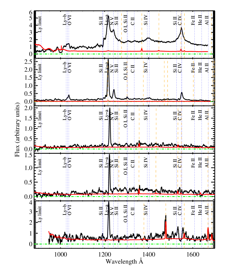
Figure 2: Figures 2 to 4 present individual spectra of the 13 Lyman break galaxies and 2 QSOs that reside within $\Delta z=0.0125$ of the 11 DLAs. In addition, we include the spectra of two LBGs found within $\Delta z=0.015$ of the $z=2.936$ DLA in the PSS0808+5215 field. Error arrays are overlaid (in red) and expected interstellar and stellar absorption lines are indicated using vertical dotted (blue) lines. Bright night sky emission lines, that can be difficult to subtract completely in fainter spectra, are marked with vertical dashed (orange) lines. These spectra range from the lowest to highest signal-to-noise ratio of the complete sample. They are smoothed by 15 pixels for clarity over the wavelength range shown and to help highlight the break(s) in the continua, however the sharpness of the individual emission and absorption lines is affected. Top to bottom: Objects 0336-0782 (QSO found near the DLA in the PKS0336–017 field), 0957-0859 (QSO found near the DLA in the PSS1057+4555 field), 1013-0210, 1013-0661, & 0056-0993.

Figures 2 through 4 present the individual spectra of the 15 systems (13 LBGs and 2 QSOs) within $\Delta z=0.0125$ of the 11 DLAs in this survey. In addition, we have included the spectra of two LBGs found within $\Delta z=0.015$ of the $z=2.936$ DLA in the PSS0808+5215 field (see §6.3.2). The low signal-to-noise spectra have been smoothed by 15 pixels. This large smoothing allows the coarse features of the continua to be seen more readily on the wavelength scales presented here, but diminishes the appearance of individual absorption features. These range from the highest to the lowest signal-to-noise ratio spectra in the complete sample. As presented in Paper I, these spectra are best referenced to, and studied as, composite spectra of galaxies displaying similar spectral profiles.

In nearly every spectra, a decrement in the continuum is visible shortward of 1216Å caused by absorption from optically thick intervening systems at lower redshift (the Lyman $\alpha$ forest). LBGs are faint sky-dominated objects and bright night sky emission lines can be difficult to subtract cleanly from the spectra. Therefore, the positions of the sky emission lines are marked to prevent the misidentification of residual sky flux as real LBG features. No order blocking filter was used in these observations resulting in an underestimation of the flux longward of $\sim 6300$Å in the observation frame or longward of $\sim 1500$Å in the rest-frame.

Overall, the spectra of the systems near DLAs appear to be those of typical LBGs and we find a similar ratio of emission-identified LBGs to absorption-identified LBGs as in the complete sample. Excluding QSOs, the 15 LBGs presented here exhibit a magnitude range of $23.1<$ R $<25.4$. The set of 205 LBGs with no apparent AGN activity has a magnitude range of $22.1<$ R $<25.5$, where R $=25.5$ is the practical spectroscopic magnitude limit of Keck using the LRIS instrument. The R magnitude distribution of these objects against the full set of LBGs are shown in Figure 5. A two-sided Kolmogorov-Smirnov test resulted in a value of 0.6 and a high probability that the cumulative distribution functions of both datasets are significantly similar.

4 Faint AGN

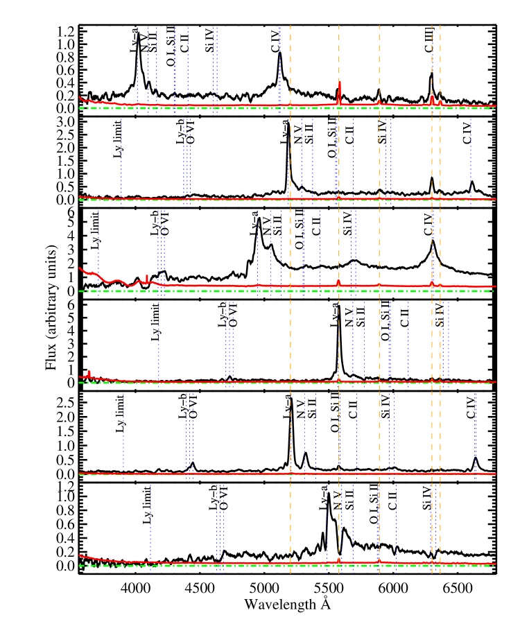
Figure 6: Spectra of the six $20.0<$ R $<25.5$ QSOs discovered in this survey with the error arrays are overlaid (in red). Some identified emission and absorption lines are marked with vertical dotted (blue) lines and labeled. Bright night sky emission lines are marked with vertical dashed (orange) lines. Night sky lines can be difficult to subtract completely in the fainter spectra. Top to bottom: 0056-1085, 0336-0645, 0336-0782, 0808-0876, 0957-0859, & 1057-3225.

Figure 6 presents the smoothed spectra of six Lyman break objects displaying AGN activity discovered in the 465 arcmin² of this survey. These six $20.1<$ R $<24.4$ objects are separate and distinct from the nine QSOs targeted in this survey and result in a faint AGN number density of $\sim 46\deg^{-2}$. Three objects are broad-line AGN with FWHM $>2000$ km s^-1 and display several broad emission features that are typical of QSOs, and the remaining three display emission lines with FWHM $<2000$ km s^-1 including Lyman $\alpha$ and at least one other high ionization species indicative of a hard spectrum. The spectrum of object 0808-0876 did not extend to Civ $\lambda\lambda 1548,1551$, but detailed inspection does show Ovi $\lambda\lambda 1032,1038$, Nv $\lambda 1240$, and possible Siv $\lambda\lambda 1394,1402$ emission. As a result, this object can not be ruled out as a Lyman break galaxy in the conventional sense of the term.

Interestingly, two of the six QSOs were discovered within $\Delta r_{z}=0.0125$ ($<10h^{-1}$Mpc) of two DLAs. Object 0957-0859, an R $=23.3$ narrow-line QSO at $z=3.283$, lies near the $z=3.279$ DLA in the PSS0957+3308 field at an angular separation of 241 arcsec. Object 0336-0782 at $z=3.074$ is a brighter R $=20.1$ broad-line QSO and lies at an angular separation of 167 arcsec from the $z=3.062$ DLA in the PKS0336–017 field. Since the appearance of two QSOs at small separations from the two DLAs seemed unlikely, we tested this in the following manner. We assumed the detection of one QSO per survey DLA field (we found six QSOs in nine fields) and ran a Monte Carlo simulation of 10,000 realizations corrected by the photometric selection function. From this, we estimate a 3.8% and 2.8% chance that a QSO would reside randomly within $\Delta r_{z}=0.0125$ of the $z=3.062$ and $z=3.279$ DLA, respectively. More importantly, we estimate 1 chance in 940 that a QSO would reside within $\Delta r_{z}=0.0125$ of both DLAs. This is significant to $\sim 4\sigma$ and may have important implications on the distribution of QSOs with DLAs. The close proximity of the QSOs with the DLAs may provide insight into the duty cycle of QSOs and the overall size and survival of high column-density neutral gas reservoirs in environments with sources of significant ionizing flux. More research into this relationship is necessary and is one of the goals of our ongoing One-Degree Deep survey (Cooke et al., 2006b).

In the following sections, we focus on the distribution of the LBG population as a whole. Throughout, we search for evidence of an overdensity of LBGs near DLAs over random and compare this to the overdensity of LBGs near other LBGs. We describe the approach adopted to estimate the three-dimensional LBG auto-correlation and DLA-LBG cross-correlation functions and present several techniques to measure and test these functions from the dataset.

5 Correlation Functions: Methodology

For a random distribution of LBGs, the joint probability of finding an LBG occupying volume element $dV_{1}$ and another LBG occupying volume element $dV_{2}$ at a separation $r$ is (Peebles, 1980)

$$dP(r)=\bar{n}_{LBG}^{2}~{}dV_{1}dV_{2}$$ (11)

where $\bar{n}_{LBG}$ is the mean density of LBGs averaged over the realization. In general, for any given distribution of LBGs, this expression becomes

$$dP(r)=\bar{n}_{LBG}^{2}~{}[1+\xi_{LBG}(r)]dV_{1}dV_{2}$$ (12)

where $\xi_{LBG}(r)$ is the LBG auto-correlation function. In this context, $\xi_{LBG}(r)$ quantifies the excess probability over random.

Similarly, for two populations (here DLAs and LBGs), the joint probability of finding an object from the first population at a distance $r$ from an object of the second population is

$$dP(r)=\bar{n}_{DLA}\bar{n}_{LBG}~{}[1+\xi_{DLA-LBG}(r)]~{}dV_{DLA}dV_{LBG}$$ (13)

where $\bar{n}_{DLA}$ is the mean density of DLAs and $\xi_{DLA-LBG}(r)$ is the cross-correlation function also quantifying the excess probability over random. From this, the conditional probability of finding an LBG at a distance $r$ from a known DLA is

$$dP(r)=\bar{n}_{LBG}~{}[1+\xi_{DLA-LBG}(r)]~{}dV_{LBG}.$$ (14)

Based on studies of nearby galaxies it has been commonly assumed that $\xi(r)$ follows a power law of the form

$$\xi(r)=\left(\frac{r}{r_{0}}\right)^{-\gamma}.$$ (15)

This has been a reasonable assumption given that the power spectrum is well fit by a power law and that $\xi(r)$ is essentially the Fourier transform of the power spectrum. In this form, the parameters $r_{0}$ and $\gamma$ are all that are needed to describe the correlation function. In practice, $\xi(r)$ is estimated by comparing the galaxy separations found in the data to the galaxy separations in mock catalogs of randomly distributed galaxies. These random galaxy catalogs mimic the angular and spatial configuration of the data [e.g. Davis & Peebles (1983); Hawkins et al. (2003); Adelberger et al. (2003)]. By carefully restricting the random galaxy catalogs to the exact constraints of the real data, complications caused by edge effects, bright objects, and the physical constraints of the instruments are removed or well constrained.

5.1 Spatial correlation estimator

There have been several methods proposed and used to estimate $\xi(r)$ from galaxy catalogs. We adopt the method of Landy & Szalay (1993) which is well-suited for small galaxy samples and has the least bias present in commonly used estimators (Kerscher et al., 2000). This technique involves comparing the number of galaxy pairs in the data having separations within a given spatial interval $r\pm\delta r$ to the number of galaxy pairs in the random galaxy catalogs having separations within the same spatial interval. To reduce shot noise, the random galaxy catalogs are made many times ($\sim 100$ times) larger than the data sample and normalized to the data. The number of pairs is counted in each spatial bin determined in logarithmic or linear space. From the normalized bin counts, the LBG auto-correlation function $\xi_{LBG-LBG}~{}(r)$ is estimated as

$$\xi_{LBG-LBG}~{}(r)=\frac{D_{LBG}D_{LBG}-2\cdot D_{LBG}R_{LBG}+R_{LBG}R_{LBG}}{R_{LBG}R_{LBG}}$$ (16)

and the DLA-LBG cross-correlation function $\xi_{DLA-LBG}(r)$ is estimated as

$$\xi_{DLA-LBG}~{}(r)=\frac{D_{DLA}D_{LBG}-D_{DLA}R_{LBG}-R_{DLA}D_{LBG}+R_{DLA}R_{LBG}}{R_{DLA}R_{LBG}}$$ (17)

where the separations between galaxies in the data constitute the $DD$ catalogs, separations between random galaxies make up the $RR$ catalogs, and separations between data and random galaxies make up the $DR$ and $RD$ cross-reference catalogs. Equations 16 & 17 are identically used to estimate the projected angular correlation functions $\omega_{p}$ in § 6.1.

6 Correlation Functions: Results by Technique

We present several approaches to measure and test for an overdensity of LBGs near LBGs and LBGs near DLAs over random. We first describe the correlation functions as determined by a conventional binning technique. We find a dependence of the correlation function on bin parameters and circumvent this shortcoming, which can be pronounced for small datasets, by performing a maximum likelihood analysis and comparing the results. The maximum likelihood method makes the most of the dataset and is a direct and essentially bin-independent way to determine the clustering behavior. Lastly, we test the effects that the physical constraints of the slitmasks and the presence of an individual overdense field have on the correlation function. The redshift separations in all analyses were determined in a consistent manner.

6.1 Conventional binning

We followed the modification to conventional radial bins suggested by A03 in an effort to diminish the effects that the LBG redshift uncertainties caused by galactic-scale winds have on the clustering amplitude. In doing so, we also provide a means for direct comparison by methodology of our measure of the LBG auto-correlation and the DLA-LBG cross-correlation functions to the LBG auto-correlation function of A03. In this treatment, the number of pairs is counted that reside in concentric “cylindrical” bins with dimensions $r_{\theta}\pm\delta r_{\theta}$ and $r_{z}\pm\delta r_{z}$. Limits are placed on $r_{z}$ such that it is the greater of $7r_{\theta}$ and 1000 km sec${}^{-1}(1+z)/H(z)$ and chosen to be several times larger than the redshift uncertainties. Here we interpreted $(1+z)$ as $(1+\bar{z})$ where $\bar{z}$ is the average redshift of the two objects. The length in redshift of each bin is fixed ($\sim 9h^{-1}$Mpc at $z\sim 3$) for small $r_{\theta}$ and grows as $7r_{\theta}$ when $r_{\theta}$ becomes large. The lower limit is placed to avoid missing correlated pairs and the upper limit reaches down the correlation function to include $>80\%$ of the correlated pairs for $\gamma\gtrsim 1.6$.

We measured out to the maximum angular separation of $\theta=300^{\prime\prime}$ and used logarithmic $r_{\theta}\pm dr_{\theta}$ bins to remain consistent with the parameters chosen by A03. Recalling that the fields in this survey are $\sim 6^{\prime}\times 7.5^{\prime}$, the number of pairs with separations at larger radii diminishes rapidly. Assuming the canonical power law form of the correlation function (equation 15), the expected excess number of pairs using this approach is

$$\omega_{p}(r_{\theta},<r_{z})\equiv\frac{\langle n\rangle}{\bar{n}}-1=\frac{r_{0}^{\gamma}r_{\theta}^{1-\gamma}}{2r_{z}}B\left(\frac{1}{2},\frac{\gamma-1}{2}\right)I_{x}\left(\frac{1}{2},\frac{\gamma-1}{2}\right)$$ (18)

where $\langle n\rangle$ is the expected number of objects, $\bar{n}$ is the number of objects in a random sightline, $B$ and $I_{x}$ are the beta and incomplete beta functions with $x\equiv r_{z}^{2}(r_{z}^{2}+r_{\theta}^{2})^{-1}$ (Press et al. 1992, §6.4). The best fit values of $r_{0}$ and $\gamma$ of the correlation function result from fitting equation 18 to the observed number of pairs measured by the above binning scheme. The fundamental errors in $\omega_{p}$ are dependent on our choice of estimator. Using the estimators in equations 16 & 17, the errors $\delta\omega_{p}(\theta)$ are described by (Roche et al., 1999; Foucaud et al., 2003)

$$\delta\omega_{p}(\theta)=\sqrt{\frac{1+\omega_{p}(\theta)}{DD}}$$ (19)

where $DD$ represents either the $D_{LBG}D_{LBG}$ or $D_{DLA}D_{LBG}$ pair catalogs.

The uncertainties of the functional fits were estimated by running a Monte Carlo simulation of the measured correlation function. As described in Appendix C, A03, this approach is to create a large number (we performed 1000) of realizations of $\omega_{p}$ by adding a Gaussian deviate to the fundamental error and minimizing the $\chi^{2}$ fit. The range of 68% of the best fit parameter values is what we report as the best fit value $1\sigma$ uncertainty when using this method. These uncertainties may be underestimated by a factor of $1-2$, as argued in Adelberger et al. (2005) and Adelberger (2005).

6.1.1 LBG auto-correlation

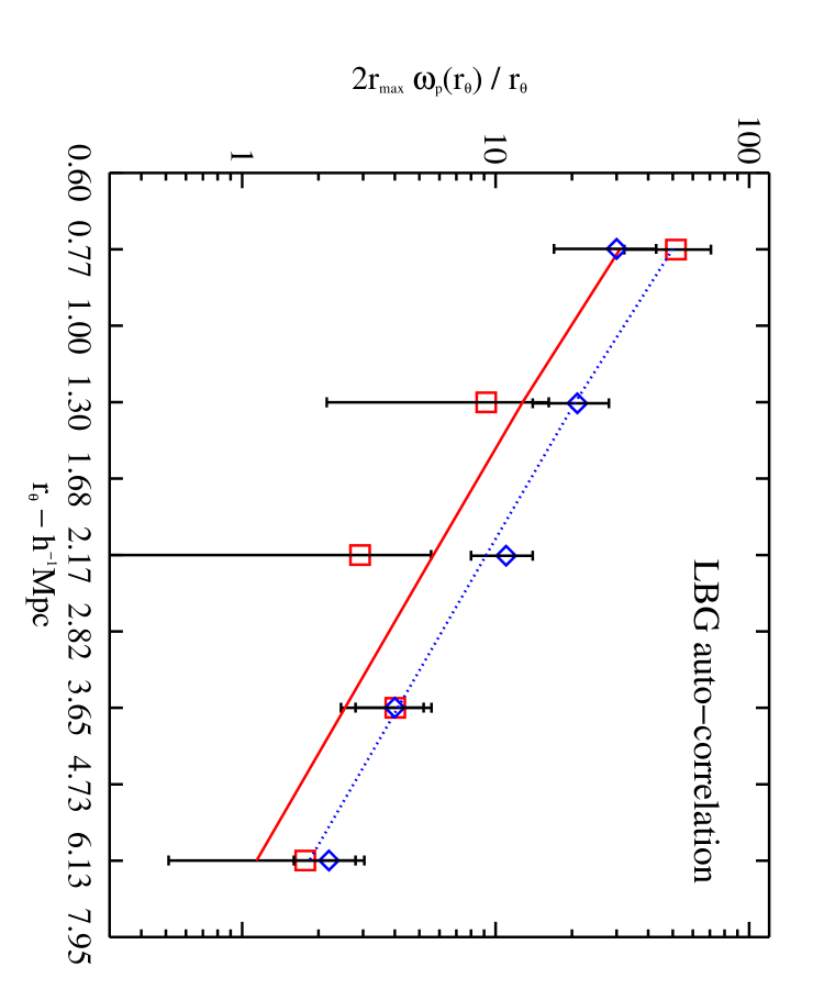
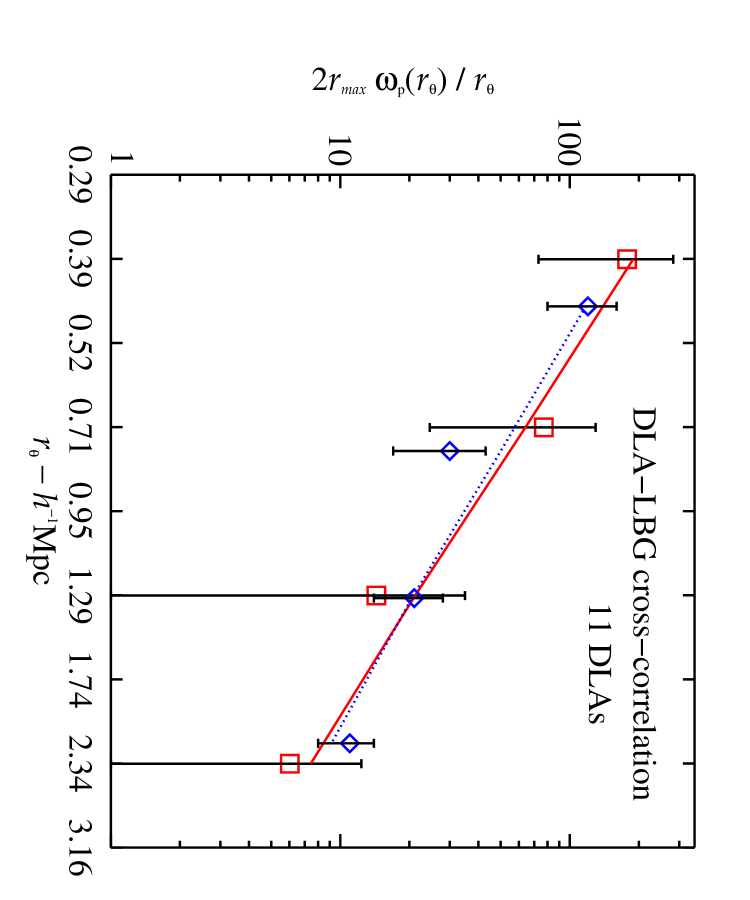
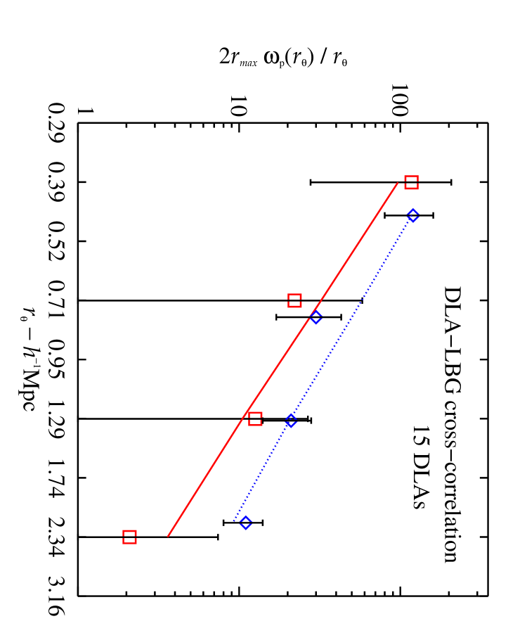
Figure 7: Plot of the LBG auto-correlation and DLA-LBG cross-correlation functions using the binning technique described in the text. The correlation functions are shown as (red) squares and best fit as the solid (red) lines. We measure the best fit values and $1\sigma$ errors of $r_{0}=2.65\pm 0.48,\gamma=1.55\pm 0.40$ for the LBG auto-correlation (upper panel), $r_{0}=3.32\pm 1.25,\gamma=1.74\pm 0.36$ for the DLA-LBG cross-correlation of the 11 DLAs in this survey (center panel), and $r_{0}=2.70\pm 1.16,\gamma=1.73\pm 0.39$ for the DLA-LBG cross-correlation of the combined set of 15 DLAs (lower panel) that includes four DLAs from the survey of Steidel et al. (2003). The errors shown are those determined by equation 19. Overlaid in (blue) diamonds are the data for the LBG auto-correlation from Adelberger et al. (2003) and best fit to that data, marked by the dotted (blue) lines, for comparison.

A03 reported the values and $1\sigma$ uncertainties of $r_{0}=3.96\pm 0.29$ and $\gamma=1.55\pm 0.15$ for the LBG auto-correlation at $z\sim 3$. As stated above, we fit our data in an identical manner as A03 including the Monte Carlo error analysis. The best fit values and $1\sigma$ uncertainties for our dataset are $r_{0}=2.65\pm 0.48$ and $\gamma=1.55\pm 0.40$ and is shown in Figure 7, with the published results of A03 overlaid for comparison. The bin errors shown in the figure (and all subsequent figures by this method) are the error estimates on $\omega_{p}$ using equation 19. We find a possibly weaker clustering amplitude for $z\sim 3$ LBGs in our sample as compared to A03, yet consider the possible error underestimation on the functional fit to the data as mentioned above. In addition, subtleties involved in random catalog generation, sample variance and sample size, estimation of the $U_{n}G\cal R$I versus $u^{\prime}$BVRI photometric selection function profiles, LBG redshift assignments, and our inability to accurately measure the correlation function at separations smaller than $\sim 0.5h^{-1}$Mpc may contribute as well. In the remaining plots, all comparisons of the best fit values for the LBG auto-correlation and the DLA-LBG cross-correlation must consider these possible differences.

6.1.2 DLA-LBG cross-correlation

We performed the above binning technique on the cross-catalogs of DLA and LBG separations to determine the first spectroscopic measure of the DLA-LBG cross-correlation function. The best fit to the cross-correlation data resulted in values and $1\sigma$ uncertainties of $r_{0}=3.32\pm 1.25$ and $\gamma=1.74\pm 0.36$ (Cooke et al., 2006a) and is shown in Figure 7. Upon inspection, it is immediately apparent that the DLA-LBG cross-correlation function has a similar slope and correlation length as the LBG auto-correlation function. The angular range of the plot ($\sim 0.4-3h^{-1}$Mpc) reflects the limits on the correlation measurement caused by placing the DLAs in the center of our images. Although the uncertainty in either cross-correlation parameter is large, the measured central values indicate an overdensity of LBGs near DLAs to $1-2\sigma$.

6.1.3 Inclusion of previous work

The data from the four DLAs in the survey of Steidel et al. (2003), hereafter S03, and the 11 DLAs from this work constitute the largest available spectroscopic sample of DLAs and LBGs to measure the spatial DLA-LBG cross-correlation function. The similarity in techniques and instruments used in both surveys allowed a direct combination of the data once the few differences were addressed and corrected to the best of our abilities. We used the available online dataset of S03 and note that our knowledge of some aspects of those observations were limited. In lieu of Lyman $\alpha$ equivalent width information for each LBG in their sample, we were restricted to using equations 8 and 10 to determine the systemic redshifts of 880 LBGs in 17 fields [and later a sub-sample of 700 in 15 fields from Adelberger (2004)]. The area of each S03 field was estimated by the extent of the angular positions of their spectroscopic data (this assumes a position angle identical to, or having a right angle to, PA=0 for each slitmask). Random catalogs were generated in the same manner as described above using these field sizes and the observed density of their sample.

Once we were satisfied with our duplication of the LBG auto-correlation of A03, we measured the best fit values and $1\sigma$ uncertainties of $r_{0}=2.20\pm 0.96$, $\gamma=1.77\pm 0.40$ for the DLA-LBG cross-correlation for the full set of 15 DLAs. The results are presented in Figure 7. It can be seen that evidence for an overdensity of LBGs near DLAs survives and, acknowledging the above caveats and our efforts to correct the differences between the two surveys, the 15 DLAs may provide a better sample to determine the cross-correlation parameters of DLAs at $z\sim 3$.

6.2 Maximum likelihood

Arbitrary binning of the data into coarse bins introduces uncertainties because the value of $\xi(r)$ can depend on the bin size, interval, and bin center. Dependence on bin size is illustrated in Figure 8. In that plot, we varied the bin size from logarithmic intervals of $0.225$ to $1.125$ over a fixed $r_{\theta}\sim 0.04-8h^{-1}$Mpc and found that $r_{0}$ varied from $\sim 2.0-3.1h^{-1}$ Mpc and $\gamma$ varied from $\sim 1.35-1.48$ in our analysis of the S03 sample. To remedy this problem, we estimated the value of $r_{0}$ and $\gamma$ in the most direct way possible. We maximized the likelihood that a power law of the form $\xi(r)=(r/r_{0})^{-\gamma}$ would produce the observed pair separations (Croft et al., 1997; Mullis et al., 2004).

Poisson probabilities are valid in the limit where the number of bins is large and the probability per bin is small. Constructing bin separations on such a fine level as to include either one or zero LBGs per bin allows us to form the likelihood function. The probabilities associated with the bins are assumed independent of each other in the sparse sampling limit. The probability $P$ of finding $\nu_{i}$ observed pairs where $\mu_{i}$ pairs are expected is the Poisson probability

$$P_{\mu_{i}}(\nu_{i})=\frac{e^{-\mu_{i}}\mu_{i}^{\nu_{i}}}{\nu_{i}!}.$$ (20)

The likelihood function $\cal L$ is the product of the probability of having exactly one pair in every interval where one pair exists in the data and exactly zero in all others and is defined in terms of the joint probabilities

$${\cal L}=\prod_{i}^{N}\frac{e^{-\mu_{i}}\mu_{i}^{\nu_{i}}}{\nu_{i}!}\prod_{j\neq i}^{N}\frac{e^{-\mu_{j}}\mu_{j}^{\nu_{j}}}{\nu_{j}!}$$ (21)

where $\mu_{i}$ is the expected number of pairs in the interval $dr$, $\nu_{i}$ is the observed number of pairs for that same interval, and the index $j$ runs over the elements where there are no pairs. This can also be expressed as

$$\ln{\cal L}=\sum_{i}^{N}(-\mu_{i}+\nu_{i}\ln\mu_{i}-\ln\nu_{i}!)+\sum_{j\neq i}^{N}(-\mu_{j}+\nu_{j}\ln\mu_{j}-\ln\nu_{j}!).$$ (22)

The expected number of objects $\mu_{i}$ for a given radial separation is obtained by solving equations 16 & 17 for $D_{LBG}D_{LBG}$ and $D_{DLA}D_{LBG}$, respectively. As stated above, we used the assumption that $\xi(r)=(\frac{r}{r_{0}})^{-\gamma}$ (equation 15) and varied the values of both $r_{0}$ and $\gamma$ to determine the values of maximum likelihood. The maximum likelihood was determined by minimizing the conventional expression

$$S=-2\ln{\cal L}$$ (23)

and using $\Delta S=S(r_{best},\gamma_{best})-S(r_{0},\gamma)$ to determine $\chi^{2}$ confidence levels, observing that the values of $S$ had $\chi^{2}$ distributions.

The maximum likelihood technique is a powerful tool in measuring the likelihood of a given functional fit to the data but has at least one shortcoming in the form presented here. As mentioned above, the Poisson approximation is valid in the regime large interval number (very small separation radius) and low probability. But, even large random catalogs will occasionally find zero pairs in the very small intervals where this approximation is most accurate. In these cases, the likelihood may be less accurate or undefined. Therefore, we imposed the following two conditions (Mullis, 2005): (1) the number of separations in the data-random cross-catalogs $DR$ (and $RD$) must be greater than zero for each bin which indirectly imposes the same condition on the random-random catalogs $RR$ since they are larger, and (2) imposing the constraint that $[\xi(r)-1]>2DR/RR$ (or $[\xi(r)-1]>(DR+RD)/RR$ for the cross-correlation). For the few values of $r$ where this criteria was not met the expected value of $DD$ was interpolated across the finely spaced intervals. Interpolating the few instances where this occurred had little impact on the final result because there were far fewer of these intervals when compared to the total used for analysis.

6.2.1 LBG auto-correlation

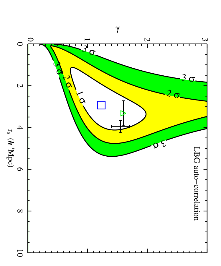
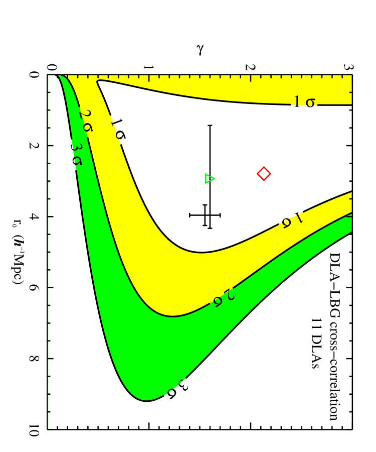
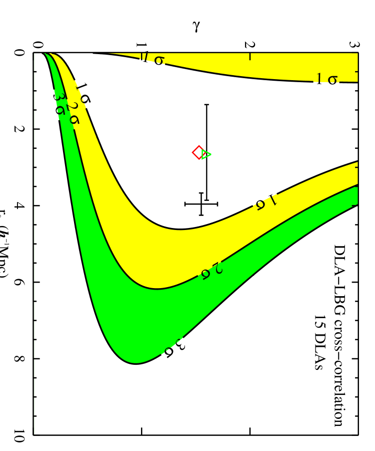
Figure 9: Correlation function probability contours for two free parameters as measured by the maximum likelihood method. Top panel: The (blue) square at $r_{0}=2.91$, $\gamma=1.21$ marks the maximum likelihood values for the LBG auto-correlation for our survey. Middle panel: The (red) diamond marks the maximum likelihood values of $r_{0}=2.81$ and $\gamma=2.11$ for the DLA-LBG cross-correlation. Bottom panel: The (red) diamond marks the maximum likelihood values $r_{0}=2.66$, $\gamma=1.59$ for the DLA-LBG cross-correlation for the combined sample of 11 DLAS from this survey and the four DLAs from the survey of Steidel et al. (2003). The (green) triangles on each plot and $1\sigma$ error bars are the best fit values (one free parameter) of $r_{0}$ for a fixed value of $\gamma=1.6$. The error crosses indicate the values and $1\sigma$ errors for the LBG auto-correlation as determined by Adelberger et al. (2003). The 1, 2, and 3 $\sigma$ confidence regions are labeled.

The maximum likelihood values for the LBG auto-correlation and $1\sigma$ confidence levels were found to be $r_{0}=2.91^{+1.0}_{-1.0}$ and $\gamma=1.21`^{+0.6}_{-0.3}$. The probability contours are shown in the top panel Figure 9 where, in addition, we overlay both the maximum likelihood value and $1\sigma$ confidence level of $r_{0}$ for a fixed $\gamma=1.6$ and the best fit values and $1\sigma$ errors of the LBG auto-correlation function of A03 for comparison. The values of $r_{0}$ and $\gamma$ determined by this method are consistent to within their errors with those found using conventional binning, Moreover, the maximum likelihood technique yields the same results regardless of the number intervals tested.

6.2.2 DLA-LBG cross-correlation

Since the maximum likelihood method is well-suited for small samples, we readily applied it toward the DLA-LBG cross-correlation measurement. The analysis found maximum likelihood values and $1\sigma$ confidence levels of $r_{0}=2.81^{+1.4}_{-2.0}$ and $\gamma=2.11^{+1.3}_{-1.4}$ for the set of 11 DLAs and $r_{0}=2.66^{+1.9}_{-2.1}$ and $\gamma=1.59^{+1.6}_{-0.9}$ for the full set of 15 DLAs, with the probability contours shown in Figure 9 (center and bottom panel, respectively). We found that $65-90$% of the maximum likelihood values indicate a non-zero $r_{0}$ depending on the value of $\gamma$. Although the uncertainties are large, the best fit values using the maximum likelihood technique also suggest an overdensity of LBGs near DLAs with $1-2\sigma$ confidence similar to the results using conventional binning.

6.3 Tests

This survey uses the distribution of LBGs determined from multi-object spectroscopic data to measure the correlation functions. Here we test the contributions to the correlation functions by the physical constraints of the multi-object slitmasks and test the strength of the clustering signal in the absence of the DLA having the largest overdensity of LBGs.

6.3.1 Physical constraints of the observations

A false enhancement of the clustering signal can occur when the finite number of multi-object slitmasks do not cover the full area of the imaged fields. This effect can be problematic in every survey and is nearly removed here by the fact that seven out of the nine fields were imaged with the relatively small field-of-view LRIS camera and have spectroscopic coverage over their entire area. The remaining two fields, imaged by the larger field-of-view COSMIC, have $\sim 70\%$ areal spectroscopic coverage. However, any augmentation to the correlation functions from these two fields was virtually eliminated by confining our random catalogs to the precise areas sampled by the slitmasks and by the fact that these two fields have few spectra and make a small contribution to the final results.

Perhaps a more prominent effect is the dilution to the clustering signal from the fact that only a finite number of objects are allowed on each slitmask. All but one of the LBG candidates that lie in conflict in the dispersion direction are compromised. Similarly, LBGs that cluster tightly in angular space require many slitmasks for proper spectroscopic coverage which is not usually feasible. In order to minimize this, we observed two to three overlapping slitmasks in most fields. Even so, there remain a few tightly clustered LBG candidates as well as LBG candidates that were in conflict in the dispersion direction that have no spectral coverage to date. To measure the extent in which this physical constraint affects the clustering signal, we compared the results of the correlation functions using random catalogs having galaxies with the exact angular positions of the data to those using random catalogs having galaxies with random angular positions.

The correlation measurements presented in §6.1 & §6.2 used random galaxy catalogs having the exact angular positions of the data. We re-measured the correlation functions using these techniques but allowed the galaxies in the random catalogs to have random angular positions. Doing so, we found the best fit parameters and $1\sigma$ uncertainties for the LBG auto-correlation to be $r_{0}=2.31\pm 0.55$, $\gamma=1.47\pm 0.40$ for the conventional binning method and $r_{0}=2.08^{+1.0}_{-1.1}$, $\gamma=1.49^{+1.1}_{-0.5}$ for the maximum likelihood method. Duplicating this for the DLA-LBG cross-correlation of the 11 DLAs in our survey [and the combined set of 15 DLAs], we found the best fit parameters and $1\sigma$ uncertainties to be $r_{0}=3.21\pm 0.95$, $\gamma=2.03\pm 0.22$ [$r_{0}=2.52\pm 0.92$, $\gamma=1.71\pm 0.46$] using conventional binning and $r_{0}=3.20^{+2.2}_{-2.9}$, $\gamma=1.62^{+1.4}_{-1.0}$ [$r_{0}=2.44^{+1.3}_{-1.9}$, $\gamma=2.41^{-1.6}_{-1.7}$] using the maximum likelihood technique. There was no apparent trend in either parameter which suggests that the physical constraints of the slitmasks had a weak effect on our survey as a whole. This was suspected since, in most cases, we obtained overlapping spectroscopic coverage. Although the central values of the parameters are increased in some cases and decreased in others, they are within error in all cases.

6.3.2 The PSS0808+5215 field

Field-by-field analysis revealed a relative spike of five LBGs with $\Delta z<0.015$ ($<10h^{-1}$Mpc) to the $z=2.936$ DLA in the PSS0808+5215 field. A redshift histogram of the $2.6<z<3.4$ LBGs in the PSS0808+5215 field is shown in Figure 10. To estimate the probability of this overdensity occurring by chance, we ran 10,000 random simulations of the distribution of the $2.6<z<3.4$ LBGs detected in the field corrected by the photometric selection function. We found five LBGs within $\Delta z=0.015$ of the $z=2.936$ DLA $0.16\%$ of the time. Therefore, we conclude that this is most likely a real overdensity. To illustrate the extent of the overdensity, Table 2 lists the number of LBGs in cells centered on the $z=2.936$ DLA with varying radius in redshift. We find the next nearest LBG at $\Delta z=0.043$, or $29.9h^{-1}$ Mpc.

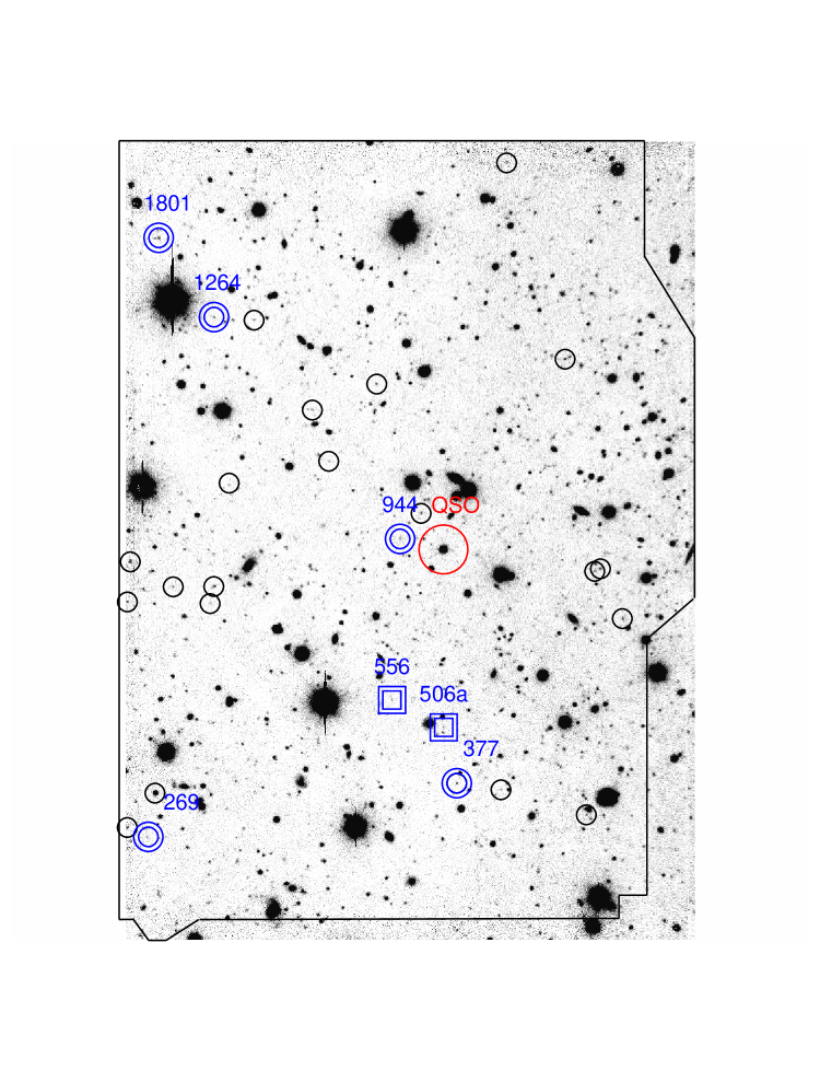
Figure 11: R-band image of LBGs identified in the PSS0808+5215 field. The central $z=4.45$ QSO displays DLAs at $z=2.936$ and $z=3.114$. The QSO is indicated by the large (red) circle. The five LBGs associated with the $z=2.936$ DLA are shown using two concentric (blue) circles and the two LBGs associated with the $z=3.114$ DLA are shown using two concentric (blue) squares. All other spectroscopically confirmed LBGs are shown as small (black) circles. The LRIS field size is $\sim 5.5^{\prime}\times 7^{\prime}$ which corresponds to comoving $\sim 7\times 10h^{-1}$Mpc. The region bounded in black is the area covered by the three slitmasks used on this field.

Inspection of the angular distribution of the LBGs in the two-dimensional image indicates we may not be seeing the full extent of the overdensity because of the relatively small field of view of the LRIS camera. In fact, this is true for all fields imaged with the LRIS camera. Figure 11 presents an R-band image of the PSS0808+5215 field. The QSO and spectroscopically confirmed $z>2$ LBGs are marked in the image with the LBGs near the $z=2.936$ and $z=3.114$ DLA are indicated separately. The DLA at $z=2.936$ appears to reside toward the apparent edge of the overdensity. This is an excellent argument for the acquisition of wide-field images in future surveys and is one of the main objectives of our One-Degree Deep survey. Clustering analysis on scales much larger than the correlation length is necessary for the proper correlation analysis and study of large-scale behavior of LBGs and DLAs.

To test how this overdensity affected the overall DLA-LBG clustering amplitude, we computed the strength of the cross-correlation in the absence of the $z=2.936$ DLA. We found best fit values and $1\sigma$ errors of $r_{0}=2.98\pm 1.34$ and $\gamma=1.32\pm 0.34$ using the conventional binning technique and $r_{0}=2.72^{+1.8}_{-2.1}$, $\gamma=1.48^{+1.5}_{-1.1}$ using the maximum likelihood method. The survival of the clustering signal after the omission of the $z=2.936$ DLA in the PSS0808+5215 field is further evidence for an overdensity of LBGs near DLAs on average. In fact, from every measurement and test in this work, a non-zero clustering signal has been detected.

7 Galaxy bias and mass

The primary objective of this survey was to measure the DLA-LBG cross-correlation function to estimate the DLA galaxy bias in the context of CDM cosmology and use this information to infer the average halo mass of DLAs. This provides a first step in establishing the fundamental properties of the population of proto-galaxies that DLAs represent. We were successful in making an independent measurement of the LBG auto-correlation function at $z\sim 3$ and used this as an important calibrator to measure the DLA-LBG cross-correlation function. Although the uncertainties in this work make a direct measure of the DLA bias difficult, it can be estimated in the following way. The relationship between the LBG auto-correlation function $\xi_{LBG}$ and dark matter correlation function $\xi_{DM}$ on scales where the linear bias is a good model is

$$\xi_{LBG}(r)=b_{LBG}^{2}~{}\xi_{DM}(r),$$ (24)

where $b_{LBG}$ is the LBG galaxy bias. Similarly, for the DLA-LBG cross-correlation function the relationship is

$$\xi_{DLA-LBG}(r)=b_{DLA}b_{LBG}~{}\xi_{DM}(r)$$ (25)

(Gawiser et al., 2001) where $b_{DLA}$ is the DLA galaxy bias. Therefore, the ratio of the two relationships becomes

$$\frac{\xi_{DLA-LBG}(r)}{\xi_{LBG}(r)}=\frac{b_{DLA}}{b_{LBG}}.$$ (26)

Assuming, as we have throughout this paper, that $\xi(r)$ is well fit by a power law of the form $\xi(r)=(r/r_{0})^{-\gamma}$, and assuming identical values of $\gamma$ for both the auto-correlation and cross-correlation functions, this ratio becomes

$$\left(\frac{r_{0LBG}}{r_{0DLA-LBG}}\right)^{-\gamma}=\frac{b_{DLA}}{b_{LBG}}$$ (27)

and illustrates that the ratio of the correlation lengths is a direct indicator of the ratio of the biases. These assumptions are reasonable, especially when considering that both $r_{0}$ and $\gamma$ were freely varied when fitting the LBG auto-correlation and DLA-LBG cross-correlation functions using each technique and produced consistent values within their uncertainties (Tables 3 & 4). Moreover, we measured the best fit values of $r_{0}$ for each correlation function at various values of fixed $\gamma$ and found all resulting correlation lengths to be in agreement within error as well. Table 5 displays the best fit values for a fixed value of $\gamma=1.6$.

It is true that the DLA-LBG cross-correlation function measurement from each method individually can only confirm a non-zero DLA galaxy bias with $\sim 1-2\sigma$ confidence. But the implications from the combined set of measurements and tests of those measurements are what drive our overall claim that DLAs and LBGs likely have a similar spatial distributions and galaxy bias. The results indicate not only an overdensity of LBGs near DLAs over random, but correlation functions of similar form and strength. We find that the average correlation lengths and uncertainties for fixed and varied values of $\gamma$ for the LBGs in this work correspond to an average $z\sim 3$ LBG galaxy bias between $2<b_{LBG}<3$ and $1.5<b_{LBG}<3$ respectively. Similarly, the average $z\sim 3$ DLA galaxy bias ranges between $1.3<b_{DLA}<4$ and $1.5<b_{DLA}<4$ for the 11 DLAs in this survey and $1.3<b_{DLA}<3$ and $0.8<b_{DLA}<3$ for the combined set of 15 DLAs. The average halo mass of a galaxy population can be inferred from the galaxy bias using halo mass function approximations, e.g., Mo et al. (1998); Sheth, et al. (2001). The above galaxy bias values correspond to LBG mass ranges of approximately $10^{10.8}<\langle M_{LBG}\rangle<10^{11.6}~{}M_{\odot}$ and $10^{9.7}<\langle M_{LBG}\rangle<10^{11.6}~{}M_{\odot}$, respectively. The average measurements for the 11 DLAs in this survey lead to approximate mass ranges of $10^{9}<\langle M_{LBG}\rangle<10^{11.9}~{}M_{\odot}$ and $10^{9.7}<\langle M_{LBG}\rangle<10^{12}~{}M_{\odot}$ and approximate mass ranges for the combined set of 15 DLAs of $10^{9}<\langle M_{LBG}\rangle<10^{11.6}~{}M_{\odot}$ and $10^{7.3}<\langle M_{LBG}\rangle<10^{11.7}~{}M_{\odot}$, for fixed and varied values of $\gamma$ respectively in each case. Both the galaxy bias and mass calculations were determined by the method outlined in Quadri et al. (2006).

The $z\sim 3$ LBG correlation length computed by A03 is $3.96\pm 0.29$ for the $\cal{R}$ $<25.5$ spectroscopic sample results in an LBG galaxy bias of $b_{LBG}\sim 4$ and corresponds to an average halo mass of $\langle M_{LBG}\rangle\sim 10^{11.9}~{}M_{\odot}$. In addition, it has been shown that the LBG correlation length is dependent on the observed $\cal{R}$-band (rest-frame $\sim 1700$Å) luminosity. Giavalisco & Dickinson (2001) find average $z\sim 3$ LBG masses of $\langle M_{LBG}\rangle\sim 10^{12.4},10^{12},$ and $10^{11.6}~{}M_{\odot}$ for LBGs with luminosities of $\cal{R}$ $=23,25.5,$ and $\cal{R}$${}_{equiv}=27.0$, respectively, from ground-based and space-based images [also see Foucaud et al. (2003); Adelberger et al. (2005)]. Similarly at $z\sim 4$, Kashikawa et al. (2005) find estimated halo masses of $\langle M_{LBG}\rangle\sim 10^{11.7-12}~{}M_{\odot}$ for $23.5<i^{\prime}<25.5$ LBGs, $\langle M_{LBG}\rangle\sim 10^{11.5-11.7}~{}M_{\odot}$ for $25.5<i^{\prime}<26.5$ LBGs, and $\langle M_{LBG}\rangle\sim 10^{11.3-11.5}~{}M_{\odot}$ for $26.5<i^{\prime}<27.4$ LBGs. From these relationships, it can be assumed that the typical mass of LBGs is below that of the $\cal{R}$ $<25.5$ (and R $<25.5$) spectroscopic sample.

8 Discussion

In addition to the agreement between the clustering behavior and implied masses of DLAs and LBGs from this work, there appears to be mounting evidence in favor of the idea that high redshift DLAs and LBGs sample the same population [e.g., Schaye (2001)] such as: (1) The two-dimensional $z\sim 3$ DLA-LBG cross-correlation analysis of Bouché & Lowenthal (2004) of two DLAs and one sub-DLA in wide-field images found a non-zero clustering amplitude to more than $2\sigma$ using a profile similar to the LBG auto-correlation function and sampling the behavior of DLAs with LBGs on angular scales equal to and beyond those in this work ($\sim 1-15h^{-1}$Mpc), (2) Two $z>2$ DLAs detected in emission and examined in Hubble Space Telescope (HST) images exhibit properties consistent with those of the LBG population (Møller et al., 2002), (3) The $z\sim 3$ DLA heating rates implied by the Cii* method (Wolfe et al., 2003) require localized nearby sources of star formation that are consistent with those found for average LBGs, (4) The Lyman $\alpha$ emission of a $z=2.04$ DLA detected in the trough of the Lyman $\alpha$ absorption feature in the spectrum of PKS 0458-02 (Møller et al., 2004) is consistent with LBG Lyman $\alpha$ emission, (5) The dearth of faint high redshift sources having low in situ star formation rates that meet the criteria required by DLA statistics (Chen & Wolfe, 2006) in the HST UDF images, (6) The DLA-LBG correlation length of $r_{0}\lesssim 2.85h^{-1}$Mpc determined by the hydrodynamic simulations of Bouché & Lowenthal (2005) is in very good agreement with the results from this work and is consistent with the LBG population as a whole, (7) The results from high resolution numerical simulations of Nagamine et al. (2004a, b, 2006) indicate that strong galactic-scale winds from starbursts evacuate the gas in lower-mass $(\langle M_{DLA}\rangle\lesssim 10^{8}M_{\odot})$ DLAs driving up the mean DLA mass in the stronger galactic-wind scenarios to values in good agreement with this work and average LBGs, and (8) The typical LBG magnitude of R $\sim 27$ and small impact parameter of $<1^{\prime\prime}$ is consistent with the very few detections of DLA emission in the sight-lines to QSOs.

One picture that could reconcile the above results is where LBGs are starbursting regions embedded in relatively massive DLA systems. The LBG starbursts can provide the necessary heating to explain the observed Cii* observations under reasonable geometric assumptions. Although signal-to-noise ratio of the low-resolution spectra of individual LBGs is poor, the Lyman $\alpha$ features that are observed in a subset of LBG spectra appear to be damped. This includes the high signal-to-noise ratio exception of the gravitationally lensed LBG MS1512-cB58 (Pettini et al., 2002). The dynamics of large systems are able to explain the observed DLA gas kinematics as shown in Prochaska & Wolfe (1997, 1998); Wolfe & Prochaska (2000a, b). The large radial distribution of cold gas necessary in the semi-analytical models of Maller et al. (2001) support this picture, however, large systems with these properties at high redshift are sometimes difficult to rectify in popular models. In addition, the average metallicity of LBGs ($Z/Z_{\odot}\sim 1/4$) is typically higher than that of DLAs ($Z/Z_{\odot}\sim 1/30$), yet the lowest LBG metallicities and highest DLA metallicities overlap. Any perceived discrepancy is likely to be resolved by invoking metallicity gradients and applying feedback, dust, and multi-phase arguments, such as those proposed in Nagamine et al. (2004b), to future simulations. What is needed observationally are ground-based surveys focused on the spatial distribution of DLAs and LBGs in addition to space-based and AO observations revealing the luminosity function and morphologies of DLAs.

9 Summary

Our survey for galaxies associated with DLAs at $z\sim 3$ has been successful in developing an efficient $u^{\prime}$BVRI photometric selection technique and color criteria to detect LBGs in QSO fields with known DLAs. We used 211 $z>2$ LBG spectra to make an independent measurement of the three-dimensional LBG auto-correlation function and the first measurement of the three-dimensional DLA-LBG cross-correlation function.

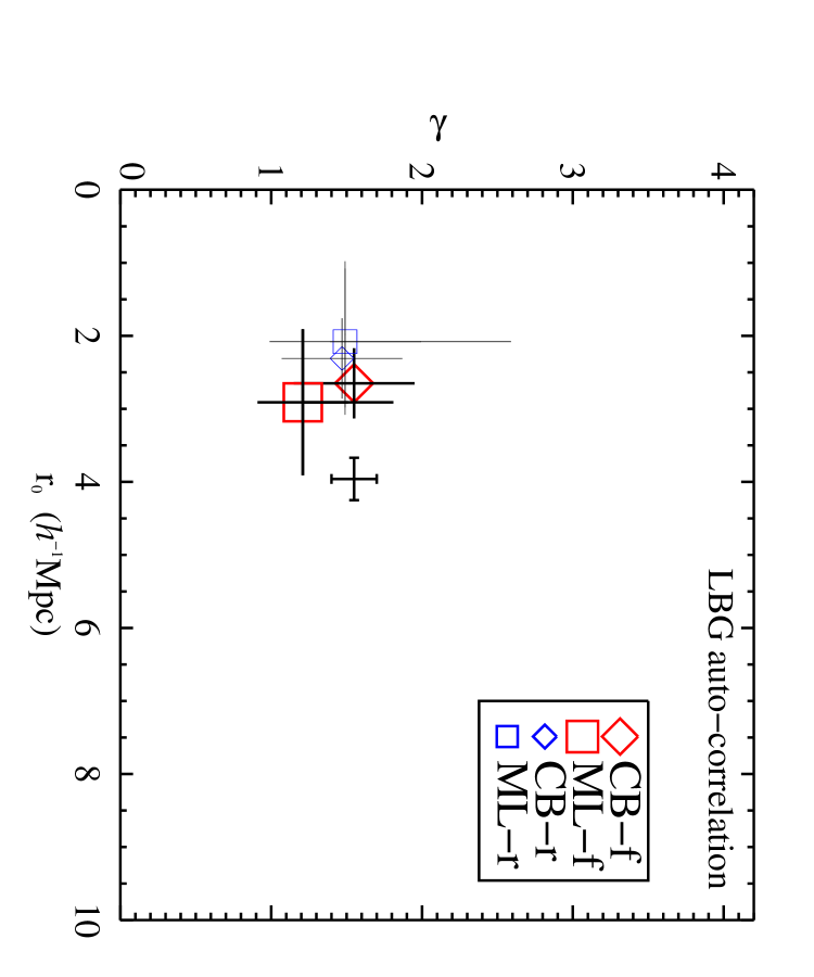
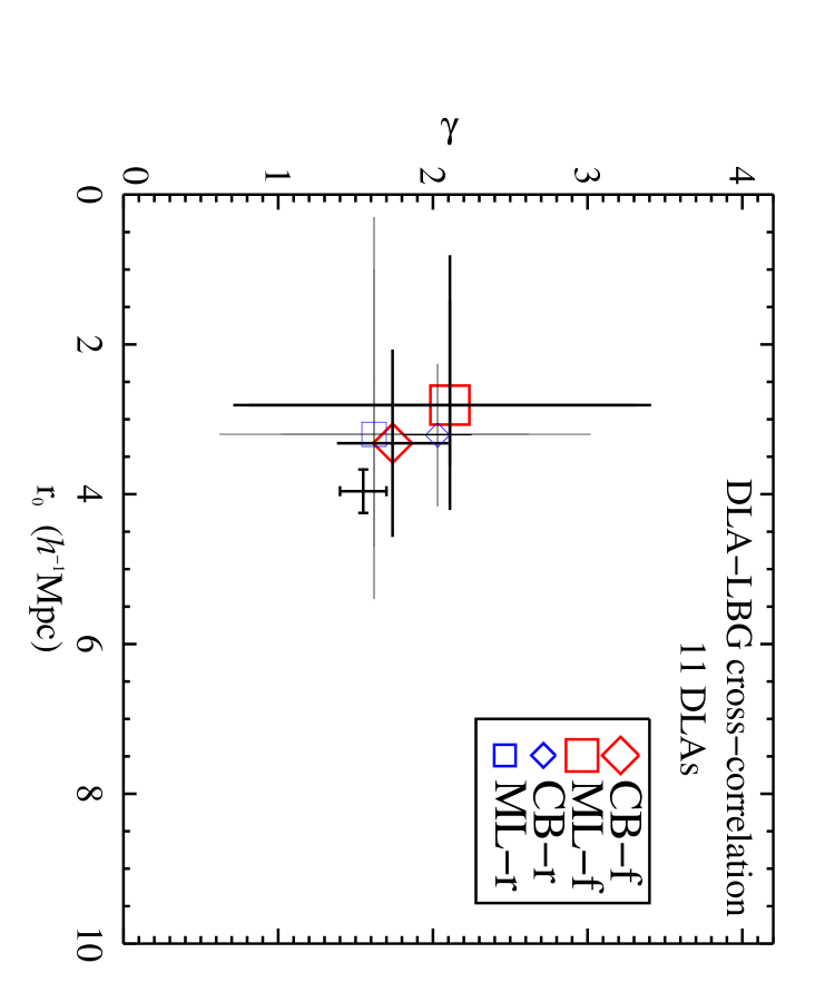
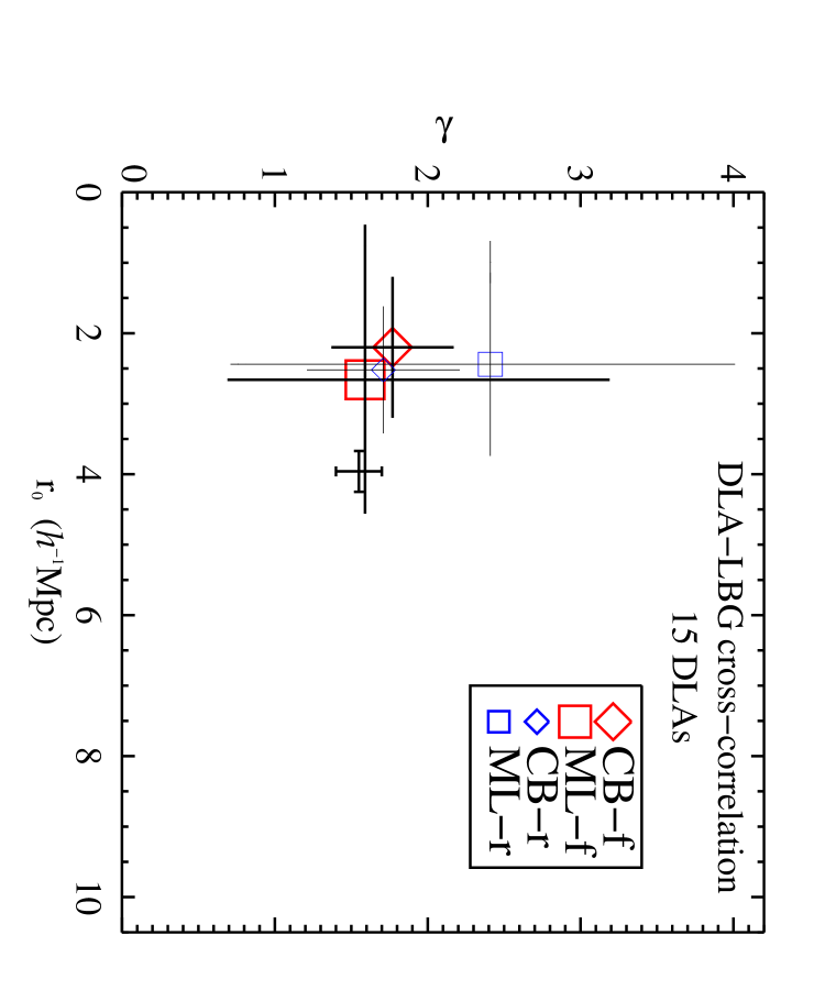
Figure 12: Results summary plots for the LBG auto-correlation and DLA-LBG cross-correlation functions. The best fit values and $1\sigma$ uncertainties are shown for the LBG auto-correlation (upper panel), the DLA-LBG cross-correlation for the 11 DLAs in this survey (center panel), and the full set of 15 DLAs (lower panel) that includes 4 DLAs from the available dataset of Steidel et al. (2003). Large bold symbols indicate the results for the correlation function measurements and small symbols indicate the results for the tests on these measurements. The values for the LBG auto-correlation determined by Adelberger et al. (2003) are shown by the error cross at $r_{0}=3.96,\gamma=1.55$ for comparison. The legend code is as follows: CB = Conventional binning, ML = Maximum likelihood, f = galaxies in the random catalogs have the fixed angular positions of the data, r = galaxies in the random catalogs have random positions.

We used a modified version of the conventional binning technique following the prescription in A03 and measured best fit values and $1\sigma$ uncertainties of $r_{0}=2.65\pm 0.48$ and $\gamma=1.55\pm 0.40$ for the $z\sim 3$ LBG auto-correlation function. These results are in agreement with the previous measurement by A03 when considering that the uncertainties may be underestimated by a factor of $1-2$ (§ 6.1). Applying this technique to the DLA-LBG cross-correlation resulted in best fit values and $1\sigma$ errors of $r_{0}=3.32\pm 1.25$ and $\gamma=1.74\pm 0.36$ for the set of 11 DLAs in our survey and $r_{0}=2.20\pm 0.96$, $\gamma=1.73\pm 0.39$ for the combined set of 15 DLAs that include 4 DLAs from the survey of S03. These results are shown as large (red) diamonds in Figure 12.

Although the above binning technique can produce accurate results, conventional binning techniques in general are dependent on bin size, interval, and bin center. To get around these dependencies, we independently measured the correlation functions using a maximum likelihood technique based on Poisson statistics. This method is bin-independent, makes full use of the data, and is ideal for small datasets. We found maximum likelihood values and $1\sigma$ confidence levels of $r_{0}=2.91^{+1.0}_{-1.0},\gamma=1.21^{+0.6}_{-0.3}$ for the LBG auto-correlation function and $r_{0}=2.81^{+1.4}_{-2.0},\gamma=2.11^{+1.3}_{-1.4}$ and $r_{0}=2.66^{+1.9}_{-2.1},\gamma=1.59^{+1.6}_{-0.9}$ for the DLA-LBG cross-correlation functions for the sets of 11 and 15 DLAs, respectively. The results for both the auto-correlation and the cross-correlation are indicated by large (red) squares in Figure 12.

We tested the effects that the physical constraints of the slitmasks have on the angular component of the correlation function by re-analyzing the data by means of the above two techniques and assigning random angular positions to the random galaxy catalogs instead of the angular positions of the data as was imposed in the original analysis. The test results using the conventional binning technique are shown as small (blue) diamonds in Figure 12 and as small (blue) squares using the maximum likelihood technique.

Furthermore, we discovered a relative spike of five LBGs within $\Delta z=0.015$ of the $z=2.936$ DLA in the field PSS0808+5215 and tested the average DLA-LBG clustering signal in the absence of this DLA. As expected, the amplitude of the clustering was diminished, but the overdensity and form of the correlation function survives and remains in good agreement with the values determined for the complete set of DLAs.

Lastly, we found that two of the six QSOs in the survey spectra lie within $\Delta z=0.0125$ of two of the DLAs. We determine a 1 in 940 chance of this occurring randomly and interpret this to suggest a possible relationship between the distribution of QSOs and DLAs at $z\sim 3$. If found to be a common occurence, the close proximity of QSOs to DLAs could lend insight into the duty-cycle of QSOs and the size and persistence of systems with high Hi column densities near sources of significant ionizing radiation.

It can be seen from Figure 12 that all of the independent methods varying both $r_{0}$ and $\gamma$, and tests of those methods, produce results that are in agreement within their uncertainties. This is also true for the measurements of $r_{0}$ holding $\gamma$ fixed when using all methods (Table 5). The DLA-LBG cross-correlation function, determined from both the set of 11 DLAs in our survey and the combined set of 15 DLAs, exhibits a measurable clustering signal and has best fit parameters in agreement with those of the LBG auto-correlation function. The individual measurements of the DLA-LBG cross-correlation function are only able to measure the DLA galaxy bias to $1-2\sigma$ and we expect to improve this measurement to $\sim 3\sigma$ significance when combining these results with those of our One-Degree Deep survey in progress. When letting $r_{0}$ and $\gamma$ vary, we found that the best fit values and their uncertainties suggest an LBG galaxy bias of $1.5<b_{LBG}<3$ corresponding to an average halo mass of $10^{9.7}<\langle M_{LBG}\rangle<10^{11.6}~{}M_{\odot}$. The DLA galaxy bias determined identically for the 11 DLAs in this survey is $1.3<b_{DLA}<4$ and infers an average DLA mass of $10^{9.7}<\langle M_{LBG}\rangle<10^{12}~{}M_{\odot}$. These values are $0.8<b_{DLA}<4$ and $10^{7.3}<\langle M_{LBG}\rangle<10^{11.7}~{}M_{\odot}$ for the combined set of 15 DLAs. Lastly, we offer the plausible scenario that LBGs reside in the same systems that host DLAs. We identify several pieces of evidence in the literature that support this view. Whatever the true picture, the results from this survey have shed light on the elusive mass of DLAs, their distribution with LBGs, and a possible link between the distribution of QSOs and DLAs at $z\sim 3$.

Table 1: Survey Fields

Field	R.A.(J2000.0)	Dec.(J2000.0)	$z_{QSO}$	$z_{DLA(s)}$	log N(Hi)	$E(B-V)$
	$(h~{}~{}m~{}~{}s)$	$(d~{}~{}m~{}~{}s)$
LBQS0056+0125	00 59 17.62	+01 42 05.30	3.149	2.775	$21.0$	0.03
PKS0336–017	03 39 00.65	$-$01 33 19.20	3.197	3.062	$21.2$	0.14
PSS0808+5215	08 08 49.43	+52 15 14.90	4.450	2.936, 3.113	$20.9$, $20.7$	0.04
PSS0957+3308	09 57 44.50	+33 08 23.00	4.250	3.280	$20.5$	0.01
BRI1013+0035	10 15 48.96	+00 20 19.52	4.381	3.103	$21.1$	0.03
PSS1057+4555	10 57 56.39	+45 55 51.97	4.116	3.050, 3.317	$20.3$ , , $20.3$	0.01
PSS1432+3940	14 32 24.90	+39 40 24.00	4.280	3.272	$21.3$	0.01
PC1643+4631A	16 45 01.09	+46 26 16.44	3.790	3.137	20.7	0.02
JVAS2344+3433	23 44 51.25	+34 33 48.64	3.053	2.908	$21.1$	0.08

Table 2: PSS0808+5215 Cell Counts

$r_{z}$	$h^{-1}$ Mpc	LBGs
0.0025	1.68	2
0.0050	3.36	2
0.0075	5.03	3
0.0100	6.71	3
0.0125	8.38	3
0.0150	10.05	5
⋮	⋮	5
0.0450	29.99	6

Table 3: LBG Auto-Correlation Parameter Summary

Method	$r_{0}$	$\gamma$
Conventional Binning ,	$2.65\pm 0.5$	$1.55\pm 0.4$
Maximum Likelihood	$2.91^{+1.0}_{-1.0}$	$1.21^{+0.6}_{-0.3}$
Tests
Conventional Binning ,	$2.31\pm 0.6$	$1.47\pm 0.4$
Maximum Likelihood	$2.08^{+1.0}_{-1.1}$	$1.49^{+1.1}_{-0.5}$

Table 4: DLA-LBG Cross-Correlation Parameter Summary

Method	11 DLAs	15 DLAs
	$r_{0}$                  $\gamma$	$r_{0}$                  $\gamma$
Conventional Binning ,	$3.32\pm 1.3$   $1.74\pm 0.4$	$2.20\pm 1.0$    $1.77\pm 0.4$
Maximum Likelihood	$2.81^{+1.4}_{-2.0}$       $2.11^{+1.3}_{-1.4}$	$2.66^{+1.9}_{-2.1}$       $1.59^{+1.6}_{-0.9}$
Tests
Conventional Binning ,	$3.21\pm 1.0$   $2.03\pm 0.2$	$2.52\pm 0.9$    $1.71\pm 0.5$
Maximum Likelihood	$3.20^{+2.2}_{-2.9}$        $1.62^{+1.4}_{-1.0}$	$2.44^{+1.3}_{-1.9}$       $2.41^{+1.6}_{-1.7}$

Table 5: Correlation Lengths for $\gamma=1.6$

Method	LBG-LBG	DLA-LBG(11)	DLA-LBG(15)
Conventional Binning ,	$2.72\pm 0.5$	$3.53\pm 1.0$	$2.27\pm 1.0$
Maximum Likelihood	$3.32^{+0.6}_{-0.6}$	$2.93^{+1.4}_{-1.5}$	$2.66^{+1.2}_{-1.3}$
Tests
Conventional Binning ,	$2.40\pm 0.5$	$3.87\pm 1.0$	$2.53\pm 0.8$
Maximum Likelihood	$2.96^{+0.6}_{-0.7}$	$3.20^{+1.5}_{-1.7}$	$2.61^{+1.3}_{-1.5}$

Figure 1: Redshift distribution of the $z>2$ objects detected in this survey binned with $\Delta z=0.2$. The $u^{\prime}$BVRI color selection technique results in a Gaussian distribution of spectroscopically confirmed objects centered at $z=3.02\pm 0.32$.

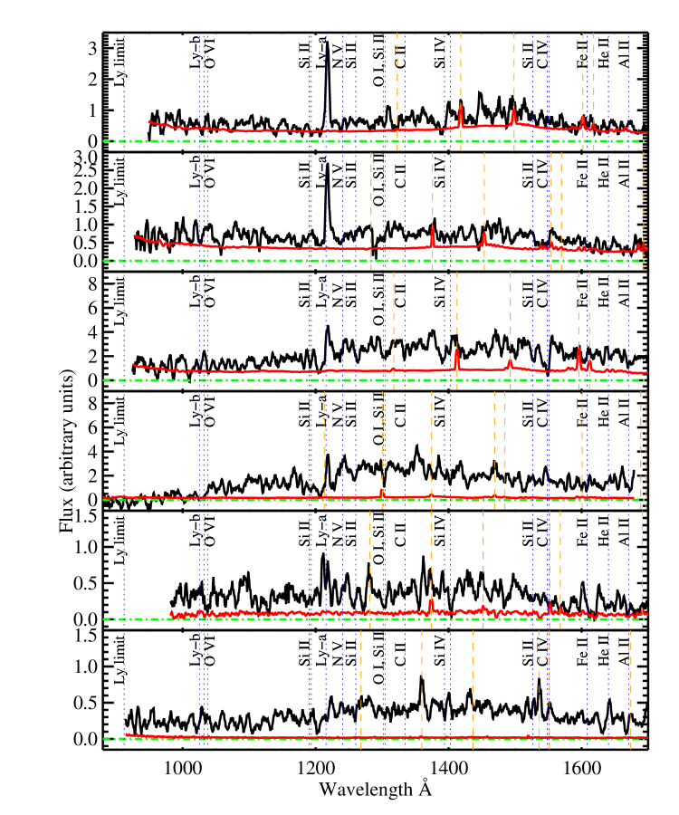
Figure 3: Top to bottom: Objects 0808-0944, 1057-1278, 0808-0377, 0957-1284, 0808-0506, & 0336-0758.

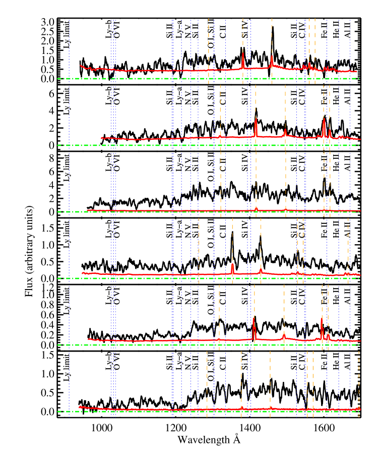
Figure 4: Top to bottom: Objects 1057-3646, 0808-1264, 0808-0269, 0808-0556, 0808-1801, & 1057-0600.

Figure 5: Histogram of the R magnitude distribution of the full $2.6<z<3.4$ LBG sample (hatched) and the LBGs near DLAs (solid). A two-sided Kolmogorov-Smirnov test revealed a high probability that the two cumulative distribution functions are significantly similar

Figure 8: Scatter plot of the LBG auto-correlation from our analysis of the dataset of Steidel et al. (2003). We measured the parameters while varying the logarithmic bin size from $1.125$ to $0.225$ (labeled $1-9$) over a fixed interval of $r_{\theta}\sim 0.04-8h^{-1}$Mpc. The effect of bin size on the correlation values is readily apparent. Although the values appear to converge, smaller samples only allow a few larger bins and may not converge.

Figure 10: Redshift histogram of the $2.6<z<3.4$ LBGs in the PSS0808+5215 field. Objects are binned with $\Delta z=0.03$. The redshifts of the two known DLAs are indicated by the vertical dashed lines.

References

- Adelberger et al. (1998) Adelberger, K. L., Steidel, C. C., Giavalisco, M., Dickinson, M., Pettini, M., & Kellogg, M. 1998, ApJ, 505, 18
- Adelberger et al. (2003) Adelberger, K. L., Steidel, C. C., Shapley, A. E., & Pettini, M. 2003, ApJ, 584, 45
- Adelberger (2004) Adelberger, K. L. 2004, private communication
- Adelberger et al. (2005) Adelberger, K. L., Steidel, C. C., Pettini, M., Shapley, A. E., Reddy, N. A., & Erb, D. K. 2005, ApJ, 619, 697
- Adelberger (2005) Adelberger, K. L. 2005, ApJ, 621, 574
- Bertin & Arnouts (1996) Bertin, E. & Arnouts, S. 1996, A&AS, 117, 393
- Bouché & Lowenthal (2004) Bouché N. & Lowenthal, J. D. 2004, ApJ, 609, 513
- Bouché & Lowenthal (2005) Bouché N., Gardner, J. P., Katz, N., Weinberg, D. H., Davé, R., & Lowenthal, J. D. 2005, ApJ, 628, 89
- Chen & Wolfe (2006) Chen, H. W. & Wolfe, A. M. 2006 in preparation
- Cooke et al. (2005) Cooke, J., Wolfe, A. M., Prochaska, J. X., & Gawiser, E. 2005 ApJ, 621, 596
- Cooke et al. (2006a) Cooke, J., Wolfe, A. M., Gawiser, E., & Prochaska, J. X. 2006 ApJL, 636, 9
- Cooke et al. (2006b) Cooke, J., Wolfe, A. M., Gawiser, E., & Prochaska, J. X. 2006, in prep.
- Croft et al. (1997) Croft, R. A. C., Dalton, G. B., Efstathiou, G., Sutherland, W. J., & Maddox, S. J. 1997, MNRAS, 291, 305
- Daddi et al. (2000) Daddi, E., Cimatti, A., Pozzetti, L., Hoekstra, H., Rottgering, H. J. A., Renzini, A., Zamorani, G., & Mannucci, F. 2000, A&A, 361, 535
- Daddi et al. (2004) Daddi, E., et al. 2004, ApJ, 600, 127
- Davis & Peebles (1983) Davis, M. & Peebles, P. J. E. 1983, ApJ, 267, 465
- Foucaud et al. (2003) Foucaud, S., McCracken, H. J., Le Fèvre, O., Arnouts, S., Brodwin, M., Lilly, S. J., Crampton, D., & Mellier, Y. 2003, A&A, 409, 835
- Gawiser et al. (2001) Gawiser, E., Wolfe, A. M., Prochaska, J. X., Lanzetta, K. M., Yahata, N., & Quirrenbach, A. 2001, ApJ, 562, 628
- Giavalisco & Dickinson (2001) Giavalisco, M. & Dickinson, M. 2001, ApJ, 550, 177
- Hawkins et al. (2003) Hawkins, E., Maddox, S., Cole, S., Lahav, O., Madgwick, D., Norberg, P., Peacock, J. A. et al. 2003, MNRAS, 346, 78
- Kashikawa et al. (2005) Kashikawa, N., Yoshida, M., Shimasaku, K., Nagashima, M., Yahagi, H., Ouchi, M., Matsuda, Y., Malkan, M, A., Doi, M., Iye, M., Ajiki, M., Akiyama, M., Ando, H., Aoki, K., Furusawa, H., Hayashino, T., Iwamuro, F., Karoji, H., Kobayashi, N., Kodaira, K., Kodama, T., Komiyama, Y., Miyazaki, S., Mizumoto, Y., Morokuma, T., Motohara, K., Murayama, T., Nagao, T., Nariai, K., Ohta, K., Okamura, S., Sasaki, T., Sato, Y., Sekiguchi, K., Shioya, Y., Tamura, H., Taniguchi, Y., Umemura, M., Yamada, T., & Yasuda, N. 2006, ApJ, 637, 631
- Kauffmann (1996) Kauffmann, G. 1996, MNRAS, 281, 475
- COSMIC; Kells et al. (1998) Kells, W., Dressler, A., Sivaramakrishnan, A., Carr, D., Koch, E., Epps, H., Hilyard, D., & Pardeilhan, G. 1998, PASP, 110, 1487
- Kerscher et al. (2000) Kerscher, M., Szapudi, I., & Szalay, A. S. 2000, ApJ, 535, 13
- Landy & Szalay (1993) Landy, S. D. & Szalay, A. S. 1993, ApJ, 412, 64
- Lowenthal et al. (1997) Lowenthal, J. D. et al. 1997, ApJ, 481, 673
- Lu et al. (1998) Lu, Limin; Sargent, W. L. W., Barlow, T. A. 1998, AJ, 115, 55
- Maller et al. (2001) Maller, A. H., Prochaska, J. X., Somerville, R. S., & Primack, J. R. 2001, MNRAS, 326, 1475
- McCarthy et al. (2001) McCarthy, P. J., Carlberg, R. G., Chen, H.-W., Marzke, R. O., Firth, A. E., Ellis, R. S., Persson, S. E., McMahon, R. G., Lahav, O., Wilson, J., Martini, P., Abraham, R. G., Sabbey, C. N., Oemler, A., Murphy, D. C., Somerville, R. S., Beckett, M. G., Lewis, J. R., & MacKay, C. D. 2001, ApJ, 560, 131
- McCarthy et al. (2004) McCarthy, P. J., Le Borgne, D., Crampton, D., Chen, H-W., Abraham, R. G., Glazebrook, K., Savaglio, S., Carlberg, R. G., Marzke, R. O., Roth, K., Jørgensen, I., Hook, I., Murowinski, R., & Juneau, S. 2004, ApJ, 614, 9
- Mo et al. (1998) Mo, H. J., Mao, S., & White, S. D. M. 1998, MNRAS, 295, 319
- Sheth, et al. (2001) Sheth, R. K., Mo, H. J., & Tormen, G. 2001, MNRAS, 323, 1
- Møller et al. (2002) Møller, P., Warren, S. J., Fall, S. M., Fynbo, J. P. U., & Jakobsen, P. 2002, ApJ, 574, 51
- Møller et al. (2004) Møller, P., Fynbo, J. P. U., & Fall 2004, ApJ, 422, 33
- Mullis et al. (2004) Mullis, C. R., Henry, J. P., Gioia, I. M., B hringer, H., Briel, U. G., Voges, W., & Huchra, J. P. 2004, ApJ, 617, 192
- Mullis (2005) Mullis, C. R. 2005, private communication
- Nagamine et al. (2004a) Nagamine, K., Springel, V., & Hernquist, L. 2004, MNRAS, 348, 421
- Nagamine et al. (2004b) Nagamine, K., Springel, V., & Hernquist, L. 2004, MNRAS, 348, 435
- Nagamine et al. (2006) Nagamine, K., Wolfe, A. M., Springel, V., & Hernquist, L. 2006, MNRAS, submitted
- LRIS; Oke et al. (1995) Oke, J. B., Cohen, J. G., Carr, M., Cromer, J., Dingizian, A., Harris, F. H., Labrecque, S., Lucinio, R., Schaal, W., Epps, H., & Miller, J. 1995, PASP, 107, 375
- Ouchi et al. (2004) Ouchi, M., Shimasaku, K., Okamura, S., Furusawa, H., Kashikawa, N., Ota, K., Doi, M., Hamabe, M., Kimura, M., Komiyama, Y., Miyazaki, M., Miyazaki, S., Nakata, F., Sekiguchi, M., Yagi, M. & Yasuda, N. 2004, ApJ, 611, 685
- Peebles (1980) Peebles, P. J. E. 1980 The Large-Scale Structure of the Universe, Princeton, N.J., Princeton University Press
- Péroux et al (2001) Péroux, C., Storrie-Lombardi, L. J., McMahon, R. G., Irwin, M., Hook, I. M. 2001, AJ, 121, 1799
- Pettini et al. (2000) Pettini, M., Steidel, C. C., Adelberger, K. L., Dickinson, M., & Giavalisco, M. 2000, ApJ, 528, 96
- Pettini et al. (2001) Pettini, M., Shapley, A. E., Steidel, C. C., Cuby, J-G., Dickinson, M., Moorwood, A. F. M., Adelberger, K. L., & Giavalisco, M. 2001, ApJ, 554, 981
- Pettini et al. (2002) Pettini, M., Rix, S. A., Steidel, C. C., Adelberger, K. L., Hunt, M. P., & Shapley, A. E. 2002, AJ, 569, 742
- Porciani & Giavalisco (2002) Porciani, C. & Giavalisco, M. 2002, ApJ, 565, 24
- Press et al. (1992) Press, W. H., Flannery, B. P., Teukolsky, S. A. & Vetterling, W. T. 1992, “Numerical Recipes in C”, (Cambridge: Cambridge University Press)
- Prochaska & Wolfe (1997) Prochaska, J. X. & Wolfe, A. M. 1997, ApJ, 487, 73
- Prochaska & Wolfe (1998) Prochaska, J. X. & Wolfe, A. M. 1998, ApJ, 507, 113
- Prochaska et al. (2001) Prochaska, J. X., Wolfe, A. M., Tytler, D., Burles, S., Cooke, J., Gawiser, E., Kirkman, D., O’Meara, J. M., & Storrie-Lombardi, L. 2001, ApJS, 137, 21
- Prochaska et al. (2003) Prochaska, J. X., Gawiser, E., Wolfe, A. M., Cooke, J., Gelino, D. 2003, ApJS, 147, 227
- Prochaska, Herbert-Fort, & Wolfe (2005) Prochaska, J. X., Herbert-Forte, S., & Wolfe, A. M. 2005, ApJ, 635, 123
- Quadri et al. (2006) Quadri, R., van Dokkum, P., Gawiser, E., Franx, M., Marchesini, D., Lira, P., Rudnick, G, Herrera, D., Maza, J., Kriek, M., Labbé, I., & Francke, H. 2006, arXiv:astro-ph/0606330
- Roche et al. (1999) Roche, N., Eales, S. A., Hippelein, H., & Willott, C. J. 1999, MNRAS, 306, 538
- Schaye (2001) Schaye, J. 2001, ApJ, 559, 1
- Schneider et al. (1991) Schneider, D. P., Schmidt, M., Gunn, J. E. 1991, AJ, 101, 2004
- Shapley et al. (2003) Shapley, A. E., Steidel, C. C., Adelberger, K. L., & Pettini, M. 2003, ApJ, 588, 65
- Steidel et al. (1996a) Steidel, C. C., Giavalisco, M., Pettini, M., Dickinson, M., & Adelberger, K. L. 1996, ApJ, 462L, 17
- Steidel et al. (1996b) Steidel, C. C., Giavalisco, M., Dickinson, M., & Adelberger, K. L. 1996, AJ, 112, 352
- Steidel et al. (1998) Steidel, C. C., Adelberger, K. L., M., Dickinson, Giavalisco, M., Pettini, M., & Kellogg, M. 1998, ApJ, 492, 428
- Steidel et al. (2003) Steidel, C. C., Adelberger, K. L., Shapley, A. E., Pettini, M., Dickinson, M., & Giavalisco, M. 2003, ApJ, 592, 728
- Storrie-Lombardi & Wolfe (2000) Storrie-Lombardi, L. & Wolfe, A. M. 2000, ApJ, 543, 552
- Wolfe et al. (1986) Wolfe, A. M., Turnshek, D. A., Smith, H. E., & Cohen, R. D. 1986, ApJS, 61, 249
- Wolfe et al. (1995) Wolfe, A. M., Lanzetta, K. M., Foltz, C. B., & Chaffee, F. H. 1995, ApJ, 454, 698
- Wolfe & Prochaska (2000a) Wolfe, A. M. & Prochaska, J. X. 2000, ApJ, 545, 591
- Wolfe & Prochaska (2000b) Wolfe, A. M. & Prochaska, J. X. 2000, ApJ, 545, 603
- Wolfe et al. (2003) Wolfe, A. M., Prochaska, J. X., & Gawiser, E. 2003, ApJ, 593, 215
- Wolfe et al. (2005) Wolfe, A. M., Gawiser, E. & Prochaska, J.X. 2005, ARA&A 43, 861