Dark energy and curvature from a future baryonic acoustic oscillation survey using the Ly$\alpha$ forest 

Abstract

We explore the requirements for a Lyman-$\alpha$ forest survey designed to measure the angular diameter distance and Hubble parameter at $2\lesssim z\lesssim 4$ using the standard ruler provided by baryonic acoustic oscillations (BAO). The goal would be to obtain a high enough density of sources to probe the three-dimensional density field on the scale of the BAO feature. A percent-level measurement in this redshift range can almost double the Dark Energy Task Force Figure of Merit, relative to the case with only a similar precision measurement at $z\sim 1$, if the Universe is not assumed to be flat. This improvement is greater than the one obtained by doubling the size of the $z\sim 1$ survey, with Planck and a weak SDSS-like $z=0.3$ BAO measurement assumed in each case. Galaxy BAO surveys at $z\sim 1$ may be able to make an effective Ly$\alpha$ forest measurement simultaneously at minimal added cost, because the required number density of quasars is relatively small. We discuss the constraining power as a function of area, magnitude limit (density of quasars), resolution, and signal-to-noise of the spectra. For example, a survey covering 2000 sq. deg. and achieving $S/N=1.8$ per Å at $g=23$ ($\sim 40$ quasars per sq. deg.) with an $R\gtrsim 250$ spectrograph is sufficient to measure both the radial and transverse oscillation scales to 1.4% from the Ly$\alpha$ forest (or better, if fainter magnitudes and possibly Lyman-break galaxies can be used). At fixed integration time and in the sky-noise-dominated limit, a wider, noisier survey is generally more efficient; the only fundamental upper limit on noise being the need to identify a quasar and find a redshift. Because the Ly$\alpha$ forest is much closer to linear and generally better understood than galaxies, systematic errors are even less likely to be a problem.

I Introduction

The existence of new physics that causes the Universe to accelerate at late times is well established, both by observations of Type Ia supernovas (Knop et al., 2003; Riess et al., 2004; Astier et al., 2006) and by combinations of other observables (Seljak et al., 2006). The focus now is on probing the properties of the acceleration, most commonly thought to be caused by dark energy, a substance we know almost nothing about except that it must have negative pressure. We often parameterize dark energy by the equation of state, $w=p/\rho$, where $p$ is the pressure and $\rho$ the density ($w=-1$ for a cosmological constant). In general, $w$ can be time-dependent (Ratra and Peebles, 1988).

Acoustic oscillations before recombination lead to a feature in the matter correlation function at the scale of the sound horizon at decoupling (Peebles and Yu, 1970; Sunyaev and Zeldovich, 1970; Doroshkevich et al., 1978). CMB observations pin this scale at $143\pm 4$ Mpc (Page et al., 2003). Recently, Eisenstein et al. (2005) detected the expected enhancement (at $>3\sigma$) in the correlation of the Sloan Digital Sky Survey (SDSS) Luminous Red Galaxies (LRGs). In coming years, precision measurements of the BAO feature will be used as a standard ruler to probe the equation of state of dark energy (Eisenstein et al., 1998; Eisenstein and Hu, 1998; Cooray et al., 2001; Eisenstein, 2003; Blake and Glazebrook, 2003; Linder, 2003; Seo and Eisenstein, 2003; Matsubara, 2004; Glazebrook and Blake, 2005; Glazebrook et al., 2005; Amendola et al., 2005; Blake and Bridle, 2005; Blake et al., 2006; Dolney et al., 2006).

We define the usual cosmological parameters in addition to $w$: The scale factor is $a=1/(1+z)$, with Hubble parameter $H(z)=\dot{a}/a$ with $H(0)=H_{0}=h~{}100~{}{\rm km~{}s^{-1}Mpc^{-1}}$. The baryon density is $\omega_{b}=\Omega_{b}h^{2}$ where $\Omega_{b}=\rho_{b}/\rho_{c}$ is the fraction of the critical density, $\rho_{c}=3H_{0}^{2}/8\pi G$, in baryons. The matter density is $\omega_{m}=\Omega_{m}h^{2}$, where $\Omega_{m}$ is the fraction of the critical density in baryons plus cold dark matter. The fraction of the critical density in dark energy is $\Omega_{w}$. The curvature is parameterized by $\Omega_{k}=1-\Omega_{m}-\Omega_{w}$. The primordial power spectrum is parameterized by its amplitude $A$ and power law index, $n_{s}$ (we will not use tensors or running of the spectral index in this paper). The Thompson scattering optical depth to the CMB surface of last scattering is $\tau$. We will sometimes use $\theta_{s}$ at the CMB last scattering redshift, defined below in Eq. (2), as a free parameter in place of $h$. We measure $\theta_{s}$ in degrees so a typical value is 0.6.

In general, the quantities measured most directly in a BAO study are

$$v_{s}(a)=H(a)~{}s~{}a$$ (1)

in the radial direction and

$$\theta_{s}(a)=\frac{s~{}a}{D_{A}(a)}$$ (2)

in the transverse direction, where $s$ is the comoving sound horizon at decoupling (Hu, 2005), and $D_{A}(a)$ is the angular diameter distance. For flat models, $D_{A}(a)/a=r(a)$ and $\theta_{s}(a)=s/r(a)$ with

$$r(a)=\int_{a}^{1}\frac{c}{a^{\prime 2}H(a^{\prime})}da^{\prime}~{}.$$ (3)

For curved models,

$$(1+z)~{}D_{A}(a)=R~{}\sinh\left[\frac{r(a)}{R}\right]$$ (4)

with

$$R=\frac{c}{H_{0}\sqrt{\Omega_{k}}}~{}.$$ (5)

Finally,

$$s=\int_{0}^{a_{r}}\frac{c_{s}(a)}{a^{2}H(a)}da$$ (6)

where $a_{r}\simeq 1/1090$ is the recombination redshift ((Hu, 2005) gives a useful fitting formula for $a_{r}$’s relatively small parameter dependence), and $c_{s}(a)=c/\sqrt{3\left(1+3\rho_{b}/4\rho_{\gamma}\right)}$, where $\rho_{\gamma}$ is the photon density.

In this paper, we discuss the possibility of measuring the BAO feature in a Ly$\alpha$ forest survey (see also White (2003)). The acoustic scale $143~{}{\rm Mpc}$ corresponds to $\sim 1.3$ degrees on the sky at $z\sim 2.8$, our typical mean redshift. On this large scale, the clustering of the absorption can be assumed to follow a linear bias model in a way analogous to galaxies. This has been studied in simulations by McDonald (2003). The primary difference from galaxy surveys is in how the density field is sampled on relatively small scales. With galaxies, we observe a collection of discrete points, which we believe are a Poisson sampling of the underlying density field. For the Ly$\alpha$ forest, we observe a collection of skewers through the density field, obtaining a detailed picture along the skewers, but no information in between. The reader who is uncomfortable with this should consider that they are probably perfectly comfortable constructing a density field from the ultimately zero dimensional galaxy sampling – in the forest we not only have a fully one-dimensional field, we even measure a continuous value rather than the discrete presence or absence of a galaxy. For galaxies there is intrinsic noise due to the Poisson sampling, while for the Ly$\alpha$ forest there is intrinsic aliasing-like noise due to the discrete transverse sampling. As we will show, if the sampling of the Ly$\alpha$ forest was only zero dimensional, this noise would take approximately the same white (uncorrelated) form as the galaxy noise. Of course, the Ly$\alpha$ forest also has the advantage of being sensitive to the near-mean-density intergalactic medium (IGM), rather than the highly non-linear positions of galaxies, so we can more confidently back up our assumptions with near-first-principles calculations. This is not to say that the Ly$\alpha$ forest is decisively superior to galaxies as a high-z BAO probe. Ultimately, both should work, and the resource requirements to conduct an equivalent survey are the most important factor in deciding which is better.

Computing the expected errors obtainable from the Ly$\alpha$ forest as a function of survey parameters is the main aim of this paper. In §II we describe our basic method for estimating obtainable errors on $\theta_{s}$ and $v_{s}$. Then in §III we give the results. Finally, in §IV, we discuss the usefulness for constraining dark energy and curvature of a measurement of $\theta_{s}(z\sim 3)$ and $v_{s}(z\sim 3)$.

II Setting up the calculation

In this section we discuss our method for estimating the constraining power of future surveys. First, in §II.1, we define the parameters that describe the survey configuration. Then, in §II.2, we explain our Fisher matrix calculations. Finally, in §II.3 we explain our theoretical model for the Ly$\alpha$ forest power spectrum.

II.1 Assumed data set

We assume a square survey with area $A$ and comoving number density of quasars $n_{q}$. We usually ignore evolution across the redshift extent of the survey, e.g., $n_{q}$ is the density at the central redshift. One would of course need to consider evolution in an analysis of real data, but, as we will show, the resulting error bars will not be increased relative to a Fisher matrix estimate that ignores evolution. $n_{q}$ will be a function of the central redshift and magnitude limit of the survey, based on the luminosity function, $\frac{dn_{q}}{dm}(z)$, taken from Jiang et al. (2006). Beyond setting $n_{q}$, the luminosity function is relevant for setting the distribution of noise levels in spectra. We assume that the survey probes the forest in the observed wavelength range $\lambda_{{\rm min}}<\lambda<\lambda_{{\rm max}}$, which we translate to $z_{\rm min}$ and $z_{\rm max}$ using $\lambda=\lambda_{\alpha}(1+z)$ (with $\lambda_{\alpha}=1216$Å). The central redshift is just $(z_{\rm min}+z_{\rm max})/2$. We assume the usable rest wavelength range in a single spectrum is $\lambda_{{\rm rest,min}}<\lambda_{{\rm rest}}<\lambda_{{\rm rest,max}}$, generally using $\lambda_{{\rm rest,min}}=1041$Å and $\lambda_{{\rm rest,max}}=1185$Å (this is very conservative - one could probably extend the baryonic oscillation analysis into the Lyman-$\beta$-influenced region without much difficulty). We will occasionally call the length in the IGM probed by a single line of sight $L_{q}$ ($\sim 330\,h^{-1}\,{\rm Mpc}$ for these limits). The spectrograph is assumed to have rms resolution $\sigma_{R}$ (${\rm FWHM}=2.355~{}\sigma_{R}=\lambda/R$). Spectral pixels are assumed to have full width $l_{p}=\sigma_{R}$. We assume rms noise per pixel $\sigma_{N}$, in units of the mean transmitted flux level in the forest.

II.2 Fisher matrix calculation

We estimate the errors on parameters $p_{i}$, obtainable using a future survey, to be $(F^{-1})_{ii}$, where $F_{ij}$ is the Fisher matrix (Tegmark et al., 1997):

$$F_{ij}=\left<\frac{\partial^{2}\mathcal{L}}{\partial p_{i}\partial p_{j}}\right>~{},$$ (7)

with

$$2\mathcal{L}=\ln\det\mathbf{C}+\mathbf{\delta}^{T}\mathbf{C}^{-1}\mathbf{\delta}+{\rm constant}$$ (8)

for a real mean zero Gaussian vector ${\mathbf{\delta}}$ of data points with covariance matrix $C_{ij}({\mathbf{p}})=\left<\delta_{i}\delta_{j}\right>$. From Tegmark et al. (1997) (and references therein), we have

$$F_{ij}=\frac{1}{2}{\rm Tr}\left(\mathbf{C}^{-1}\frac{\partial\mathbf{C}}{\partial p_{i}}\mathbf{C}^{-1}\frac{\partial\mathbf{C}}{\partial p_{j}}\right)~{}.$$ (9)

We could always take $\delta_{i}$ to be individual pixels in spectra and evaluate Eq. (9) by brute force; however, this calculation would quickly become difficult. For example, our fiducial survey would have about 40 million pixels. While we could probably reduce this number enough to produce a reasonably invertible covariance matrix by scaling up from a much smaller survey and pushing the pixel size and angular sampling to just barely resolve the BAO feature, it is better to look for a more efficient method.

Methods for applying the Fisher matrix formalism to a BAO survey using galaxies are well-developed (Seo and Eisenstein, 2003). Counts of galaxies (say, in cells smaller than the scale of interest) are the density field of interest, but the calculations are done in Fourier space. Assuming an approximately uniform selection function, the covariance matrix of Fourier modes is approximately diagonal if the wavenumber $k_{j}$ is discretized in bands of width $2\pi/L_{j}$, where $L_{j}$ is the survey width in direction $j$. The covariance matrix of the real and imaginary parts of Fourier modes is simply $C_{ii}({\mathbf{p}})=\frac{1}{2}\left[P_{g}({\mathbf{k}}_{i},{\mathbf{p}})+P_{N}\right]$, where $P_{g}$ is the redshift-space galaxy power spectrum and $P_{N}=1/\bar{n}_{g}$ is the Poisson noise power for mean galaxy density $\bar{n}_{g}$. Simple formulas for the Fisher matrix as an integral over $k$ can be derived.

The Ly$\alpha$ forest is slightly more complicated. Here, the quasar lines of sight going through some volume are approximately random. Our density estimate for the volume is not determined by the number of lines of sight probing it, but rather by some average of the absorption in those lines of sight. Working toward a covariance matrix of Fourier modes, we will take $\delta_{i}$ in the Fisher matrix to be the Fourier modes of the weighted density field

$$\delta({\mathbf{x}})=\frac{w({\mathbf{x}})}{\bar{w}}[\delta_{F}({\mathbf{x}})+\delta_{N}({\mathbf{x}})]~{}.$$ (10)

where $\delta_{F}({\mathbf{x}})=\delta_{F}(z,{\mathbf{\theta}})=F(z,{\mathbf{\theta}})/\bar{F}-1$ where $F=\exp(-\tau)$ is the transmitted flux fraction in the forest, $\delta_{N}({\mathbf{x}})$ is the spectral noise, $w({\mathbf{x}})$ is the weight at ${\mathbf{x}}$, and $\bar{w}$ is the mean weight. We will not specify the weights at this point, but generally they should depend on pixel noise variance. The relevant quantities are all defined over fully three-dimensional space – if some location is not probed by a quasar line of sight, the weight is simply zero. The correlation of Fourier modes of $\delta({\mathbf{x}})$ is

$$\left<\delta_{\mathbf{k}}\delta_{{\mathbf{k}}^{\prime}}\right>=\int d{\mathbf{x}}~{}d{\mathbf{x}}^{\prime}\exp(i{\mathbf{k}}\cdot{\mathbf{x}}+i{\mathbf{k}}^{\prime}\cdot{\mathbf{x}}^{\prime})~{}\left[\xi_{F}({\mathbf{x}}-{\mathbf{x}}^{\prime})+\xi_{N}({\mathbf{x}},{\mathbf{x}}^{\prime})\right][1+\delta_{w}({\mathbf{x}})][1+\delta_{w}({\mathbf{x}}^{\prime})]~{},$$ (11)

defining $\delta_{w}({\mathbf{x}})=w({\mathbf{x}})/\bar{w}-1$, and $\xi_{X}\left({\mathbf{x}},{\mathbf{x}}^{\prime}\right)=\left<\delta_{X}({\mathbf{x}})\delta_{X}({\mathbf{x}}^{\prime})\right>$.

We do not know the weights in advance, because they depend on the random quasar locations and luminosities. We can, however, evaluate the average of the weight term, which should give us a good estimate of the constraining power of the survey (for a typical survey of $\sim 10000$ quasars, a quantity measured from a single realization should not deviate much from the average quantity). Our pixel weights will be approximately uncorrelated in the transverse directions, and perfectly correlated in the radial direction (for simplicity we are assuming pixels in the same spectrum have the same noise). For a continuous white noise field, $\xi({\mathbf{x}})=P~{}\delta^{D}({\mathbf{x}})$, where $P$ is the constant power spectrum of the field. This gives

$$\left<\delta_{w}({\mathbf{x}})\delta_{w}({\mathbf{x}}^{\prime})\right>=P_{w}^{\rm 2D}\delta^{D}({\mathbf{x}}_{\perp})$$ (12)

where $P_{w}^{\rm 2D}$ is the power spectrum of $\delta_{w}$ in the two angular directions. This means

$$\left<\delta_{\mathbf{k}}\delta_{{\mathbf{k}}^{\prime}}\right>\simeq(2\pi)^{3}\delta^{D}({\mathbf{k}}+{\mathbf{k}}^{\prime})\left[P_{F}({\mathbf{k}})+P_{F}^{\rm 1D}(k_{\parallel})P_{w}^{\rm 2D}+P^{\rm eff}_{N}\right]~{},$$ (13)

where $P_{F}^{\rm 1D}(k_{\parallel})$ is the usual 1D flux power spectrum measured along single lines of sight, and $P^{\rm eff}_{N}$ is the weighted noise power, which does not separate like the other term because the weights depend on the noise amplitude. Note that modes with different ${\mathbf{k}}$ are still approximately uncorrelated.

We now need to evaluate the $P_{w}^{\rm 2D}$ term. The low-k power spectrum for a pixelated white noise field is $P=\sigma^{2}v$, where $\sigma^{2}$ is the pixel variance and $v$ is the pixel volume (in a general sense, i.e., here the volume is actually an area because we are working in two dimensions). As a computational device, let us imagine pixelating the transverse directions into small cells of angular width $l$ (we will eventually take $l\rightarrow 0$). Then, $P_{w}^{\rm 2D}=\sigma_{w}^{2}l^{2}$, with $\sigma^{2}_{w}=\left<w^{2}\right>/\bar{w}^{2}-1$. The noise in a spectrum is a function of the apparent magnitude of the quasar, so the mean weight is

$$\bar{w}=\int_{-\infty}^{m_{\rm max}}dm\frac{dn_{q}}{dm}~{}L_{q}~{}l^{2}~{}w(m)\equiv l^{2}L_{q}I_{1}~{}.$$ (14)

Note that $L_{q}l^{2}dn_{q}/dm$ is the probability that a given small volume of the IGM will be probed by a line of sight to a quasar of apparent magnitude $m$. Similarly,

$$\left<w^{2}\right>=\int_{-\infty}^{m_{\rm max}}dm\frac{dn_{q}}{dm}~{}L_{q}~{}l^{2}~{}w^{2}(m)\equiv l^{2}L_{q}I_{2}~{}.$$ (15)

Therefore, in the limit $l\rightarrow 0$,

$$P^{\rm 2D}_{w}=\frac{I_{2}}{I_{1}^{2}L_{q}}$$ (16)

A similar calculation leads to

$$P^{\rm eff}_{N}=\frac{I_{3}l_{p}}{I_{1}^{2}L_{q}}$$ (17)

where

$$I_{3}\equiv\int_{-\infty}^{m_{\rm max}}dm\frac{dn_{q}}{dm}~{}\sigma_{N}^{2}(m)w^{2}(m)~{}.$$ (18)

Note that $I_{1}L_{q}/l_{p}$ is something like an effective 3D pixel density (recall that $l_{p}$ is the pixel width), while $I_{3}/I_{1}$ is the effective noise variance in these pixels.

We take the weights to have the simple Feldman, Kaiser, & Peacock (hereafter FKP) inverse variance form Feldman et al. (1994),

$$w(m)=\frac{P_{S}/P_{N}(m)}{1+P_{S}/P_{N}(m)}~{},$$ (19)

where $P_{S}$ is the typical signal power and $P_{N}({\mathbf{x}})=P_{N}[m({\mathbf{x}})]$ is the noise power level associated with the noise level at ${\mathbf{x}}$ (if there is no quasar probing ${\mathbf{x}}$, this level is infinite so the weight is zero). The numerator is chosen to make $w({\mathbf{x}})=1$ in the low noise limit. There is a subtlety at this point in that $P_{N}(m)$ is not unambiguously defined. If quasars were evenly distributed in angle, and all had the same magnitude, then clearly $P_{N}=\sigma_{N}^{2}l_{p}/n_{q}L_{q}$. The only reasonable possibility in the realistic case seems to be to take $P_{N}(m)=\sigma^{2}_{N}(m)l_{p}/I_{1}L_{q}=\sigma^{2}_{N}(m)/n_{p}^{\rm eff}$, where $n_{p}^{\rm eff}$ is the effective pixel density. Note the similarity to galaxy shot noise: if the overall mean density of galaxies is $\bar{\bar{n}}_{g}$, and the mean at point ${\mathbf{x}}$ is $\bar{n}_{g}({\mathbf{x}})$, then the Poisson-noise variance at point ${\mathbf{x}}$ is $\sigma_{P}^{2}=\bar{\bar{n}}_{g}/\bar{n}_{g}({\mathbf{x}})$ for cells with volume $1/\bar{\bar{n}}_{g}$, and the noise factor in the usual FKP weights is $\sigma^{2}_{P}({\mathbf{x}})/\bar{\bar{n}}_{g}$ (recall that our $m$ dependence is equivalent to ${\mathbf{x}}$ dependence). Since $n_{p}^{\rm eff}$ and the weights are mutually dependent, we determine them using a few iterations. After some experimentation showing that the results are not very sensitive to the choice of $P_{S}$, we take the shortcut of using one constant for $P_{S}$: the total flux power in the central model at $k=0.07\,h\,{\rm Mpc}^{-1}$, $\mu=k_{\parallel}/k=0.5$, including the aliasing term (which is formally signal, although in practice it acts as noise).

There are a couple of loose ends in this derivation. First, we are going to assume that, having computed the power spectrum, i.e., the covariance matrix of Fourier modes, averaged over realizations of the weights, we can simply proceed with the calculation of the constraining power of a survey as if this were the exact power spectrum; however, the averages of the covariance matrix of power measurements, or of the Fisher matrix, are not necessarily the same as what one computes from the averaged power spectrum. Ideally we would only average at the last possible point in the computation (remember, the Fisher matrix is already an average of the derivatives of the likelihood function over all possible future data sets). Unfortunately, without the assumption that the Fourier modes are uncorrelated, we are stuck with the problem of inverting a very large covariance matrix, and now we would need to do it many times to average over realizations. To investigate this problem, we computed the average covariance matrix of the power spectrum measurements and found that the new terms are suppressed by a factor of the number of quasars in the survey (i.e., the ratio of the area of the survey to the area per line-of-sight) relative to the standard terms, as long as the second term in Eq. (13) is not much larger than the first. This will be the case any time the BAO measurement is possible, so it seems we are safe to ignore this issue. Second, with no Nyquist frequency for a randomly sampled survey, it is not clear at what k we should stop counting modes. This is worrisome because we will find that our constraining power will continue to increase somewhat beyond the transverse Nyquist frequency associated with the effective mean density of lines of sight. This means that we are using more Fourier modes than we have data points, and the assumption that they are uncorrelated probably has to break down somehow, e.g., due to an accumulation of small correlations. To be conservative, we only use modes with $k$ less than the Nyquist frequency associated with the effective mean density. We also eliminate modes with $k>0.5\,h\,{\rm Mpc}^{-1}$ (relevant only in the radial direction). To allow for continuum fitting, we drop all the modes having the first $2N_{\rm q,los}$ discrete values of $k_{\parallel}$, counting both positive and negative $k_{\parallel}$, where $N_{\rm q,los}$ is the number of spectra it takes to cover the redshift range of our survey (the first 5 values of $k_{\parallel}$ for our standard survey). These last two cuts make no noticeable difference in the results.

We note for the future that one would probably perform the data analysis using a more sophisticated maximum likelihood method (Tegmark et al., 1997), but this FKP-like method should be good enough for the Fisher matrix error estimate.

II.3 Three-dimensional Ly$\alpha$ forest power spectrum

Missing from the discussion so far has been any mention of how we predict the Ly$\alpha$ forest power spectrum and its parameter dependence that is needed for the Fisher matrix calculation. Fortunately, this is basically a solved problem: We use the fitting formula for $P_{F}({\mathbf{k}},{\mathbf{p}})$ from McDonald (2003). We start with a standard $\Lambda$CDM transfer function from CMBfast (Seljak and Zaldarriaga, 1996) with $\sigma_{8}=0.897$, $\Omega_{m}=0.281$, $\Omega_{b}=0.0462$, $h=0.710$, and $n=0.980$ (Seljak et al., 2005). The amplitude and slope of the primordial power spectrum (i.e., $\sigma_{8}$ and $n$) are free parameters to be marginalized over, while we leave the other parameters fixed because, from the point of view of the Ly$\alpha$ forest, they are either well constrained ($\Omega_{b}$) or degenerate with the slope and amplitude. Additionally, we marginalize over four parameters of the Ly$\alpha$ forest model: the mean transmitted flux level, $\bar{F}$, the temperature at the mean density, $T_{1.4}$, the slope of the power law temperature-density relation, $\gamma-1$, and the large scale anisotropy parameter $\beta$ (McDonald, 2003). These parameters set the large scale bias of the Ly$\alpha$ forest power spectrum (the bias is effectively free because it is hyper-sensitive to $\bar{F}$). $\beta$ is given by McDonald (2003) as a function of the other parameters, but we choose to marginalize over it to be sure we are not relying on this prediction. Finally, the parameters of interest are the radial and angular scale factors, $v_{s}(a)$ and $\theta_{s}(a)$, which we use to convert the linear power spectrum from comoving Mpc/h units to the observed velocity (redshift) and angular coordinates. There is little chance that our power spectrum predictions can be significantly wrong, because they agree with high precision measurements of the 1D power in single quasar spectra (McDonald et al., 2000; Croft et al., 2002; Kim et al., 2004; McDonald et al., 2006, 2005). Note in particular that the aliasing-like noise term in Eq. (13), which turns out to be critical to our calculation, is precisely the well-measured 1D power.

III Results

There are several interacting degrees of freedom for a survey so to give us a concrete start we imagine the Ly$\alpha$ forest survey piggy-backed onto something like the proposed WFMOS survey of low redshift galaxies (Glazebrook et al., 2005). This proposal is to observe two million galaxies in the redshift range $0.5<z<1.3$ in a 2000 sq. deg. area using an 8m telescope with an R=2000 spectrograph with exposures of 30 minutes. We take the number density of quasars as a function of luminosity from Jiang et al. (2006), finding that g magnitude limits (21, 22, 23, 24, 25) correspond to (8, 20, 41, 77, 136) quasars per sq. deg. within the relevant redshift range. We assume the noise is sky-dominated and for our baseline WFMOS-like survey assume S/N=(11, 4.5, 1.8, 0.7, 0.3) per 1Å for g=(21, 22, 23, 24, 25). There are of course a substantial number of quasars brighter than any given magnitude limit. We track the S/N over the source counts, rather than assuming that all quasars are at the limiting magnitude. At $g\gtrsim 23$, the number density of Lyman-break galaxies (LBGs) starts to become high enough to provide significant extra sources. In cases where we include these, we take the LBG luminosity function from Adelberger and Steidel (2000), assuming g=R+0.7, finding (0.3, 116, 2325) LBGs per sq. deg. for $g<(23,24,25)$ ($m_{*}^{R}=24.54$ for these galaxies).

Figure 1 shows the first results, where we assume that we are observing the Ly$\alpha$ forest in the wavelength range 3900-5229Å ($2.2<z<3.3$).

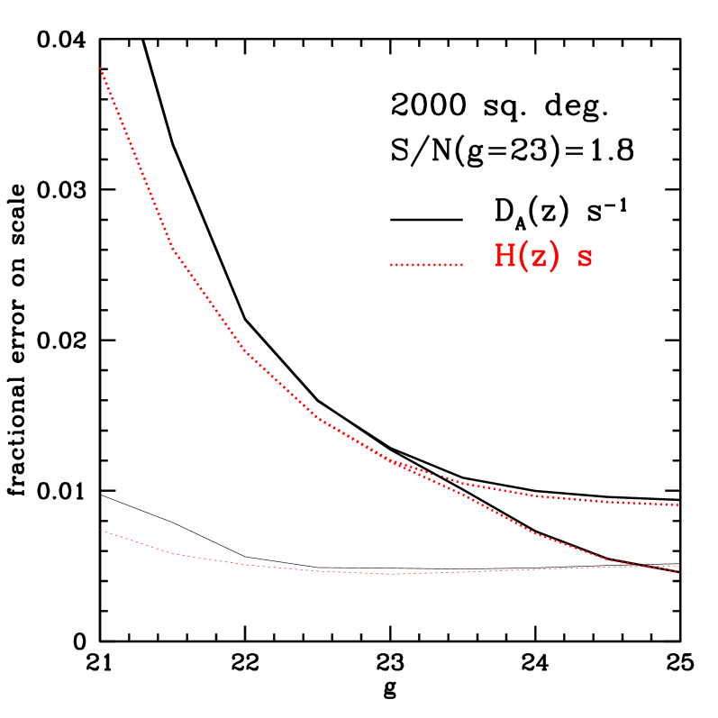
Figure 1: Upper thick lines show constraints as a function of g magnitude limit on the radial and transverse BAO scales for a survey similar to the proposed WFMOS low-z galaxy survey (Glazebrook et al., 2005), assuming 2000 sq. deg. and R=2000. Magnitude limits (21, 22, 23, 24, 25) correspond to (8, 20, 41, 77, 136) quasars per sq. deg. for the Jiang et al. (2006) luminosity function, and we assume S/N=(11, 4.5, 1.8, 0.7, 0.3) per Å. Lower thick curves add spectra from LBGs. Thin lines show the completely unrealistic case where we ignore the aliasing-like noise power caused by discrete sampling.

The WFMOS galaxy survey Glazebrook et al. (2005) is expected to obtain $1\sigma$ errors of 1.0 and 1.2% on $D_{A}(z)$ and $H(z)$, respectively, at $z\sim 1$, and, more relevantly, 1.5 and 1.8% at $z\sim 3$ from a separate, similarly costly, high z galaxy survey reaching $R<24.5$. Our errors depend on the magnitude limit, reaching better than 1.4% in both directions for $g<23$. The results improve more slowly with increasing magnitude limit because the faint spectra, at fixed observing time, are becoming too noisy to be very useful. If very faint quasars and LBGs can be identified, the errors could be as small as 0.5%. Note that the Ly$\alpha$ forest BAO measurement generally constrains $H(z)$ better than $D_{A}(z)$, the opposite trend from galaxies (Glazebrook et al., 2005).

To make the results clearer, we show the obtainable constraints on band power measurements in Fig. 2 (our standard constraints on the BAO scale do not go through this intermediate step).

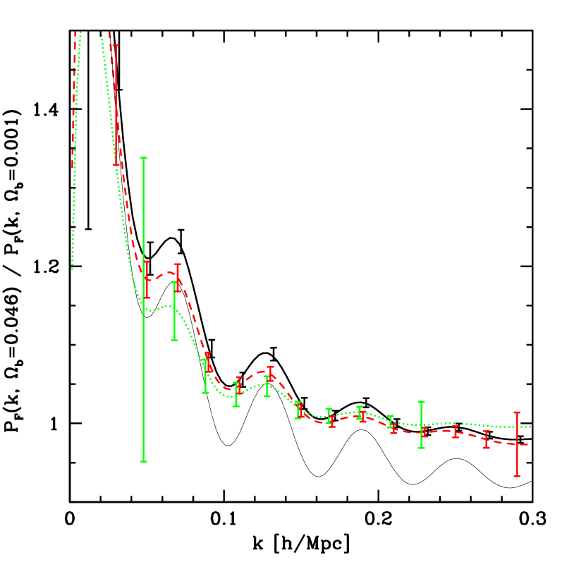
Figure 2: Error bars show the fractional error on the power in bands of $\Delta k=0.02\,h\,{\rm Mpc}^{-1}$, for the $g<25$ case from Fig. 1 (without LRGs). Lines show the ratio of Ly$\alpha$ forest flux power for $\Omega_{b}=0.0462$ to $\Omega_{b}=0.001$. Black (solid line, error bars shifted slightly right) shows $\mu=k_{\parallel}/k>2/3$, red (dashed) shows $1/3<\mu<2/3$, and green (dotted, error bars shifted left) shows $\mu<1/3$. For comparison, the thin line shows the ratio of power without aliasing noise (renormalized for clarity).

We see how the inclusion of aliasing-like power from the discrete transverse sampling, i.e., the 2nd term in Eq. (13), dilutes the amplitude of the BAO features, especially for modes transverse to the line of sight which are not enhanced by large-scale peculiar velocities. The absence of low-k transverse modes can be traced, somewhat counter-intuitively, to the fairly large minimum $k_{\parallel}$ resulting from the relatively small radial extent of the survey compounded by the loss of modes dropped to allow for continuum fitting. The absence of high k transverse modes is due to the sparse transverse sampling. Spectral noise power is, by construction, always subdominant ($\sim 50$% of the signal power including aliasing power), because quasars faint enough to contribute a lot of noise power are discarded by the weighting.

For comparison, in Fig. 3 we imagine piggy-backing the Ly$\alpha$ forest survey onto the high-z galaxy survey of Glazebrook et al. (2005), which is proposed to cover 300 sq. deg. with 240 minute exposures, obtaining errors of 1.8% on $H(z)$ and 1.5% on $D_{A}(z)$ using galaxies (note that the S/N we assume is guided by but should not be taken as a prediction for WFMOS sensitivity).

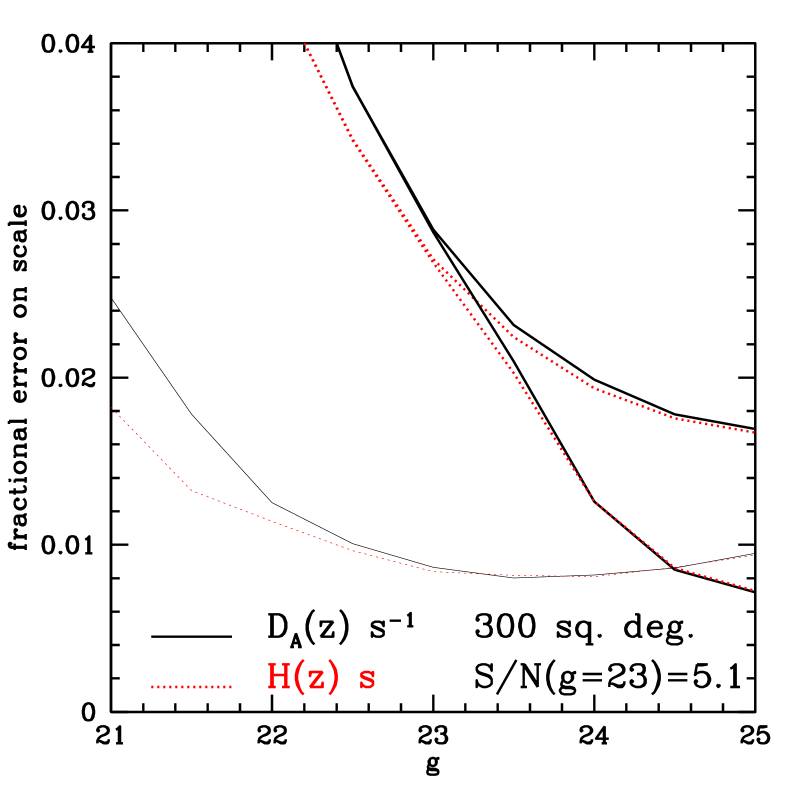
Figure 3: Similar to Fig. 1, except covering 300 sq. deg. with longer exposures, following the high-z galaxy survey proposed in Glazebrook et al. (2005). g magnitude limits (21, 22, 23, 24, 25) correspond to S/N=(32, 13, 5.1, 2.0, 0.8) per Å.

We find similar errors to those from galaxies at a similar limiting magnitude, but the wider, shallower survey is probably a better option for the Ly$\alpha$ forest. These figures uncover an important issue for survey planning: for a fixed survey configuration, the results are quite sensitive to the limiting magnitude, i.e., how bright does a quasar have to be to be identifiable?

We now explore the optimization of the survey. The errors scale precisely as $A^{-1/2}$ down to surveys much smaller than the ones we are discussing. It seems likely that any spectrograph used for this project will have more fibers than necessary, so the main question is how long to integrate before moving on to gather more area. Figure 4 shows the expected errors as a function of the S/N obtained per Å for a g=22.5 quasar, with a corresponding rescaling of the survey area to keep $A~{}(S/N)^{2}$ fixed.

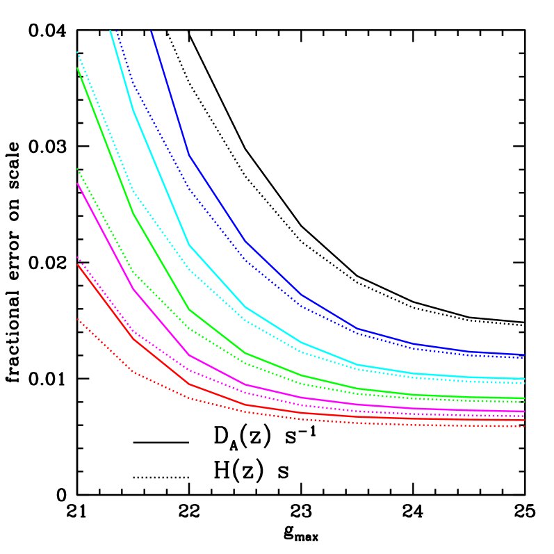
Figure 4: Similar to Fig. 1, but investigating the effect of the trade-off between noise and area. From top to bottom (black, blue, cyan, green, magenta, red) we show, at g=22.5, S/N=(5.7, 4.1, 2.9, 2.0, 1.4, 1.0) per Å. The results improve with decreasing S/N because in each case the area of the survey is $A=2000~{}(2.9~{}N/S)^{2}$ sq. deg., assuming sky-dominated noise. Errors scale as $A^{-1/2}$.

As in previous figures, we are including a realistic distribution of magnitudes, i.e., the noise is higher for fainter quasars and lower for brighter ones. We see that a wider, noisier survey is generally superior. Limitations on this progression will be set by telescope overhead and the minimum S/N needed to identify a quasar. We isolate the change with noise level in Fig. 5.

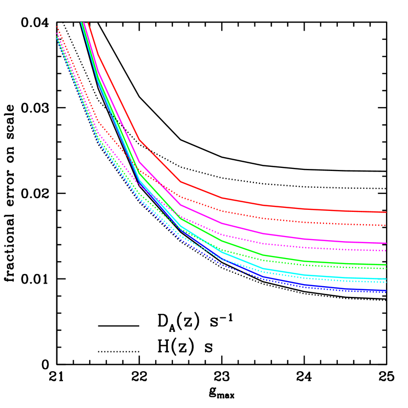
Figure 5: Similar to Fig. 1, but investigating the effect of the changing the noise level at fixed 2000 sq. deg. survey area. From bottom to top (black, blue, cyan, green, magenta, red, black) we show, at g=22.5, S/N=(5.7, 4.1, 2.9, 2.0, 1.4, 1.0, 0.72) per Å.

In Fig. 6, we show the effect of decreasing resolution.

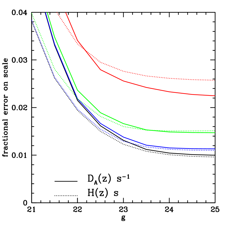
Figure 6: Similar to Fig. 1, but investigating the effect of changing resolution. From bottom to top (black, blue, green, red) lines show R=(2000, 250, 125, 62.5).

Only relatively poor resolution is needed. R=250 is essentially as good as 2000, and 125 is not too bad. These numbers are easy to understand. At R=125, the power suppression factor at our FKP weight point, $k=0.07\,h\,{\rm Mpc}^{-1}$, $\mu=0.5$, is only 11%. This suppression factor increases very quickly with $k_{\parallel}$; however, the aliasing noise that we show in Fig. 2 is itself suppressed by limited resolution, so the effect is somewhat less than one might otherwise expect.

Finally, we perform a few tests to make sure our calculation is robust. First, to test our code, we recompute the errors for the galaxy survey in Glazebrook et al. (2005). We can do this easily by dropping the aliasing term, setting the noise variance in cells defined by the pixel size and mean separation of the spectra to the inverse of the mean number of galaxies in a cell, and replacing the Ly$\alpha$ forest flux power spectrum with the galaxy power spectrum. We find errors 1.5% on $D_{A}(z)$ and 1.6% on $H(z)$, assuming they used $\Omega_{m}=0.35$, $\sigma_{8}=0.9$, $b=3.3$, $h=0.65$, $n=1.0$, following Seo and Eisenstein (2003). This compares well with Glazebrook et al. (2005)’s 1.5% and 1.8%, respectively.

One approximation we have made is to ignore evolution, i.e., to use the power spectrum, quasar number density, etc. from the center of the redshift interval for the full interval. As a test, we split the sample into two redshift bins, and compute the Fisher matrix separately for each, including marginalizing over two independent sets of nuisance parameters. The errors on each bin increase of course, but the combination of the two bins actually gives slightly smaller errors than the original full Fisher matrix, because of small differences in the averaging. Not surprisingly, the low redshift half of the survey gives significantly smaller error bars than the high redshift half (the quasar density is higher at fixed apparent magnitude at low $z$).

To test that we are really measuring the BAO feature and not some broadband feature in the power spectrum, we run our error computation using a transfer function with $\Omega_{b}=0.001$. We find that the errors for the survey in Fig. 1 are always greater than 5%, i.e., our measurement is clearly based on the baryonic feature. Finally, we note that our results are completely insensitive to removing the marginalization over $\beta$ or adding a marginalization over the noise amplitude.

A 30 sq. deg. pilot study reaching $g<21$ with $S/N=11$ at $g=21$ should detect baryon oscillations at $\sim 2\sigma$, in the sense that the Fisher matrix prediction for a measurement of $\Omega_{b}$, marginalized over the nuisance parameters discussed above, predicts an error 0.023 for $\Omega_{b}=0.046$. Reaching $g<22$ with $S/N>4.5$ would produce a $2.7\sigma$ detection. A detection of this kind would not be fundamentally interesting; rather, we give these numbers to indicate the type of survey that would be needed to produce a good solid measurement of the Ly$\alpha$ forest power on the appropriate scale. As usual, a survey four times larger with half this $S/N$ would produce a better measurement.

IV Constraints on Dark Energy and Curvature

In §IV.1, we give projected constraints on the most standard specific parameterization of the dark energy. In §IV.2 we discuss the general usefulness of a BAO measurement at $z>2$, in a non-parametric way.

IV.1 Parametric models

We discuss first the usefulness of a BAO measurement at $z\sim 2.8$ for constraining dark energy with equation of state $w(a)=w_{0.6}+(0.6-a)~{}w^{\prime}$, with $w_{0.6}$ and $w^{\prime}$ as parameters. We saw above that the true center of weight of the Ly$\alpha$ forest survey would probably be a bit lower than $z\sim 2.8$ but we find negligible sensitivity of the final constraints to the exact Ly$\alpha$ forest redshift. The pivot point $a=0.6$ was chosen to make $w_{a}$ and $w^{\prime}$ roughly uncorrelated for our scenarios. We use the figure of merit (FoM) defined by the Dark Energy Task Force (DETF) as our primary measure of survey value. The DETF FoM is simply the inverse of the area within the 95% confidence contour in the $w_{a}-w^{\prime}$ plane, which has the important characteristic of being independent of the chosen pivot point.

We include the projected constraints from the Planck CMB experiment. We use standard Fisher matrix techniques (Eisenstein et al., 1999; Hu, 2002), following Bond et al. (2004) in ignoring foregrounds but using only the 143 GHz channel. Our results agree well with Bond et al. (2004) when we use similar parameter combinations. For reproducibility, our results are given in Table 1.

Table 1: Assumed values, errors, and error correlations from Planck. The first row is the assumed value of the parameter, the second is the error, and the rest are the correlation matrix. Very large errors should be interpreted only qualitatively.

	$n_{s}$	$w_{0.6}$	$\Omega_{k}$	$\omega_{b}$	$\omega_{m}$	$\theta_{s}$	$\tau$	$\log_{10}(A)$	$w^{\prime}$
$p$	0.963	-1.00	0.00	0.0227	0.145	0.597	0.0994	-8.65	0.00
$\sigma$	0.0043	0.22	0.021	0.00017	0.0015	0.00032	0.0046	0.0038	4.1
$n_{s}$	1.000	-0.078	0.034	0.594	-0.842	0.294	0.320	-0.075	-0.119
$w_{0.6}$	-0.078	1.000	0.577	0.058	-0.004	-0.104	0.034	0.045	-0.006
$\Omega_{k}$	0.034	0.577	1.000	0.161	-0.117	0.192	0.180	0.146	0.315
$\omega_{b}$	0.594	0.058	0.161	1.000	-0.645	0.352	0.252	0.000	-0.019
$\omega_{m}$	-0.842	-0.004	-0.117	-0.645	1.000	-0.282	-0.308	0.110	0.069
$\theta_{s}$	0.294	-0.104	0.192	0.352	-0.282	1.000	0.079	-0.010	0.684
$\tau$	0.320	0.034	0.180	0.252	-0.308	0.079	1.000	0.899	-0.059
$\log_{10}(A)$	-0.075	0.045	0.146	0.000	0.110	-0.010	0.899	1.000	-0.018
$w^{\prime}$	-0.119	-0.006	0.315	-0.019	0.069	0.684	-0.059	-0.018	1.000

We see that the CMB alone only weakly constrains dark energy (note here that the Fisher matrix technique may not give reliable errors in cases where the errors are large, but this should not be a problem once other data constrains these degenerate directions).

Table 2 shows the FoM and constraints on $w_{0.6}$, $w^{\prime}$, and sometimes $\Omega_{k}$, for several different combinations of data.

Table 2: Errors on $w_{0.6}$, $w^{\prime}$, and $\Omega_{k}$ [with $w(a)=w_{0.6}+(0.6-a)~{}w^{\prime}$] for different data combinations, along with the DETF figure of merit (FoM), defined to be the inverse area inside the $2-\sigma$ contours in the $w_{0.6}-w^{\prime}$ plane. BAO errors are 5.8% radial and 5.2% transverse at $z=0.3$, and 1% in both directions at $z=2.8$. The $z\sim 1$ constraint is a set of points in the range $0.6<z<1.2$, with combined precision equal to the $z=2.8$ constraint (see text).

	BAO	BAO	BAO
Planck	$z=0.3$	$z\sim 1$	$z=2.8$	FoM	$\sigma_{w_{0.6}}$	$\sigma_{w^{\prime}}$	$\sigma_{\Omega_{k}}$
Y	Y	N	N	0.16	0.211	2.37	0.0100
Y	Y	Y	N	0.75	0.091	1.48	0.0038
Y	Y	N	Y	0.52	0.127	1.36	0.0031
Y	Y	Y	Y	1.40	0.068	0.84	0.0022
Y	Y	N	N	0.27	0.130	2.30	—
Y	Y	Y	N	1.31	0.074	0.87	—
Y	Y	N	Y	0.54	0.122	1.35	—
Y	Y	Y	Y	1.61	0.067	0.74	—

To avoid sensitivity to broad-band power, we use separate (independent) slope and amplitude parameters for the CMB and Ly$\alpha$ forest. We use three different BAO constraints: First, we always assume that SDSS will produce a 5.8% error on the radial scale at $z=0.3$, $v_{s}(z=0.3)$, and 5.2% error on the transverse scale, $\theta_{s}(z=0.3)$ (Seo and Eisenstein, 2003). We optionally add a 1% constraint on both distance scales at $z=2.8$. Finally, we optionally include a $\sim 1$% constraint at $z\sim 1$. To avoid artificially degrading the value of a $z\sim 1$ survey, we spread this measurement over points at $z=0.6,0.8,1.0$, and 1.2, using the relative errors from Seo and Eisenstein (2003) but modifying the overall normalization to make the combined error from the eight points $0.7$%, i.e., the same total precision as the two 1% $z=2.8$ measurements. We choose a simple 1% because different survey configurations can lead to many different combinations of errors. The point here is primarily to study the general usefulness of constraints at different redshifts, not any specific survey.

We see, as expected, that in the presence of Planck constraints the measurement at $z=2.8$ is less valuable for constraining dark energy than the measurement at $z\sim 1$; however, if $\Omega_{k}$ is allowed to vary, adding the $z=2.8$ measurement nearly doubles the DETF FoM. This improvement is larger than the affect of doubling the size of the $z\sim 1$ survey. The higher $z$ measurement is actually slightly more valuable than $z\sim 1$ for constraining $\Omega_{k}$. If we assume flatness the improvement is more modest, although not completely negligible. If the CMB is taken out of play for some reason, the $z=2.8$ measurement becomes more valuable than $z=1$, although in that case both are really needed to provide an interesting measurement.

We note that the commonly used approximation that the Planck constraint can be represented by the constraints on $\theta_{s}$ (0.04%, or perfectly known) and $\omega_{m}$ (1%) alone, treated as independent of each other and other parameters, works very well, in the sense that the resulting FoM agrees with the full-Fisher matrix version to better than 10%.

IV.2 Non-parametric

We will next consider the measurement of the acoustic scale at $z\gtrsim 2$ in the context of testing the flat $\Lambda$CDM model. We will expand in small perturbations around the fiducial model, working to lowest order in the non-constant dark energy and curvature. Hence, we write $H^{2}=(8\pi G/3)(\rho_{\rm fid}+\rho_{X})+\Omega_{K}H_{0}^{2}(1+z)^{2}$, where $\rho_{\rm fid}$ is the sum of the matter, radiation, and cosmological constant contributions and $\rho_{X}$ includes the dark energy density that differs from the $z=0$ value. We want to test whether $\rho_{X}=0$ or not, keeping in mind the uncertainties in $\rho_{\rm fid}$ and curvature.

IV.2.1 Transverse Scale

In the transverse direction, we measure $\ell_{z}=\theta_{s}(z)^{-1}=(1+z)D_{A}(z)/s$. For example, we measure $\ell_{1089}$ to wonderful accuracy (0.35% with 3-year WMAP, $\ll 0.1\%$ with Planck). Now we consider a measurement at $z\approx 2$ and construct $\ell_{1089}-\ell_{z}$ as a way to isolate the new information beyond that available in the CMB. To lowest order in curvature, the angular diameter distance

$$(1+z)D_{A}=r+\frac{\Omega_{K}}{6}\frac{H_{0}^{2}r^{3}}{c^{2}}.$$ (20)

This then yields

$$\ell_{1089}-\ell_{z} = \frac{1090D_{A}(1089)-(1+z)D_{A}(z)}{s}\approx\frac{r(1089)-r(z)}{s}+\frac{\Omega_{K}H_{0}^{2}}{6sc^{2}}\left[r^{3}(1089)-r^{3}(z)\right]$$ (21)

$$= \frac{1}{s}\int_{z}^{1089}\frac{c\;dz}{H}+\frac{\Omega_{K}H_{0}^{2}}{6sc^{2}}\left[r^{2}(1089)+r(1089)r(z)+r^{2}(z)\right]\int_{z}^{1089}\frac{c\;dz}{H_{\rm fid}}$$

$$\approx \frac{1}{s}\left[1+\frac{\Omega_{K}}{6}\frac{H_{0}^{2}r^{2}(1089)}{c^{2}}\left(1+d+d^{2}\right)\right]\int_{z}^{1089}\frac{c\;dz}{H_{\rm fid}}-\frac{1}{2s}\int_{z}^{1089}\frac{c\;dz}{H_{\rm fid}}\left(\frac{\rho_{X}}{\rho_{\rm fid}}+\frac{3\Omega_{K}H_{0}^{2}(1+z)^{2}}{8\pi G\rho_{\rm fid}}\right)$$

where we’ve define $d=r(z)/r(1089)$ and assumed that $|\Omega_{K}|\ll 1$ and $\rho_{X}\ll\rho_{\rm fid}$ (suitable for $z\gtrsim 2$). The latter means that $\rho_{X}/\rho_{\rm fid}=\Omega_{X}$. Keeping only lowest order in the perturbations around the fiducial model, we also have

$$\frac{3\Omega_{K}H_{0}^{2}(1+z)^{2}}{8\pi G\rho_{\rm fid}}=\frac{\Omega_{K}(1+z)^{2}}{\Omega_{m}(1+z)^{3}+\Omega_{\Lambda}}\approx\frac{\Omega_{K}}{\Omega_{m}(1+z)}\left[1-2\lambda+O(\lambda^{2})\right]$$ (22)

where $\lambda=\Omega_{\Lambda}/2\Omega_{m}(1+z)^{3}$. We can drop the higher orders in $\lambda$ when working at higher redshift.

We now define a weighted average of $\Omega_{X}$

$$\bar{\Omega}_{X}\equiv\frac{\int_{z}^{1089}\frac{c\;dz}{H_{\rm fid}}\Omega_{X}}{\int_{z}^{1089}\frac{c\;dz}{H_{\rm fid}}}$$ (23)

and rearrange to find

$$\bar{\Omega}_{X}=2+\frac{2s}{\int_{z}^{1089}\frac{c\;dz}{H_{\rm fid}}}\left(\ell_{z}-\ell_{1089}\right)+\Omega_{K}\left[\frac{H_{0}}{3c^{2}}r^{2}(1089)(1+d+d^{2})-\frac{1-\frac{6\lambda}{7}}{3\Omega_{m}(1+z)}\right].$$ (24)

The last term comes from doing the integral for the curvature term in (21). For standard cosmologies, the coefficient in square brackets is about 5 for $z=2$-3. The middle term must be $-2$ in the fiducial model, because the result cancels to $\bar{\Omega}_{X}=0$.

The question is now how accurately we can measure $\bar{\Omega}_{X}$ in light of the uncertainties on the various terms on the right-hand side of the equation. In particular, we want to know how the uncertainties in $\Omega_{m}h^{2}$, $\Omega_{m}$, and $\Omega_{\Lambda}$ enter (i.e., how well specified the baseline model is). It is useful to rearrange the middle term as

$$2\left[s(\Omega_{m}H_{0}^{2})^{1/4}\right](\Omega_{m}H_{0}^{2})^{1/4}\left[\sqrt{\Omega_{m}H_{0}^{2}}\int_{z}^{1089}\frac{c\;dz}{H_{\rm fid}}\right]^{-1}\left(\ell_{z}-\ell_{1089}\right)$$ (25)

The combination $s(\Omega_{m}H_{0}^{2})^{1/4}$ is picked to cancel out most of the dependence of $s$ on $\Omega_{m}H_{0}^{2}$. We can manipulate the integral as

$$\int_{z}^{1089}\frac{c\;dz}{H_{\rm fid}}=\frac{c}{\sqrt{\Omega_{m}H_{0}^{2}}}\int_{z}^{1089}\frac{dz}{\sqrt{(1+z)^{3}+(\Omega_{r}/\Omega_{m})(1+z)^{4}}}\left[1+\frac{\Omega_{\Lambda}}{\Omega_{m}}(1+z)^{-3}\right]^{-1/2}~{}.$$ (26)

If we expand the square bracket terms and neglect the radiation term when integrating the terms with $\Lambda$, then we find

$$\int_{z}^{1089}\frac{c\;dz}{H_{\rm fid}}=\frac{c}{\sqrt{\Omega_{m}H_{0}^{2}}}\left[\int_{z}^{1089}\frac{dz}{\sqrt{(1+z)^{3}+(\Omega_{r}/\Omega_{m})(1+z)^{4}}}-\frac{2}{\sqrt{1+z}}\left(\frac{\lambda}{7}-\frac{3\lambda^{2}}{26}+\ldots\right)\right]$$ (27)

$$=\frac{2c}{\sqrt{\Omega_{m}H_{0}^{2}}}\left[\left.\sqrt{a+a_{eq}}\right|^{z}_{1089}-\frac{1}{\sqrt{1+z}}\left(\frac{\lambda}{7}-\frac{3\lambda^{2}}{26}+\ldots\right)\right]$$ (28)

where $a=1/(1+z)$. With this, we find

$$\bar{\Omega}_{X} = 2+\frac{\sqrt{1+z}}{c}\left[s(\Omega_{m}H_{0}^{2})^{1/4}\right](\Omega_{m}H_{0}^{2})^{1/4}\left(\ell_{z}-\ell_{1089}\right)\left[1-\sqrt{(1+z)\left(\frac{1}{1090}+\frac{1}{z_{eq}}\right)}-\frac{\lambda}{7}+\frac{3\lambda^{2}}{26}+O(\lambda^{3})\right]^{-1}$$ (29)

$$+\Omega_{K}\left[\frac{H_{0}}{3c^{2}}r^{2}(1089)(1+d+d^{2})-\frac{1-\frac{6\lambda}{7}+O(\lambda^{2})}{\Omega_{m}(1+z)}\right].$$

Now we can look at the errors in these terms. We denote $\sigma(x)$ as the standard deviation of $x$. The error in $\Omega_{m}h^{2}$ is expected to be below 2% with Planck data. That means that the fractional error in $(\Omega_{m}H_{0}^{2})^{1/4}$ is below 0.5%. The quantity $s(\Omega_{m}H^{2})^{1/4}$ essentially depends only on $\Omega_{b}h^{2}$, but this is to the $1/8$ power, so the error will be below 0.1%. For $\lambda$,

$$\sigma(\lambda)=\frac{1}{2(1+z)^{3}\Omega_{m}}\frac{\sigma(\Omega_{m})}{\Omega_{m}}.$$ (30)

As we care about $\lambda/7$, the value ends up being about $\sigma(\lambda/7)=\sigma(\Omega_{m})(1+z)^{-3}$. With today’s cosmological constraints (e.g., Eisenstein et al. (2005); Seljak et al. (2006)), this error is about 0.1% at $z=2$; of course, this will shrink in the future. In other words, our low redshift data constrains $\Lambda$ well enough that the uncertainties in the extrapolation to $z>2$ are tiny. The contribution of $\lambda$ in the curvature term is smaller yet; we will drop these. The errors in the radiation term $z_{eq}$ are very small.

This leaves the fractional error in $\ell_{z}-\ell_{1089}$. The error in $\ell_{1089}$ will be very small with Planck, so we neglect it. Then

$$\frac{\sigma(\ell_{z}-\ell_{1089})}{\ell_{z}-\ell_{1089}}=\frac{\sigma(\ell_{z})}{\ell_{z}}\frac{1}{\ell_{1089}/\ell_{z}-1}$$ (31)

The quantity $\ell_{1089}/\ell_{z}-1$ is 1.7 for $z=2$ and 1.2 for $z=3$.

Hence, the error in $\bar{\Omega}_{X}$ is dominated by the quadrature sum of half the fractional error in $\Omega_{m}h^{2}$ ($\lesssim 1\%$ for Planck), the fractional error in $\ell_{z}$ times $2/(\ell_{1089}/\ell_{z}-1)$ (which is 1–1.7, depending on redshift), and five times the uncertainty in the curvature $\Omega_{K}$. Of course, one might opt to move the curvature to the other side of the ledger and constrain $\bar{\Omega}_{X}-5\Omega_{K}$.

It is a good approximation to think of $\bar{\Omega}_{X}$ as

$$\bar{\Omega}_{X}\approx\frac{\int_{a_{eq}}^{a}d\ln a\;a^{1/2}\Omega_{X}}{\int_{a_{eq}}^{a}d\ln a\;a^{1/2}}$$ (32)

One might compare this to the effect of anomalous dark energy on the growth of structure, which enters as a suppression of growth approximately as a factor

$$1-\frac{3}{5}\int_{a_{eq}}^{a}d\ln a\;\Omega_{X}$$ (33)

The weightings differ by $a^{1/2}$.

IV.2.2 Radial Scale

Next, we turn to the radial acoustic scale. Here we are measuring $v_{s}(z)=sH(z)/(1+z)$ at a given $z$. Performing the same expansion, we have

$$v_{s}(z)=s\frac{H_{\rm fid}(z)}{1+z}\left(1+\frac{\rho_{X}}{2\rho_{\rm fid}}+\frac{3\Omega_{K}H_{0}^{2}(1+z)^{2}}{8\pi G\rho_{\rm fid}}\right)=s~{}(1+z)^{1/2}\sqrt{\Omega_{m}H_{0}^{2}}\left[1+\frac{\Omega_{\Lambda}}{\Omega_{m}(1+z)^{3}}\right]^{1/2}\left(1+\frac{\Omega_{X}}{2}+\frac{1}{2}\frac{3\Omega_{K}H_{0}^{2}(1+z)^{2}}{8\pi G\rho_{\rm fid}}\right)$$ (34)

If we expand in powers of $\lambda$, we get

$$v_{s}(z)=\left[s(\Omega_{m}H_{0}^{2})^{1/4}\right](1+z)^{1/2}(\Omega_{m}H_{0}^{2})^{1/4}\left[1+\lambda-\frac{\lambda^{2}}{2}+O(\lambda^{3})\right]\left[1+\frac{\Omega_{X}}{2}+\frac{\Omega_{K}}{2\Omega_{m}(1+z)}(1-2\lambda+O(\lambda^{2}))\right]$$ (35)

Solving for $\Omega_{X}$, we have

$$\Omega_{X}=-2+2~{}v_{s}(z)~{}(1+z)^{-1/2}\left[s(\Omega_{m}H_{0}^{2})^{1/4}\right]^{-1}(\Omega_{m}H_{0}^{2})^{-1/4}\left[1+\lambda-\frac{\lambda^{2}}{2}+O(\lambda^{3})\right]^{-1}-\frac{\Omega_{K}}{\Omega_{m}(1+z)}(1-2\lambda+O(\lambda^{2}))$$ (36)

Again, the middle term must be $2$ in the fiducial model.

Looking at the error budget, again we expect to know $(\Omega_{m}H_{0}^{2})^{1/4}$ to better than 0.5%. The error in $\lambda$ is about $\sigma(\Omega_{m})/4$ at $z=2$, which is already about 0.7% today and should drop toward 0.1%. The coefficient of $\Omega_{K}$ will be about unity for a survey at $z\approx 3$. So the error in $\Omega_{X}$ is about the quadrature sum of half the fractional error in $\Omega_{m}H_{0}^{2}$ (somewhat below 1%), twice the fractional error in the acoustic scale $v_{s}(z)$, and the error on $\Omega_{K}$.

IV.2.3 Measurement Goals

It is not clear what quantitative goal one wants to set for the measurement of $\Omega_{X}$ or $\bar{\Omega}_{X}$. One goal is to simply detect the cosmological constant at high redshift, i.e., to exclude $\Omega_{X}(z)=-\Omega_{\Lambda}(z)$. When one averages this model over redshift, one gets $\bar{\Omega}_{X}=\Omega_{\Lambda}/7\Omega_{m}(1+z)^{3}$. This is only about 1% at $z=2$. Hence, it is very hard to detect the absence of high-redshift dark energy using the transverse distance scale. However, it is fairly easy with the radial scale: $\Omega_{X}=-\Omega_{\Lambda}/\Omega_{m}(1+z)^{3}$ is about 10% at $z=2$ and 4% at $z=3$. A 1% measurement of $H(z)$ at $z=2$ should detect the dark energy at 3 to 5 $\sigma$, depending on whether the error bars on $\Omega_{m}h^{2}$ are 2% or somewhat better.

Of course, extra dark energy can be detected too. The 1% measurement of $H(z)$ would bound (at 3-5 $\sigma$) the energy density of the dark energy at $z=2$ to be within a factor of two of its low redshift value.

The above statements assumes a flat cosmology, but the sensitivity of the transverse scale to curvature is 5 times larger than that of the radial scale. Hence, one can use the transverse acoustic scale to control the curvature to levels well smaller than the errors on the $\Omega_{X}$ measurement from the radial acoustic scale; this assumes that $\bar{\Omega}_{X}\lesssim\Omega_{X}$. Putting this another way, one can mix the transverse and radial scale to produce a curvature-independent measurement of a combination $\Omega_{X}+\bar{\Omega}_{X}/5$, the coefficient being appropriate to the redshifts considered here, Many dark energy models will not yield zero for this combination; this would require that $\Omega_{X}$ is larger at redshifts above the survey redshift and of the opposite sign. Hence, one can perform a reasonably generic search for deviations from the cosmological constant at the survey redshift.

Whether this is interesting depends considerably on one’s model for dark energy. The $w=w_{0}+w_{a}(1-a)$ model has the unfortunate property of demanding that there are no changes in dark energy at high redshift that aren’t heralded with even larger changes at low redshifts. If one relaxes that assumption it is certainly the case that we don’t know the dark energy density at $z=2$ to 30% rms.

Another question is whether there is a steady value of $\Omega_{X}$ at high redshift, as tracker models would have Zlatev et al. (1999). Here, $\bar{\Omega}_{X}$ is reasonably close to $\Omega_{X}$, and one could reach a error bar of about 1%, assuming a flat cosmology. One may compare this to constraint available from measuring the growth of structure relative to the CMB. Here, one is limited by the optical depth to $z=1000$. With Planck, this may be measured as well as 0.5%, so if one could measure the growth function to that level, one could measure a value of $\Omega_{X}$ in the 0.1-0.2% range (1-$\sigma$). This method, however, is at least partially degenerate with the suppression caused by non-zero neutrino mass Hu et al. (1998). A suppression of 0.5% corresponds to about 0.015 eV, already well into the region indicated by the atmospheric neutrino results. Hence, the degeneracy between neutrino mass will be an issue as one tries to push constraints on $\Omega_{X}$ below 1%.

Looking beyond the scope of the surveys discussed in this paper, the full-sky cosmic variance limit on the acoustic scale at these redshifts is superb. At this point, the uncertainty on $\Omega_{m}h^{2}$ from CMB experiments such as Planck will produce sufficient uncertainty in the acoustic scale as to dominate the error budget on $\Omega_{X}$ or $\bar{\Omega}_{X}$. From a statistical point of view, such BAO surveys themselves could measure $\Omega_{m}h^{2}$ better than the CMB, thereby restoring the precision in the sound horizon, but the systematics in broad-band power measurement from low-redshift surveys will surely be worse than those in the CMB. Another option is to form a combination $\Omega_{X}+\bar{\Omega}_{X}$ that is independent of $\Omega_{m}h^{2}$. This combination, however, is not independent of curvature; essentially one is using the angular acoustic scale in the CMB to calibrate $\Omega_{m}h^{2}$. Nevertheless, this is a simple example of the idea that the BAO measurement of $D_{A}(z)$ and $H(z)$ does produce an internal cross-check, namely that $D_{A}$ is an integral of $H(z)$, that can be used to eliminate certain nuisance parameters.

V Conclusions

As a probe of dark energy, baryonic acoustic oscillation features have a significant advantage over standard candles such as supernovas in that we have a very clear theory describing them. Even the imperfection associated with our lack of understanding of exactly how galaxies populate dark matter halos does not present a significant problem, because the scale of halos is well separated from the scale of the BAO. The Ly$\alpha$ forest extends this advantage in that we can perform something relatively close to a computation from first-principles.

In this paper we have computed the statistical power that can be expected from a large, three-dimensional Ly$\alpha$ forest survey probing the BAO scale. If the Universe is not assumed to be flat, a measurement of the BAO scale at $z\sim 3$ provides a interestingly large improvement in the constraints on dark energy, as quantified in §IV using the Dark Energy Task Force figure of merit. A range of combinations of area and magnitude limit could lead to a viable survey, as described in §III. Resolution and signal-to-noise ratio requirements are modest. It will probably be most efficient to piggy-back Ly$\alpha$ forest surveys on top of lower redshift galaxy surveys.

As with other probes, the Ly$\alpha$ forest version of the BAO measurement should be robust against systematic errors. Long-range effects in the UV ionizing background will not produce preferred scales and can’t mimic the acoustic peak. The poorly modeled highest density absorption (e.g., DLAs) will not produce a BAO signal either. Continuum features could possibly create a bump on the appropriate scale, but these should be easy to control because they would be associated with fixed quasar rest wavelength ranges, unlike the BAO feature. In the worst case we would lose only a small fraction of pixel-pairs by completely ignoring correlation between pixels in the same spectrum. Since we would be using multiobject spectrograph techniques, fluxing errors would create density variations as a function of redshift for all objects in a region. This creates fake large-scale power; however, one can project this purely radial power out with minimal information loss (Seljak, 1998; Tegmark et al., 1998).

The ultimate Ly$\alpha$ forest survey could include faint Lyman break galaxies to obtain a higher density of probes. However, getting a redshift for these galaxies is not trivial. For the 75% that don’t have Lya emission, one needs to integrate down to the continuum, which will require higher S/N than to obtain the redshift of a quasar QSO. At this point we also know less about possible relevant variations in galaxy continua.

In the short term, a pilot study aimed at simply detecting the BAO feature in the Ly$\alpha$ forest would be very desirable. The bare minimum requirements are roughly $>30$ square degrees with a magnitude limit $g>21$.