Annual Modulation of Dark Matter in the Presence of Streams

Abstract

In addition to a smooth component of WIMP dark matter in galaxies, there may be streams of material; the effects of WIMP streams on direct detection experiments is examined in this paper. The contribution to the count rate due to the stream cuts off at some characteristic energy. Near this cutoff energy, the stream contribution to the annual modulation of recoils in the detector is comparable to that of the thermalized halo, even if the stream represents only a small portion ($\sim$5% or less) of the local halo density. Consequently the total modulation may be quite different than would be expected for the standard halo model alone: it may not be cosine-like and can peak at a different date than expected. The effects of speed, direction, density, and velocity dispersion of a stream on the modulation are examined. We describe how the observation of a modulation can be used to determine these stream parameters. Alternatively, the presence of a dropoff in the recoil spectrum can be used to determine the WIMP mass if the stream speed is known. The annual modulation of the cutoff energy together with the annual modulation of the overall signal provide a “smoking gun” for WIMP detection.

I Introduction

The Milky Way, along with other galaxies, is well known to be encompassed in a massive dark matter halo of unknown composition. Leading candidates for this dark matter are Weakly Interacting Massive Particles (WIMPs), a generic class of particles that includes the lightest supersymmetric particle. Numerous collaborations worldwide have been searching for these particles. Direct detection experiments attempt to observe the nuclear recoil caused by these dark matter particles interacting with nuclei in the detectors. These experiments include DAMA/NaI Bernabei:2003za , DAMA/LIBRA Bernabei:2005ki , NAIAD Alner:2005kt , CDMS Akerib:2005kh , EDELWEISS Sanglard:2005we , ZEPLIN Alner:2005pa , XENON Aprile:2004ey , DRIFT Alner:2004cw ; Alner:2005 , CRESST Angloher:2002in ; Angloher:2004tr , SIMPLE Girard:2005pt , PICASSO Barnabe-Heider:2003cq , COUPP Bolte:2005fm , and many others. It is well known that the count rate in WIMP direct detection experiments will experience an annual modulation Drukier:1986tm ; Freese:1987wu as a result of the motion of the Earth around the Sun: the relative velocity of the detector with respect to the WIMPs depends on the time of year.

The actual signals in a dark matter detector, including the modulation, depend on the distribution of WIMPs in the galaxy. It is commonly believed that a majority of the WIMPs have become thermalized into a smooth halo distribution. In the simplest model, the halo is a spherically symmetric, non-rotating isothermal sphere of WIMPs Freese:1987wu . The annual modulation of non-standard halos, such as anisotropic models, is discussed in Refs. Green:2000jg ; Green:2003yh ; Ullio:2000bf ; Fornengo:2003fm ; Copi:2002hm .

However, galaxy formation is a continual process, with new material still being accreted through, e.g., absorption of dwarf galaxies such as the Sagittarius dwarf galaxy Yanny:2003zu ; Newberg:2003cu ; Majewski:2003ux . The result is that the halo can contain a non-trivial amount of substructure such as clumps and tidal streams of material. The presence of such substructure is supported by $N$-body simulations of galaxy formation (see, e.g., Refs. Klypin:1999uc ; Moore:1999nt ). Unlike the virialized component of the halo, a clump or stream of material would result in a “cold” flow of WIMPs through a detector: the velocity dispersion is small relative to the typical speed with respect to the Earth, so that the WIMPs are incident from nearly the same direction and with nearly the same speed. Alternative models of halo formation, such as the late-infall model Gunn:1972sv ; Fillmore:1984wk ; Bertschinger:1900nj (more recently examined by Sikivie and others Sikivie:1992bk ; Sikivie:1996nn ; Sikivie:1997ng ; Sikivie:1999jv ; Tremaine:1998nk ; Natarajan:2005fh ), also predict cold flows of dark matter. Any such streaming of WIMPs (we will henceforth use “stream” to imply any cold flow) will yield a significantly different modulation effect than that due to a smooth halo. A stream actually provides two types of modulation: a modulation in the overall signal and a modulation in some cutoff energy above which counts due to the stream are not observed. Together, these two types of modulation can yield a “smoking gun” for WIMPs. The modulation in the presence of one or more streams is discussed in Refs. Gelmini:2000dm ; Stiff:2001dq ; Ling:2004aj ; Freese:2003na ; Freese:2003tt .

Here, we examine how various parameters describing a stream affect the modulation signal; the parameters examined are the stream direction, speed, density, and dispersion. We expect the stream density (and hence contribution to the recoil rate) to be small, $\mathcal{O}(\textrm{few\%})$ that of the isothermal Halo, and yet find that the stream can have significant effects on the annual modulation. We note the following interesting modifications to the overall annual modulation when we add the effects of the stream into the isothermal halo:

• The combined modulation generally does not have a cosinuoidal variation with time, even if the modulation of each individual component does;

• The combined modulation need not be time-symmetric, even if each individual components is; and

• The minimum and maximum recoil rates need not occur 0.5 years apart.

• Near the cutoff energy of the stream (above which it no longer contributes), the stream contribution to the annual modulation is comparable to that of the halo, even for a 2% stream density (relative to the background halo). The drastic effects of the stream near the cutoff energy can be seen in Figure 1 (for the modulation shown at 39 keV).

• The annual modulation of the cutoff energy together with the annual modulation of the overall signal provide a “smoking gun” for WIMP detection.

As a consequence of the second-to-last point, it is likely that the existence of a stream will be identified near its cutoff energy. Since a stream’s effects are mild except near $E_{c}$ (and essentially non-existent well above $E_{c}$), the presence of a stream should not interfere with using the modulation to describe the background distribution, SHM or otherwise.

In Section II, we will begin by reviewing direct detection techniques for WIMPs and the time-dependent WIMP recoil rate in an experimental detector. We will describe the Standard Halo Model (SHM) and examine the behavior of the modulation signals in this model in Section III. We will then examine how a dark matter stream affects this signal, first with the Sagittarius (Sgr) stream (Section IV), then generalizing to other streams (Section V). In Section V, we also briefly outline how various stream parameters can be extracted from a modulation signal. Our results are summarized in Section VI.

II Dark Matter Detection

WIMP direct detection experiments seek to measure the energy deposited when a WIMP interacts with a nucleus in the detector Goodman:1984dc . If a WIMP of mass $m$ scatters elastically from a nucleus of mass $M$, it will deposit a recoil energy $E=(\mu^{2}v^{2}/M)(1-\cos\theta)$, where $\mu\equiv mM/(m+M)$ is the reduced mass, $v$ is the speed of the WIMP relative to the nucleus, and $\theta$ is the scattering angle in the center of mass frame. The differential recoil rate per unit detector mass for a WIMP mass $m$, typically given in units of counts/kg/day/keV, can be written as:

$$\mathcal{R}\equiv\frac{\mathrm{d}R}{\mathrm{d}E}=\frac{\sigma(q)}{2m\mu^{2}}\,\rho\,\eta(E,t)$$ (1)

where $q=\sqrt{2ME}$ is the nucleus recoil momentum, $\sigma(q)$ is the WIMP-nucleus cross-section, $\rho$ is the local WIMP density, and information about the WIMP velocity distribution is encoded into the mean inverse speed $\eta(E,t)$,

$$\eta(E,t)=\int_{u>v_{\textrm{min}}}\frac{f(\mathbf{u},t)}{u}\,\mathrm{d}^{3}u\,.$$ (2)

Here

$$v_{\textrm{min}}=\sqrt{\frac{ME}{2\mu^{2}}}$$ (3)

represents the minimum WIMP velocity that can result in a recoil energy $E$ and $f({\bf u},t)$ is the (time-dependent) distribution of WIMP velocities ${\bf u}$ relative to the detector. For distinguishable WIMP populations (such as multiple streams), $\rho\eta\to\sum_{i}\rho_{i}\eta_{i}$ in Eqn. (1), where $\rho_{i}$ and $\eta_{i}$ are the local density and mean inverse speed, respectively, of some WIMP population indexed by $i$.

In this paper, the use of the term “rate” will refer to the differential rate $\mathcal{R}$. Dates will be given as fractions of a calendar year (i.e. from January 1). For example, June 1 will be given as $t=0.415$ years. For illustrative purposes, we will take $\sigma_{p}=10^{-42}$ cm² (defined in the following section) and use germanium as our detector element. In addition, as an example we take the WIMP mass to be $m=60$ GeV and will use a local density of $\rho=0.3$ GeV/cm³ for the smooth WIMP halo (streams will be in addition to the smooth halo, so the total local density can exceed this value).

II.1 Cross-Section

The cross-section for WIMP interactions is given by

$$\sigma(q)=\sigma_{0}\,F^{2}(q)\,,$$ (4)

where $\sigma_{0}$ is the zero-momentum WIMP-nuclear cross-section and $F(q)$ is the nuclear form factor, normalized to $F(0)=1$; a description of these form factors may be found in Refs. SmithLewin ; Jungman:1995df . We will assume a purely scalar interaction, although the true interaction is likely to have both scalar and spin-dependent components. The results of this paper are not qualitatively affected by the choice of interaction: the primary difference would be a change in the recoil rates by an overall factor; the shape of the modulation would not change.

For purely scalar interactions,

$$\sigma_{0}=\frac{4\mu^{2}}{\pi}[Zf_{p}+(A-Z)f_{n}]^{2}\,.$$ (5)

Here $Z$ is the number of protons, $A-Z$ is the number of neutrons, and $f_{p}$ and $f_{n}$ are the WIMP couplings to the proton and nucleon, respectively. In most instances, $f_{n}\sim f_{p}$; the WIMP-nucleus cross-section can then be given in terms of the WIMP-proton cross-section as a result of Eqn. (5):

$$\sigma_{0}=\sigma_{p}\left(\frac{\mu}{\mu_{p}}\right)^{2}A^{2}$$ (6)

where the $\mu_{p}$ is the WIMP-proton reduced mass, and $A$ is the atomic mass of the target nucleus. Again, for illustrative purposes, we have chosen $\sigma_{p}=10^{-42}$ cm², a germanium ($Z=32$, $A\approx 73$) detector, and a WIMP mass of $m=60$ GeV.

II.2 Velocity Distribution

We will be examining two sets of WIMP populations: (1) a smooth galactic halo component, see Section III, and (2) streams. We study the Sagittarius stream for illustration in Section IV and generalize to all streams in Section V. For both halo and stream components, we will use a Maxwellian distribution, characterized by a velocity dispersion $\sigma_{v}$, to describe the WIMP speeds, and we will allow for the distribution to be truncated at some escape velocity $v_{\textrm{esc}}$,

$$\widetilde{f}(\mathbf{v})=\begin{cases}\frac{1}{N_{\textrm{esc}}}\left(\frac{3}{2\pi\sigma_{v}^{2}}\right)^{3/2}\,e^{-3\mathbf{v}^{2}\!/2\sigma_{v}^{2}},&\textrm{for}\,\,|\mathbf{v}|<v_{\textrm{esc}}\\ 0,&\textrm{otherwise}.\end{cases}$$ (7)

Here

$$N_{\textrm{esc}}=\mathop{\textrm{erf}}(z)-2z\exp(-z^{2})/\pi^{1/2},$$ (8)

with $z\equiv v_{\textrm{esc}}/\overline{v}_{0}$, is a normalization factor. The most probable speed,

$$\overline{v}_{0}=\sqrt{2/3}\,\sigma_{v},$$ (9)

is used to generate unitless parameters such as $z$. For distributions without an escape velocity ($v_{\textrm{esc}}\to\infty$), $N_{\textrm{esc}}=1$.

The WIMP component (halo or stream) often exhibits a bulk motion relative to us, so that

$$f(\mathbf{u})=\widetilde{f}(\mathbf{v}_{\textrm{obs}}+\mathbf{u})\,,$$ (10)

where $\mathbf{v}_{\textrm{obs}}$ is the motion of the observer relative to the rest frame of the WIMP component described by Eqn. (7); this motion will be discussed in the following section. For such a velocity distribution, the mean inverse speed, Eqn. (2), becomes

$$\eta(E,t)=\begin{cases}\frac{1}{\overline{v}_{0}y}\,,&\textrm{for}\,\,z<y,\,x<|y\!-\!z|\\ \frac{1}{2N_{\textrm{esc}}\overline{v}_{0}y}\left[\mathop{\textrm{erf}}(x\!+\!y)-\mathop{\textrm{erf}}(x\!-\!y)-\frac{4}{\sqrt{\pi}}ye^{-z^{2}}\right]\,,&\textrm{for}\,\,z>y,\,x<|y\!-\!z|\\ \frac{1}{2N_{\textrm{esc}}\overline{v}_{0}y}\left[\mathop{\textrm{erf}}(z)-\mathop{\textrm{erf}}(x\!-\!y)-\frac{2}{\sqrt{\pi}}(y\!+\!z\!-\!x)e^{-z^{2}}\right]\,,&\textrm{for}\,\,|y\!-\!z|<x<y\!+\!z\\ 0\,,&\textrm{for}\,\,y\!+\!z<x\end{cases}$$ (11)

where

$$x\equiv v_{\textrm{min}}/\overline{v}_{0}\,,$$ (12)

$y\equiv v_{\textrm{obs}}/\overline{v}_{0}$, and $z\equiv v_{\textrm{esc}}/\overline{v}_{0}$. Here, we use the common notational convention of representing 3-vectors in bold and the magnitude of a vector in the non-bold equivalent, e.g. $v_{\textrm{obs}}\equiv|\mathbf{v}_{\textrm{obs}}|$.

Isothermal (Standard) Halo Model. For WIMPs in the Milky Way halo, the most frequently employed WIMP velocity distribution is that of a simple non-rotating isothermal sphere Freese:1987wu , also referred to as the Standard Halo Model (SHM). Typical parameters of the Maxwellian distribution for our location in the Milky Way are $\sigma_{\textrm{SHM}}$ = 270 km/s and $v_{\textrm{esc}}$ = 650 km/s, the latter being the speed necessary to escape the Milky Way (WIMPs with speeds in excess of this would have escaped the galaxy, hence the truncation of the distribution in Eqn. (7)). More complex models, allowing for e.g. anisotropy and triaxiality, may better match the actual dark matter halo; see Ref. Green:2002ht and references therein. Such models do not qualitatively effect the results of this paper, as any smooth halo will give the same general behavior as exhibited by the SHM (non-smooth components, e.g. clumps, will result in streaming WIMPs, the focus of this paper). Then, for simplicity, we will take the SHM to describe the halo. The SHM will be discussed in Section III.

Sagittarius stream. The Sagittarius (Sgr) dwarf galaxy is being absorbed by the Milky Way and has a tidally stripped tail passing through the disk very near to us Yanny:2003zu ; Newberg:2003cu ; Majewski:2003ux . This tail might provide a stream of WIMPs observable in dark matter detectors. While we are interested in streams in general, we will use this Sgr stream to illustrate how various stream properties affect the the signal in dark matter detection. In most cases, we will assume a dispersion of $\sigma_{\textrm{Sgr}}$ = 25 km/s and an untruncated Maxwellian ($v_{\textrm{esc}}\to\infty$) for this stream. The Sgr stream will be examined in Section IV.

General streams. In addition to the Sgr stream, there may be tidal streams from other dwarf galaxies being absorbed by the Milky Way or streams arising from late infall of dark matter. The dispersion $\sigma_{\textrm{str}}$ can vary, but will generally be much smaller than the observer’s velocity $v_{\textrm{obs}}$ in Eqn. (10). The Maxwellian for these streams will also be untruncated ($v_{\textrm{esc}}\to\infty$). General streams will be explored in Section V.

II.3 Motion of the Earth

Due to the motion of the Earth around the Sun, $\mathbf{v}_{\textrm{obs}}$ is time dependent: $\mathbf{v}_{\textrm{obs}}=\mathbf{v}_{\textrm{obs}}(t)$. We write this in terms of the Earth’s velocity $\mathbf{V}_{\oplus}$ relative to the Sun as

$$\mathbf{v}_{\textrm{obs}}(t)=\mathbf{v}_{\odot}+V_{\oplus}\left[\hat{\boldsymbol{\varepsilon}}_{1}\cos{\omega(t-t_{1})}+\hat{\boldsymbol{\varepsilon}}_{2}\sin{\omega(t-t_{1})}\right]\,,$$ (13)

where $\omega=2\pi$/year, $\mathbf{v}_{\odot}$ is the Sun’s motion relative to the WIMP component’s rest frame, $V_{\oplus}=29.8$ km/s is the Earth’s orbital speed, and $\hat{\boldsymbol{\varepsilon}}_{1}$ and $\hat{\boldsymbol{\varepsilon}}_{2}$ are the directions of the Earth’s velocity at times $t_{1}$ and $t_{1}+0.25$ years, respectively. Henceforth, as mentioned previously, all times will be given as fractions of a calendar year (i.e. from January 1). With this form, we have neglected the ellipticity of the Earth’s orbit, although the ellipticity is small and, if accounted for, would give only negligible changes in the results of this paper (see Refs. Green:2003yh ; SmithLewin for more detailed expressions). For clarity, we have used explicit velocity vectors rather than the position vectors $\hat{\mathbf{e}}_{1}$ and $\hat{\mathbf{e}}_{2}$ used in Refs. Gelmini:2000dm ; Freese:2003tt and elsewhere (the position vectors are more easily generalized to an elliptical orbit); the two bases are related by $\hat{\boldsymbol{\varepsilon}}_{1}=-\hat{\mathbf{e}}_{2}$ and $\hat{\boldsymbol{\varepsilon}}_{2}=\hat{\mathbf{e}}_{1}$.

In Galactic coordinates, where $\hat{\mathbf{x}}$ is the direction to the Galactic Center, $\hat{\mathbf{y}}$ the direction of disk rotation, and $\hat{\mathbf{z}}$ the North Galactic Pole,

$$\hat{\boldsymbol{\varepsilon}}_{1} = (0.9931,0.1170,-0.01032)\,,$$ (14)

$$\hat{\boldsymbol{\varepsilon}}_{2} = (-0.0670,0.4927,-0.8676)\,,$$ (15)

where we have taken $\hat{\boldsymbol{\varepsilon}}_{1}$ and $\hat{\boldsymbol{\varepsilon}}_{2}$ to be the direction of the Earth’s motion at the Spring equinox and Summer solstice, respectively, with $t_{1}=0.218$ the fraction of the year before the Spring equinox (March 21).

The time dependence of $v_{\textrm{obs}}$ simplifies to the form

$$v_{\textrm{obs}}(t)=\sqrt{v_{\odot}^{2}+V_{\oplus}^{2}+2\,b\,v_{\odot}V_{\oplus}\cos{\omega(t-t_{c})}}\,,$$ (16)

where $b=\sqrt{b_{1}^{2}+b_{2}^{2}}$ for $b_{i}\equiv\hat{\boldsymbol{\varepsilon}}_{i}\cdot\hat{\mathbf{v}}_{\odot}$, and $t_{c}$ is the solution of

$$\cos{\omega(t_{c}-t_{1})}=\frac{b_{1}}{\sqrt{b_{1}^{2}+b_{2}^{2}}}\,,\quad\sin{\omega(t_{c}-t_{1})}=\frac{b_{2}}{\sqrt{b_{1}^{2}+b_{2}^{2}}}\,.$$ (17)

The parameter $b$ is a geometrical factor relating to the orthogonality of $\mathbf{v}_{\odot}$ with the Earth’s orbital plane: $b=\sin\lambda_{\odot}$, where $\lambda_{\odot}$ is the angle between $\mathbf{v}_{\odot}$ and the normal to the orbital plane, with a maximum value of 1 when $\mathbf{v}_{\odot}$ is in the orbital plane and a minimum value of 0 when $\mathbf{v}_{\odot}$ is completely orthogonal to the plane. We define the characteristic time as

$t_{c}$ =

the time of year at which $v_{\textrm{obs}}$ is maximized.

In the typical case in which the Earth’s orbital speed is significantly smaller than the net motion of the WIMP population (or $V_{\oplus}\ll v_{\odot}$) so that relative changes in $v_{\textrm{obs}}(t)$ are small, as with the SHM and (observable) streams,

$$v_{\textrm{obs}}(t)\approx v_{\odot}\left[1+b\frac{V_{\oplus}}{v_{\odot}}\cos{\omega(t-t_{c})}\right]\,.$$ (18)

Standard Halo Model. Unlike the Galactic disk (along with the Sun), the halo has essentially no rotation; the motion of the Sun relative to this stationary halo is

$$\mathbf{v}_{\odot,\textrm{SHM}}=\mathbf{v}_{\textrm{LSR}}+\mathbf{v}_{\odot,\textrm{pec}}\,,$$ (19)

where $\mathbf{v}_{\textrm{LSR}}=(0,220,0)$ km/s is the motion of the Local Standard of Rest and $\mathbf{v}_{\odot,\textrm{pec}}=(10,13,7)$ km/s is the Sun’s peculiar velocity. The characteristic time is $t_{c,\textrm{SHM}}$ = 0.415 (June 1) and the geometrical parameter $b$ has the value of 0.49. The SHM will be discussed in Section III.

Sagittarius stream. The Sgr stream is moving at approximately $300\pm 90$ km/s relative to the galactic rest frame with a 3-velocity in this frame of

$$\mathbf{v}_{\textrm{Sgr}}=300\,\textrm{km/s}\,\times\,(0,0.233,-0.970)\,.$$ (20)

The derivation of this velocity, described in Refs. Majewski:2003ux ; Freese:2003tt , allows for significant uncertainties; however, as we will primarily use this stream simply as an example of streams in general, we will ignore these uncertainties and use only the stated values. The velocity of the stream relative to the Sun is then

$$\mathbf{v}_{\odot,\textrm{Sgr}}=\mathbf{v}_{\textrm{LSR}}+\mathbf{v}_{\odot,\textrm{pec}}-\mathbf{v}_{\textrm{Sgr}}\,,$$ (21)

with $\mathbf{v}_{\textrm{LSR}}$ and $\mathbf{v}_{\odot,\textrm{pec}}$ as given above, yielding $v_{\odot,\textrm{Sgr}}$ = 340 km/s. The characteristic time for this WIMP population is then $t_{c,\textrm{Sgr}}$ = 0.991 (Dec 28); $b$ in Eqn. (16) is equal to 0.53. The Sgr stream will be examined in Section IV.

General streams. For a general stream, we allow both the direction and magnitude of the velocity $\mathbf{v}_{\odot,\textrm{str}}$ to vary. The characteristic time $t_{c,\textrm{str}}$ can take any date and $b$ can take any value from 0 to 1; both parameters are completely specified by the stream direction $\hat{\mathbf{v}}_{\odot,\textrm{str}}$. General streams will be explored in Section V.

II.4 Annual Modulation

It is well known that the count rate in WIMP detectors will experience an annual modulation as a result of the motion of the Earth around the Sun Drukier:1986tm ; Freese:1987wu . In some cases, but not all, the count rate (Eqn. (1)) has an approximate time dependence

$$\mathcal{R}(t)\approx\mathcal{R}(t_{c}+0.25)\left[1+\mathcal{O}(1)\,b\frac{V_{\oplus}}{v_{\odot}}\cos{\omega(t-t_{c})}\right]\,,$$ (22)

where the $\mathcal{O}(1)$ factor may be positive or negative. For a cosine-like modulation, $t_{c}+0.25$ years corresponds to the time of year at which the rate is approximately average; again, times are given as fractions of a year. Since we shall show that, in many cases, the modulation is decidedly not cosine-like, we divide the recoil rate $\mathcal{R}(t)$ more generally into a time-averaged component $\mathcal{R}_{0}$ and time-residual (modulation) component $\mathcal{R}_{m}(t)$:

$$\mathcal{R}(t)=\mathcal{R}_{0}+\mathcal{R}_{m}(t)=\mathcal{R}_{0}[1+\chi_{m}(t)]\,,$$ (23)

where $\chi_{m}(t)\equiv\frac{\mathcal{R}_{m}(t)}{\mathcal{R}_{0}}$ is the fractional (relative) modulation amplitude; by definition, $\mathcal{R}_{m}(t)$ averages to zero over one year.

Typical WIMP recoil energies (on the order of 10’s of keV) are comparable to that due to various background sources; experimental detectors thus have the difficult problem of needing to distinguish between background events and actual WIMP recoils, where the number of background events is much larger than the expected number of WIMP events. Presumably, however, such background does not exhibit the same time dependent behavior that is expected of WIMPs. For large detectors that can obtain high statistics, the WIMP modulation may be detectable even without precisely knowing the backgrounds present in the data; in this case, $\mathcal{R}_{m}$ is therefore determined without knowing $\mathcal{R}_{0}$. DAMA used a large NaI detector to search for such a signal and found an annual modulation Bernabei:2003za . This signal is incompatible with the null results of other experiments, such as CDMS, under the conventional assumptions of elastic, spin-independent interactions and an isothermal halo Abrams:2002nb (with some exceptions Gondolo:2005hh ). These results, however, may be compatible for spin-dependent Ullio:2000bv ; Savage:2004fn or inelastic interactions Smith:2001hy ; Bernabei:2002qr ; Tucker-Smith:2004jv . Interpretation of the DAMA signal for non-standard halos is discussed in Refs. Belli:1999nz ; Belli:2002yt ; DAMA also examined the possibility of streams in Ref. Bernabei:2006ya . The presence of an energy cutoff due to a stream in this modulation signal would provide a “smoking gun” for WIMPs.

The primary purpose of this paper is to examine the annual modulation due to WIMP streams and constrast this modulation with that due to the smooth galactic component. We will begin by examining the smooth galactic halo component in Section III. We will then compare how a stream modulation differs from the galactic component and study how various stream parameters affect the modulation, first using the Sagittarius stream for illustrative purposes in Section IV and then with more general streams in Section V.

III Isothermal (Standard) Halo Model

As noted in the previous section, the most frequently employed WIMP velocity distribution for the Milky Way halo is that of a simple isothermal sphere Freese:1987wu , also referred to as the Standard Halo Model (SHM), given by Eqn. (7) with $\sigma_{\textrm{SHM}}$ = 270 km/s and $v_{\textrm{esc}}$ = 650 km/s. For these parameters, previously discussed in Section II.2, and the parameters given in Section II.3 (we will also take the local WIMP density for this smooth halo component alone to be $\rho_{\textrm{SHM}}$ = 0.3 GeV/cm³ in this and all following sections), the modulation of the rate is well approximated by a cosine over a large range of energies, with a relative residual rate (see Eqn. (23))

$$\chi_{m}(x,t)\approx\cos{\omega(t-t_{c})}\times\begin{cases}-0.034\,(1-\frac{x^{2}}{x_{p}^{2}})\,,&\textrm{for}\,\,x<x_{p},\\ 0.014\,(\frac{x}{x_{p}}-1)(\frac{x}{x_{p}}+3.7)\,,&\textrm{for}\,\,x_{p}<x\lower 2.0pt\hbox{$\,\buildrel\scriptstyle<\over{\scriptstyle\sim}\,$}z,\end{cases}$$ (24)

where $t_{c}=0.415$ (June 1), $z=2.95$, and $x_{p}=0.89$ is the value of $x$ at which the phase of the modulation reverses (recall $x\equiv v_{\textrm{min}}/\overline{v}_{0}$ with $v_{\textrm{min}}\propto\sqrt{E}$). For $x\lower 2.0pt\hbox{$\,\buildrel\scriptstyle>\over{\scriptstyle\sim}\,$}z$, the relative size of the modulation grows and the shape becomes non- cosine-like; however, the overall rate becomes highly suppressed. From Eqn. (24), we can see two features:

1. The modulation is only a few percent of the average count rate. Thus, a large number of events are required to observe a modulation of the rate in a detector.

2. For $x<x_{p}$ (low recoil energies), the cosine is multiplied by a negative factor: the rate is minimized at a time $t_{c}$. For $x>x_{p}$ (high recoil energies), the reverse is true: the rate is maximized at time $t_{c}$. See Ref. Lewis:2003bv for a discussion of this phase reversal.

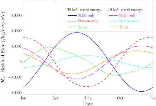
Figure 1: The modulation due to the Standard Halo Model (SHM) and Sagittarius (Sgr) stream separately, as well as the combined modulation, for a Germanium detector. Each component is shown at a recoil energies of 10 keV and 39 keV. The WIMP mass is assumed to be 60 GeV and the Sgr density is taken to be 5% of the SHM density.

The detector type (composed of an element with mass $M$) and WIMP mass $m$ arise in Eqn. (24) only through a constant scaling of the parameter $x=\frac{v_{\textrm{min}}}{\overline{v}_{0}}$ with the square root of the recoil energy $E$ via Eqn. (3). Thus, the modulation behavior of Eqn. (24) and the two features listed above are expected to be observed in any detector, for any WIMP mass, but at different energy scales. For the sake of illustration, we will assume a WIMP mass $m=60$ GeV and a Germanium ($A\approx 73$) detector. In this case $x=0.25\sqrt{E/1\textrm{keV}}$; the parameter value of $x_{p}$ = 0.89 at which the phase of the modulation reverses in Eqn. (24) corresponds to an energy $E_{p}=13$ keV. Then for $E<13$ keV, there will be a cosine-like modulation in the recoil rate at the few percent level, minimized around June 1; see Figure 1 for an example. For $13$ keV $<E<110$ keV, a cosine-like modulation will occur, but will be maximized around June 1; again see Figure 1. For $E\lower 2.0pt\hbox{$\,\buildrel\scriptstyle>\over{\scriptstyle\sim}\,$}110$ keV, the overall rate becomes insignificantly small (compared to lower energies). Experiments such as CDMS Akerib:2005kh and EDELWEISS Sanglard:2005we , which use Germanium detectors, have thresholds low enough to potentially see this phase reversal, but are not expected to observe enough events to discern the small (few percent) modulation effect. Experiments using other elements in their detectors, such as ZEPLIN Alner:2005pa and XENON Aprile:2004ey (using Xenon), likewise could see such a reversal if the exposure is sufficient to detect the modulation effect.

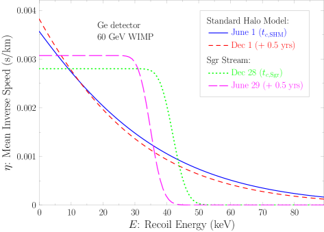
Figure 2: The mean inverse speed $\eta$, given by Eqn. (2), for the SHM and Sgr stream at $t_{c}$ and $t_{c}$ + 0.5 years, where $t_{c}$ is different for the two WIMP populations. The characteristic time $t_{c}$ is the time of year at which the Earth is moving fastest relative to the given WIMP population (see Section II.3). For the SHM, $\eta$ at $t_{c,\textrm{SHM}}$ (June 1) is slightly larger at higher recoil energies and smaller at lower recoil energies than at $t_{c,\textrm{SHM}}$ + 0.5 years (Dec 1); the change in the phase occurs at an energy $E_{p,\textrm{SHM}}$ = 13 keV. In the SHM, the fractional change in $\eta$ is of order $\frac{V_{\oplus}}{v_{\odot,\textrm{SHM}}}$ (only a few percent) for all energies. For the Sgr stream at $t_{c,\textrm{Sgr}}$ (Dec 28), $\eta$ is flat up to a cutoff near the characteristic energy $E_{c,\textrm{Sgr}}$ = 39 keV (see Eqn. (28)); the cutoff is softened by the velocity dispersion of WIMPs in the stream. At $t_{c,\textrm{Sgr}}$ + 0.5 years (June 29), the cutoff energy has decreased to around 35 keV due to the lower maximum WIMP velocities, but the plateau height at energies below this has increased relative to $t_{c,\textrm{Sgr}}$. For $\eta$ at energies below the cutoff, the relative change over the year is also of order $\frac{V_{\oplus}}{v_{\odot,\textrm{SHM}}}$. However, due to the shift in the cutoff, the change in $\eta$ is not suppressed by this velocity factor over a small range of recoil energies near 39 keV; the change here is $\mathcal{O}(1)$ relative to the average at that energy.

Both features, the small modulation amplitude and phase change, arise predominantly from the mean inverse speed factor $\eta$ in Eqn. (1); $\eta$ is shown in Figure 2 at both $t_{c}$ and $t_{c}$ + 0.5 years. At $t_{c}$, the Earth is moving the fastest relative to the SHM, shifting the WIMP velocity distribution, Eqn. (10), to higher velocities compared to $t_{c}$ + 0.5 years (when the Earth is moving slowest). The total recoil rate (over all energies) is highest at $t_{c}$, but the shift to higher velocities depletes the number of low velocity WIMPs and low energy recoils. However, the small change in our velocity throughout the year relative to our velocity through the SHM, along with the large velocity dispersion of WIMPs (comparable to our motion through the halo), yield only small changes in $\eta$; the fractional change is of order $\frac{V_{\oplus}}{v_{\odot,\textrm{SHM}}}$ for all energies. The large velocity dispersion reduces the modulation effect because, even in our frame, there are significant numbers of WIMPs incident on Earth from all directions (but somewhat more likely from the “forward” direction): in some directions, the WIMP velocity is actually reduced at $t_{c}$ and increased at $t_{c}$ + 0.5 years. The geometrical factor $b$ in Eqn. (16) (relating to the angle of the Sun’s motion through the galaxy with the Earth’s orbital plane), here having the value 0.49, further suppresses the modulation amplitude.

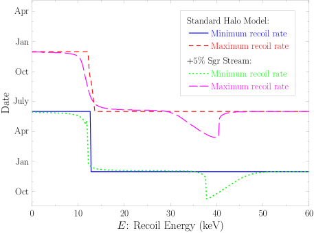
Figure 3: The dates at which the minimum and maximum recoil rates occur for various recoil energies. For the SHM alone, as demonstrated in Figure 1, the modulation is symmetric about $t_{c,\textrm{SHM}}$ (June 1), with a minimum at this time for energies below $E_{p,\textrm{SHM}}$ = 13 keV and a maximum here for energies above this; the other extremum is always at $t_{c,\textrm{SHM}}$ + 0.5 years (Dec 1). The Sgr stream component alone is symmetric about $t_{c,\textrm{Sgr}}$ (Dec 28); but when the SHM and Sgr stream are combined (shown here with a 5% stream density relative to the SHM density), the total modulation becomes asymmetric. The asymmetry is apparent at 30-50 keV, where the maxima and minima are not 0.5 years apart.

As is apparent from Eqn. (24), the modulation is symmetric in time about $t_{c}$ (June 1) for the SHM. The rate is always at an extremum on this date, with the other extremum 0.5 years later (Dec 1), as seen in Figure 3. We shall see in the next section that there is no symmetry when additional WIMP populations, such as streams, are present in the halo: the date of the rate extrema changes with energy and the minimum and maximum rate need not occur 0.5 years apart.

IV Sagittarius Stream

Beyond the smooth SHM dark matter distribution, the galaxy contains additional structure, such as streams arising from late infall of dark matter or tidal disruption of dwarf galaxies being absorbed by the Milky Way. While we are interested in examining streams in general, in this section we will use the Sagittarius (Sgr) stream Yanny:2003zu ; Newberg:2003cu ; Majewski:2003ux as an example to illustrate how various stream parameters affect the modulation signal in a detector. As discussed previously, the Sgr stream is a stream of WIMPs associated with a tidally stripped tail of the Sgr dwarf galaxy that is currently being absorbed by our galaxy. This tidal tail passes through the Milky Way’s disk very near to us, so the WIMPs in the Sgr stream are potentially observable in direct detection experiments. Detection of WIMPs from the Sgr stream has been discussed in Refs. Freese:2003na ; Freese:2003tt ; here, we expand upon those discussions. We will discuss the dependence of the annual modulation in the count rate on the recoil energy, the binning of the recoil energy, the stream density, and the stream dispersion. In Section V, we will examine how the results illustrated with the Sgr stream can change with more general streams. From the parameters discussed in Section II.2 and Section II.3, the characteristic time for this WIMP population, i.e. the date at which we are moving fastest relative to the stream, is $t_{c}$ = 0.991 (Dec 28). The geometric parameter $b$ in Eqn. (16), associated with the angle of the stream relative to the Earth’s orbital plane, is equal to 0.53.

We first examine the basic behavior of a stream by neglecting the velocity dispersion ($\sigma_{v}=0$). In this case, the mean inverse speed $\eta$, Eqn. (2), has the constant value $\frac{1}{v_{\textrm{obs}}(t)}$ up to a cutoff energy $E_{\textrm{co}}(t)$,

$$\eta(E,t)=\frac{1}{v_{\textrm{obs}}(t)}\theta\left[E_{\textrm{co}}(t)-E\right]\,,$$ (25)

where $\theta$ is the Heaviside step function. The cutoff energy corresponds to $v_{\textrm{min}}=v_{\textrm{obs}}(t)$ (see Eqn. (3)), so

$$E_{\textrm{co}}(t)=E_{c}\left[1+A_{c}\cos{\omega(t-t_{c})}\right]\,,$$ (26)

where

$$A_{c}\equiv\frac{2\,b\,v_{\odot,\textrm{Sgr}}V_{\oplus}}{v_{\odot,\textrm{Sgr}}^{2}+V_{\oplus}^{2}}.$$ (27)

We define a characteristic energy

$$E_{c}\equiv\frac{2\mu^{2}}{M}\langle\left[v_{\textrm{obs}}(t)\right]^{2}\rangle=\frac{2\mu^{2}}{M}\left(v_{\odot,\textrm{Sgr}}^{2}+V_{\oplus}^{2}\right)\,.$$ (28)

The relevant velocities have been defined in Section II.3 (see, e.g., Eqns. (20) and (21)). The characteristic energy $E_{c}$ is also the average cutoff energy for the case of zero velocity dispersion discussed here, but the definition in Eqn. (28) may still be used when a velocity dispersion is included ($\sigma_{v}\neq 0$; see below), in which case there is no hard cutoff energy at $E_{\textrm{co}}(t)$. While this definition can also be used to define an $E_{c}$ for any WIMP population, $E_{c}$ is not a useful quantity for a WIMP population with a large velocity dispersion ($\sigma_{v}\lower 2.0pt\hbox{$\,\buildrel\scriptstyle>\over{\scriptstyle\sim}\,$}v_{\odot}$), such as the SHM, as there is no associated rapid drop off in the count rates near that energy such as with a stream (which has $\sigma_{v}\ll v_{\odot}$). Hence, we will only use the characteristic energy of streams in our discussion. We wish to emphasize the importance of the step function in Eqn. (25): the presence of the step and the fact that its position varies with time have key consequences that will be seen in the discussion that follows.

As with the SHM modulation discussed in the previous section, the modulation from the stream (arising from Eqn. (25)) occurs for any detector type, composed of an element with mass $M$, and any WIMP mass $m$. However, the characteristic energy $E_{c}$ given by Eqn. (28) and, thus, the location of the step as given by Eqn. (26) depend explicitly on $M$ and $m$ (recall $\mu\equiv Mm/(M+m)$ is the reduced mass). The choice of $M$ and $m$ do not change the qualitative behavior of the modulation, only the energy scales at which various effects occur. For illustrative purposes, we take a $60$ GeV WIMP and a Germanium detector, for which $E_{c}$ = 39 keV for the Sgr stream; our results will apply to other detectors and WIMP masses, just at different energies.

For the dispersionless case,

$$\chi_{m}(E,t)\approx-0.046\,\cos{\omega(t-t_{c})}\,,\quad\quad\textrm{for}\,\,E<E_{\textrm{co,min}}$$ (29)

and there are no recoils for $E>E_{\textrm{co,max}}$, where $E_{\textrm{co,min}}$ and $E_{\textrm{co,max}}$ are the minimum and maximum cutoff energies, occurring at $t_{c}$ + 0.5 years and $t_{c}$, respectively. Below $E_{\textrm{co,min}}$, the relative variation in the recoil rate is of order $\frac{V_{\oplus}}{v_{\odot,\textrm{Sgr}}}$ and the modulation of the rate is cosine-like with a minimum at $t_{c}$; this behavior is similar to that seen in the SHM for energies below the phase reversal energy $E_{p}$. For $E>E_{\textrm{co}}(t)$, the WIMPs in the stream are not moving sufficiently fast to produce a recoil of energy $E$. However, for $E_{\textrm{co,min}}<E<E_{\textrm{co,max}}$, there are times during the year at which $E>E_{\textrm{co}}(t)$ ($\mathcal{R}=0$) and there are times at which $E<E_{\textrm{co}}(t)$ ($\mathcal{R}>0$). In this case, the size of the modulation is $\mathcal{O}(1)$ relative to the average recoil rate due to the step in Eqn. (25), much larger than the $\mathcal{O}(\frac{V_{\oplus}}{v_{\odot,\textrm{Sgr}}})$ effect arising from the time dependence in $\frac{1}{v_{\textrm{obs}}(t)}$ that is apparent in Eqn. (18); the modulation in this energy range can be quite large and non- cosine-like.

The behavior of Eqn. (25) approximately holds for non-zero velocity dispersion $\sigma_{v}$ as well, provided the dispersion is not significantly larger than the changes in $v_{\textrm{obs}}(t)$ (i.e. $\sigma_{v}\lower 2.0pt\hbox{$\,\buildrel\scriptstyle<\over{\scriptstyle\sim}\,$}bV_{\oplus}$), although the cutoff softens for non-zero $\sigma_{v}$. For illustrative purposes, we take the velocity dispersion of Eqn. (7) to be $\sigma_{v}$ = 25 km/s for the Sgr stream (corresponding to $\overline{v}_{0}$ = 20 km/s from Eqn. (9)), although we will examine variations in this parameter in Section IV.5. For this case, $\eta$ is shown in Figure 2 at both $t_{c}$ (Dec 28) and $t_{c}$ + 0.5 years (June 29). In the figure, the softened step function is apparent, with a cutoff around $E_{c}$ = 39 keV. The height of the step and the cutoff energy vary with time. At $t_{c}$, the Earth is moving the fastest relative to the stream. This leads to a larger range of recoil energies as opposed to $t_{c}$ + 0.5 years, when the Earth is moving the slowest, so the step occurs at a larger energy at $t_{c}$ ($\sim$43 keV) than half a year later ($\sim$35 keV). The higher WIMP velocities, by spreading the recoils over a larger energy range, lead to less recoils at any given energy and a lower step height. The relative variation in the step height is of order $b\,\frac{V_{\oplus}}{v_{\odot,\textrm{Sgr}}}$ ($\sim$5%), similar to the relative variation in $\eta$ for the SHM (also a few percent). However, the variation around the step is unlike any seen in the SHM: $\eta$ goes from nearly zero at $t_{c}$ + 0.5 years to essentially the full step height at $t_{c}$. Just as with the dispersionless case previously discussed, the dominant contribution to the modulation in this energy range is the shift on and off the step, not the variation in the step height itself. Thus, the relative variation in the recoil rate (recall $\mathcal{R}(t)\propto\eta(t)$) is not suppressed by the above velocity factor and $\chi_{m}\sim\mathcal{O}(1)$. This is a large amplification in the signal and could potentially yield an observable signal for the Sgr stream at a comparable level to the SHM, even if the Sgr stream is significantly less dense.

To examine the recoil rate for the Sgr stream and compare to the SHM, we must assume a local density $\rho_{\textrm{Sgr}}$ for the stream. For illustrative purposes, we will assume a stream density 5% that of the SHM ($\rho_{\textrm{Sgr}}=0.05\rho_{\textrm{SHM}}$). We note this is optimistic and that the local Sgr density is likely at most a few percent Freese:2003tt . However, 5% is not unreasonable for other structure in the dark matter distribution, such as clumps Stiff:2001dq . The various effects we examine still mainly apply for lower densities, just to smaller degrees. We will, however, examine variations in the density in Section IV.4.

We will take $\rho_{\textrm{Sgr}}=0.05\rho_{\textrm{SHM}}$ and $\sigma_{v}=$ 25 km/s to be our fiducial values in Sections IV.1-IV.3 and then we will vary them in Sections IV.4 & IV.5, respectively. We will examine the dependence of the modulation in the count rate as a function of the recoil energy, the binning of the recoil energy, the stream density, and the stream dispersion. We wish to reiterate the following definitions, which play an essential role in the remaining discussions:

the characteristic time $t_{c}$

is the time of year at which Earth is moving fastest relative to some WIMP population, formally defined by Eqn. (17), and

the characteristic energy $E_{c}$

is the approximate energy at which a rapid drop in the recoil rate occurs for streams, formally defined by Eqn. (28).

We also reiterate that, for illustrative purposes, we take a $60$ GeV WIMP and a Germanium detector, for which $E_{c}$ = 39 keV for the Sgr stream; our results will apply to other detectors and WIMP masses, just at different energies.

IV.1 Contrasting and Summing the Halo and Stream Modulations

Here we will compare the modulation due to a stream, using the Sgr stream as an example, with the modulation due to the SHM as discussed in Section III and we will examine the total modulation (sum of the SHM and stream components) that a detector will observe. Figures 1-3 demonstrate out results.

For a 5% Sgr stream with $\sigma_{v}$ = 25 km/s, the residual rate (modulation) is shown in Figure 1 at recoil energies of 10 keV and 39 keV. At 10 keV, the modulation is essentially a cosine minimized on December 28 ($t_{c,\textrm{Sgr}}$) and maximized on June 29. This behavior is similar to the low energy behavior of the SHM, although the SHM has a different $t_{c}$ (June 1) and, hence, does not peak at the same time. At 39 keV, near the characteristic energy $E_{c,\textrm{Sgr}}$ for the Sgr stream, we see the modulation becomes extremely large for the stream, with an amplitude nearly four times larger than at 10 keV, even though the nuclear form factor in Eqn. (4) generally causes the recoil rate to decrease at higher energies. This amplification in the amplitude is due to the $\eta$ step edge crossing discussed previously. The phase at 39 keV is reversed from that at 10 keV: the maximum now occurs on December 28 ($t_{c,\textrm{Sgr}}$) rather than on June 29. However, unlike the SHM, the stream modulation is not cosine-like at all energies. While this particular instance may look somewhat cosine-like, most energies in the cutoff range around $E_{c}$ are decidedly not cosine-like; a smaller $\sigma_{v}$ would also make the modulation at $E_{c,\textrm{Sgr}}$ less cosinusoidal (we shall see this in Section IV.5).

In general, even if the WIMP population components (e.g. SHM and Sgr stream) individually produce cosinusoidal modulations, the total modulation seen in detectors is not cosinusoidal. At 10 keV, the total modulation shown in Figure 1 does look somewhat cosinusoidal; this, however, is a coincidence due to the nearly six month difference between the $t_{c}$’s of the two components. At $E_{c,\textrm{Sgr}}$ = 39 keV, the total modulation is clearly not time-symmetric.

While the SHM and Sgr stream always have their maxima or minima at their respective $t_{c}$’s for any energy (but possibly changing between the maximum and minimum at some specific energy), the combined modulation has extrema occurring on dates that vary with energy. In Figure 3, the SHM can be seen to always have the extrema on June 1 ($t_{c,\textrm{SHM}}$) and December 1, but with the extrema reversing at an energy $E_{p,\textrm{SHM}}$ = 13 keV. With a 5% stream in addition to the SHM, the combined modulation is mostly the same as for the SHM alone except near $E_{p,\textrm{SHM}}$ and $E_{c,\textrm{Sgr}}$. At low energies ($E\lower 2.0pt\hbox{$\,\buildrel\scriptstyle<\over{\scriptstyle\sim}\,$}8$ keV), the SHM has the most significant contribution to the modulation and the extrema occur on nearly the same dates as the SHM alone. At intermediate energies (15 keV $\lower 2.0pt\hbox{$\,\buildrel\scriptstyle<\over{\scriptstyle\sim}\,$}E\lower 2.0pt\hbox{$\,\buildrel\scriptstyle<\over{\scriptstyle\sim}\,$}$ 30 keV), the SHM is again the most significant component and the extrema of the total modulation are near that of the SHM’s. Above 45 keV (above the maximum cutoff energy $E_{\textrm{co,max}}$ for the Sgr stream), there is essentially no contribution from the stream, so the extrema match the SHM. In the regions near $E_{p,\textrm{SHM}}$ and $E_{c,Sgr}$, however, the dates at which the maximum and minimum count rates occur are different for the combined SHM & Sgr stream modulation than they would be for the SHM alone. The SHM modulation amplitude varies smoothly across zero at $E_{p,\textrm{SHM}}$ and is small at nearby energies, as can be seen in Figure 2. The Sgr stream modulation amplitude does not vary significantly at these energies, so the stream contributes significantly to the modulation and leads to a smooth variation in the extrema dates. Around and between $E_{\textrm{co,min}}$ and $E_{\textrm{co,max}}$ for the stream (33-45 keV), the total modulation fluctuates wildly due to the cutoff in $\eta$. The modulation here is noticeably asymmetric in Figure 3, as the extrema are not 0.5 years apart.

As noted above, several properties can emerge from multiple components that are not present in the individual components:

• The combined modulation is generally non-cosinusoidal, even if the modulation of each individual component is;

• The combined modulation need not be time-symmetric, even if each individual components is; and

• The minimum and maximum recoil rates need not occur 0.5 years apart.

These three effects, if observed, are potentially evidence for some structure (streams) in the local WIMP population. These effects will be apparent in the following sections, as we examine the behavior of the modulation for different recoil energies, recoil energy binning, stream density, and stream dispersion. For these sections, we will be examining only the combined modulation of the SHM and Sgr stream (not individually).

IV.2 Recoil Energy

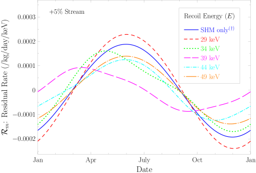
Figure 4: Dependence on recoil energy. The solid (blue) line shows the modulation due to only the SHM at a recoil energy of 39 keV $({\dagger})$; the remaining lines include a 5% Sgr stream in addition to the SHM at various recoil energies. The shape of the modulation is dependent on the recoil energy and clearly exhibits non- cosine-like behavior over a range of energies. The contribution from the stream falls off at energies above 39 keV, the characteristic energy $E_{c,\textrm{Sgr}}$ for the Sgr stream (see Figure 2).

Here we discuss the dependence of the total modulation on the recoil energy. As seen in Figure 4, the shape of the modulation is highly dependent on this energy. In this figure, we have chosen to show the total modulation at representative energies below, at, and above 39 keV, the characteristic energy of the Sgr stream for 60 GeV WIMPs in a Germanium detector. For comparison, the cosine-like contribution from the SHM alone is shown at 39 keV (solid/blue line).

Well below the characteristic energy of the stream, both the SHM and stream modulations are cosine-like, although peaking at different times. In Figure 4, we see that the combination is approximately cosine-like at 29 keV, a consequence of the two separate modulations being nearly in phase with each other (both the SHM and Sgr stream peak in the summer at this energy). For the SHM (and other WIMP populations), the cosine-like modulation comes from the expansion of the SHM’s speed relative to the Earth $v_{\textrm{obs}}(t)$ in the powers of $\frac{V_{\oplus}}{v_{\odot}}\ll 1$ as given in Eqn. (18). This equation has corrections of $\mathcal{O}(\frac{V_{\oplus}^{2}}{v_{\odot}^{2}})$. Although not noticeable in the figure, the combined SHM + Sgr stream modulation at 29 keV differs from a true cosine by a larger amount than these $\mathcal{O}(\frac{V_{\oplus}^{2}}{v_{\odot}^{2}})$ corrections. A stream with a different $t_{c}$ would yield a modulation that does not appear as cosine-like.

At 39 keV ($E_{c,Sgr}$), the $\mathcal{O}(1)$ relative modulation of the stream leads to a contribution to the modulation by the stream comparable in magnitude to the contribution from the SHM, shifting the peak date by nearly three months and greatly decreasing the modulation amplitude relative to the SHM dominated behavior at 29 keV or SHM component of the modulation alone at 39 keV. This is a highly significant result: even though the stream is much less dense than the SHM, its modulation is just as large as that of the SHM here. The stream’s effect on the total modulation is likely to be seen here well before other energies. The asymmetry in the modulation is apparent at this energy. The contribution to the total modulation from the stream is also significant at energies near to $E_{c,\textrm{Sgr}}$, as can be seen at 34 keV and 44 keV (the latter being more apparent near the minima in the figure).

At 49 keV, above $E_{\textrm{co,max}}$ for the stream, there is essentially no contribution from the stream and the total modulation assumes the cosine-like form of the SHM. The amplitude is reduced from the case at 29 keV, which had contributions from the stream, and is also slightly smaller than the SHM component alone at 39 keV, due to the form factor in Eqn. (4) that lowers the count rate at higher energies.

A stream can have a significant effect on the modulation near the characteristic energy $E_{c}$ even if the stream is far less dense than the smooth background halo distribution (here, the SHM). The stream can significantly change the peak date and the shape of the modulation (becoming quite non-cosinusoidal) near this energy. Away from this energy, however, a low density stream has only a mild impact, if any, on the modulation. The question of how well experiments are able to distinguish the modulation behavior near $E_{c}$, due to the limited energy resolution in a detector, is addressed in the following section.

IV.3 Recoil Energy Range (Binning)

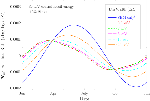
Figure 5: Dependence on binning of recoil energy. The average modulation observed over an energy range centered at 39 keV ($E_{c,\textrm{Sgr}}$) with a width $\Delta E$. The solid (blue) line is for the SHM only with zero bin width $({\dagger})$; the remaining lines include a 5% Sgr stream in addition to the SHM. Only for large bins, $\Delta E\lower 2.0pt\hbox{$\,\buildrel\scriptstyle>\over{\scriptstyle\sim}\,$}10$ keV, does the shape of the modulation differ significantly from that of the differential recoil rate (equivalent to zero bin width: $\Delta E=0$ keV).

We examine how the modulation appears when averaged over some range of recoil energies, as would be observed when experimental data is binned, and demonstrate the results in Figure 5. We have seen that the Sgr stream has a significant effect on the modulation at least over the recoil energy range 34-44 keV (see Figure 4). As detectors have limited energy resolution, experimental results are often binned in recoil energies. If the bins are much larger than the limited width of the stream’s $\mathcal{O}(1)$ relative modulation effect, it would be difficult to study this behavior or even observe it. In Figure 5, the modulation from the SHM and a 5% Sgr stream is shown for multiple bin sizes ($\Delta E$), where the bins are centered at 39 keV, the characteristic energy $E_{c,\textrm{Sgr}}$ (corresponding the energy cutoff; see Figure 2). The average recoil rate,

$$\langle\mathcal{R}\rangle=\frac{1}{\Delta E}\int_{E_{c}-\Delta E/2}^{E_{c}+\Delta E/2}\mathcal{R}(E)\,\mathrm{d}E\,,$$ (30)

is used in each case. For comparison, the SHM component alone is shown at 39 keV.

An infinite resolution detector, with $\Delta E$ = 0, will observe the actual recoil rate at $E_{c,\textrm{Sgr}}$. For bin widths of 2 & 5 keV, there is very little deterioration in the modulation signal. Even for a 10 keV bin, the modulation signal is similar to the $\Delta E$ = 0 case. For $\Delta E$ = 20 keV, the signal is highly deteriorated, but the modulation observed is still very different from the SHM case. The current generation of Ge detectors have energy resolutions on the order of 1-2 keV, so it is clear detector resolution will not inhibit observation of the stream’s effect on the modulation around $E_{c,\textrm{Sgr}}$.

IV.4 Stream Density

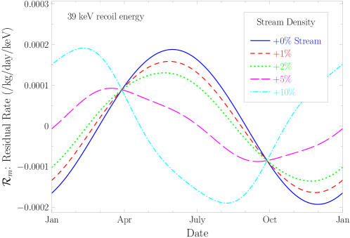
Figure 6: Dependence on stream density. The modulation for a variety of stream densities at a recoil energy of 39 keV ($E_{c,\textrm{Sgr}}$); stream densities are given relative to the (fixed) SHM density. The solid (blue) line represents the SHM alone. Even at only 5% of the density, the stream has a comparable modulation amplitude to that of the SHM alone near the cutoff energy, yielding a total modulation quite different than would be expected for the SHM alone.

The extent to which a stream affects the annual modulation depends upon the density of the stream. The modulation due to the SHM + Sgr stream is shown in Figure 6 for several different stream densities, all at the characteristic energy $E_{c,\textrm{Sgr}}$. For comparison, the SHM only case is shown by the solid (blue) line. At this energy, the modulation of the SHM peaks on June 1; that of the Sgr stream is minimized on June 29. The stream obviously significantly contributes to the overall modulation at this energy for the 5% relative density we have been using.

While a 5% density may be reasonable for some streams Stiff:2001dq (the caustic ring model of P. Sikivie and collaborators predicts a stream as large as 75% of the local density; see Ref. Ling:2004aj and references therein), it is optimistically large for the Sgr stream. Instead, a density of a few percent or lower may be more reasonable. Would such low densities be observable? In the figure, streams at 5% and 10% densities differ significantly from the SHM component. In these cases, the modulation is non-cosinusoidal and asymmetric and has a different amplitude and peak date than the SHM component. For the 5% case, the maximum rate occurs 3 months prior to that of the SHM component. For a 2% stream, the modulation shape and peak date do not differ significantly from that of the SHM. However, even though the stream density is only $1/50$ that of the SHM, the amplitude of the total modulation is still decreased by more than 30% from that of the SHM alone near $E_{c,\textrm{Sgr}}$. The implication then is, due to the $\mathcal{O}(1)$ relative modulation of the stream near $E_{c,\textrm{Sgr}}$, a relatively small stream can still have a significant effect on the experimental results.

IV.5 Stream Dispersion

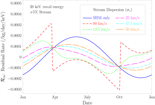
Figure 7: Dependence on stream dispersion. The modulation at ($E_{c,\textrm{Sgr}}$) is shown for various stream velocity dispersions ($\sigma_{v}$). The solid (blue) line is for the SHM only; the remaining lines include a 5% Sgr stream in addition to the SHM. For $\sigma_{v}=0$ km/s, the stream has a step function contribution on top of the cosine-like modulation of the SHM. Increasing velocity dispersion softens the step function like behavior.

We examine the dependence of the modulation on the velocity dispersion $\sigma_{v}$ of the stream, illustrated in Figure 7. Up to this point we have taken the dispersion to be 25 km/s, and we now allow it to vary. The SHM and Sgr stream have very different modulation behaviors: the SHM modulation is always very nearly cosinusoidal, with a small amplitude and a reversal of the modulation phase at an energy $E_{p,\textrm{SHM}}$. The stream modulation, on the other hand, has three different behaviors: it is cosinusoidal with a small amplitude at energies below the characteristic energy $E_{c,\textrm{Sgr}}$, it is large ($\mathcal{O}(1)$ relative to the average rate) and non-cosinusoidal around $E_{c,\textrm{Sgr}}$, and it is non-existent above this energy. The differences between these two components are mainly due to the large difference in their velocity dispersions, leading to the following two consequences: (1) For a dispersion of a WIMP population significantly smaller than the net motion $v_{\textrm{obs}}$ of that population relative to a detector, or $\sigma_{v}\ll v_{\odot}$, the recoil energy spectrum develops a relatively rapid drop near the characteristic energy $E_{c}$ (true for the Sgr stream but not for the SHM). (2) For a dispersion on the order of the variation in $v_{\textrm{obs}}(t)$ due to the Earth’s orbital motion, or $\sigma_{v}\lower 2.0pt\hbox{$\,\buildrel\scriptstyle<\over{\scriptstyle\sim}\,$}bV_{\oplus}$, the variation of the location of this dropoff leads to relatively large, non-cosinusoidal modulations in the count rates near $E_{c}$ (again, this applies to the Sgr stream but not the SHM). This second condition essentially requires that the shift in the location of the step ($\sim bV_{\oplus}$) be comparable or larger than the width of the step dropoff itself ($\sim\sigma_{v}$); if this condition is not satisfied, the modulation near $E_{c}$ remains a relatively small effect (only a few percent of the total rate, as occurs at other energies). While the presence of a dropoff is signified by the condition of (1), the (usually) stronger condition of (2) is necessary to make the dropoff rapid enough to observe the large modulation effect.

For the stream, $\eta(E)$ is similar to a step function, with the position of the step, Eqn. (26), shifting in time; see Figure 2. The shift in the step is proportional to $bV_{\oplus}$, the change in stream velocity $v_{\textrm{obs}}(t)$ (recall $0\leq b\leq 1$ is a geometrical factor dependent upon the stream direction). The edge of the step, however, is softened, with the fall off occurring over an energy range proportional to $\sigma_{v}$. As long as the velocity dispersion is not significantly larger than the changes in $v_{\textrm{obs}}(t)$ (i.e. $\sigma_{v}\lower 2.0pt\hbox{$\,\buildrel\scriptstyle<\over{\scriptstyle\sim}\,$}bV_{\oplus}$), the edge is sharp enough so that, at some energies, a large portion of the edge crosses the given energy throughout the year. Note how in Figure 2, $\eta$ is nearly atop the step at 39 keV on December 28 ($t_{c,\textrm{Sgr}}$) for the Sgr stream, but is beyond the step on June 29. When $\sigma_{v}\gg bV_{\oplus}$, the step is washed out, as can be seen by $\eta$ for the SHM in the same figure. The small dispersion that is a characteristic of streams leads to the $\mathcal{O}(1)$ relative modulation (arising from the crossing of the step) that is not present in the SHM with its large dispersion.

The SHM + 5% Sgr stream modulation is shown in Figure 7 for multiple stream dispersions at a recoil energy of 39 keV ($E_{c,\textrm{Sgr}}$). For comparison, the SHM only case is again shown by the solid (blue) line. The step like behavior in $\eta$ for the stream is apparent as the dispersion goes to zero. At $\sigma_{v}=0$, where $\eta$ is a true step function, the step edge, $E_{\textrm{co}}$, can be seen to have cross 39 keV in late March and early October. From March to October, the stream cutoff energy is below the recoil energy being observed, so that the stream does not contribute to the count rate (note how the shape of the modulation on these dates is identical to the SHM only component). From October to April, the cutoff energy is above the recoil energy being observed, so the stream also contributes to the count rate.

As $\sigma_{v}$ increases, the sharp changes in the modulation in March and October are softened. $\sigma_{v}$ = 12.5 km/s still looks somewhat similar to the $\sigma_{v}=0$ case. The $\sigma_{v}$ = 25, 37.5, & 50 km/s cases all have $\sigma_{v}$ greater than $bV_{\oplus}$ = 16 km/s; the abrupt changes in the recoil rate are now gone. However, $\sigma_{v}$ is not significantly larger than $bV_{\oplus}$ and an appreciable portion of the $\eta$ step still crosses this recoil energy: the lighter stream still has an effect on the modulation comparable to that of the SHM, as evident by the large difference between these cases and the SHM only case.

As noted by Refs. Stiff:2001dq ; Helmi:1999ks ; Helmi:1999uj , the stream’s velocity dispersion is more likely to be anisotropic, in which case the distribution of Eqn. (7) is not valid. However, including anisotropic models of the stream’s velocity distribution would not significantly affect the results discussed in this paper as the velocity dispersion of the stream will still be significantly smaller than the stream velocity relative to the observer. In such models, the dropoff in the recoil rate would still be present, as well as a modulation of both the recoil rate and location of the dropoff. Including such models would simply lead to modest changes in the shape of the dropoff in the mean inverse speed (see Figure 2) and, hence, the recoil rate around the characteristic energy $E_{c}$.

V General Streams

Having examined various stream parameters using the Sgr stream in the previous section, we wish to expand our results to streams in general. The Sgr stream modulation features previously discussed likewise occur for other streams: (1) The phase of the stream modulation is associated with a characteristic time $t_{c}$ (typically the time of year at which the recoil rate is maximized or minimized) that is independent of the SHM; (2) There exists a characteristic energy $E_{c}$ associated with a rapid dropoff to zero in the recoil rate; (3) At energies less than the characteristic energy $E_{c}$, the modulation is nearly cosinusoidal, with a minimum at $t_{c}$ and a (small) amplitude of $\mathcal{O}(\frac{V_{\oplus}}{v_{\textrm{obs}}})$ with respect to the average rate; and (4) The modulation near $E_{c}$ is not cosinusoidal, is of $\mathcal{O}(1)$ relative to the average rate, and can be comparable in amplitude to that of the overall halo modulation. While any stream will have these features (we are assuming a small velocity dispersion, or $\sigma_{v}\lower 2.0pt\hbox{$\,\buildrel\scriptstyle<\over{\scriptstyle\sim}\,$}V_{\oplus}$, as would be expected for typical streams), the characteristic time $t_{c}$ and energy $E_{c}$ depend upon the stream. Given a stream velocity $\mathbf{v}_{\odot,\textrm{str}}$, these values may be determined from Eqn. (17) and Eqn. (28), respectively (using $v_{\odot,\textrm{str}}$ in place of $v_{\odot,\textrm{Sgr}}$ in the latter equation). We will examine how the stream speed and direction affect the characteristic time and characteristic energy, and consequently the modulation.

V.1 Stream Speed

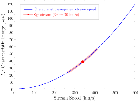
Figure 8: Stream speed. The characteristic energy $E_{c}$, defined by Eqn. (28), as a function of stream speed. $E_{c}$ is approximately the highest possible recoil energy from a WIMP in the stream. $E_{c}$ is independent of the stream direction and depends only on the speed of the stream relative to the Sun ($v_{\odot,\textrm{str}}$; solid/blue line). The $340\pm 70$ km/s speed of the Sgr stream is shown (red dot with wide pink line indicating the $1\sigma$ region), corresponding to an $E_{c}$ range of 25-55 keV with central value 39 keV.

The characteristic energy $E_{c}$ of a stream, Eqn. (28) with $v_{\odot,\textrm{Sgr}}$ replaced with a more general stream speed $v_{\odot,\textrm{str}}$, is dependent only upon the speed of the stream relative to the Sun and is independent of the stream direction. For a stream moving much faster than Earth’s orbital velocity ($v_{\odot,\textrm{str}}\gg V_{\oplus}$), the characteristic energy is proportional to the square of the stream speed relative to the Sun ($E_{c}\propto v_{\odot,\textrm{str}}^{2}$), so faster streams rapidly lead to higher $E_{c}$’s; this behavior is demonstrated in Figure 8.

The $E_{c}$ determined from a modulation signal can be used to determine the speed of the stream to an improved degree over that afforded by limited alternative observations. The $300\pm 90$ km/s Sgr stream speed estimate relative to the galactic rest frame, discussed in Refs. Majewski:2003ux ; Freese:2003tt , is not based upon direct observation of Sgr stellar material in the local neighborhood, but on extrapolating stellar stream observations in other areas of the Milky Way, leading to the relatively large uncertainty. The $300\pm 90$ km/s speed relative to the galactic rest frame corresponds to a speed relative to the Sun of $v_{\odot,\textrm{Sgr}}=340\pm 70$ and, hence, to a 25-55 keV range of $E_{c}$, as shown in Figure 8. This energy range is much larger than the energy resolution of a WIMP detector; current detector resolutions of $\sim$1 keV would yield a stream speed accurate to about $\pm$10 km/s (in the Sgr stream case). To derive the stream speed from $E_{c}$, using Eqn. (28) (where $M$ is the nuclear target mass and $\mu$ is the WIMP-nucleus reduced mass), the WIMP mass must already be reasonably well known.

V.1.1 Determining the WIMP Mass

Alternatively, if the WIMP mass is unknown, but a dropoff in the recoil rate can be associated with a known stream (known via other observations), the energy at which that dropoff occurs, $E_{c}$, can be used to determine the WIMP mass. For instance, if we observe a dropoff at $E_{c}=30\pm 2$ keV in a Germanium detector and associate it with the Sgr stream (with speed $340\pm 70$ km/s), we would derive a WIMP mass of $48\pm 22$ GeV. If further stellar observations and modelling of the Sgr stream improve the speed uncertainties to $\pm 20$ km/s, the mass determination would improve to $48\pm 7$ GeV. Certainly, the presence of a dropoff in the recoil rate, which does not require a modulation effect to be observed, can provide a useful tool for determining the WIMP mass. However, care must be taken in associating such a dropoff with a specific stream: observation of a 5% density stream through such a dropoff alone cannot be assumed to be due to the Sgr stream rather than some as yet unknown other stream. If we can determine the direction of the stream producing the dropoff in the recoil rate, we have a much stronger basis for associating that stream with a known one. We examine the stream direction in the following section.

V.2 Stream Direction

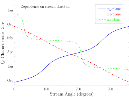
Figure 9: Stream direction. The characteristic time $t_{c}$ as a function of stream direction; $t_{c}$ is independent of the stream speed. Each curve shows the dependence on one of the three angles, in the $xy$-, $xz$-, and $yz$-planes (e.g., the angle $\phi$ in the $xy$-plane corresponds to the direction $\cos\phi\mathbf{\hat{x}}+\sin\phi\mathbf{\hat{y}}$ in Galactic coordinates).

The direction of a stream as well as the speed may be unknown to us. Indeed, a signal in a dark matter detector may even be our first indication of some local stream. The characteristic time $t_{c}$ is dependent only upon the stream direction, via Eqn. (17), so an experimental determination of the former can give us indications of the latter. However, $t_{c}$ alone can only give the direction of the stream in the Earth’s orbital plane about the Sun, insufficient to reconstruct the full stream direction.

The angle of the stream $\lambda_{\odot}$ from the normal of the orbital plane is encoded in the geometrical factor $b$ discussed in Section II.3, with $b=\sin\lambda_{\odot}$. The parameter $b$ can be determined only through modulation effects due to the dependence of $v_{\textrm{obs}}(t)$, Eqn. (16), on the value of $b$. A small value for $b$, corresponding to a stream nearly orthogonal to the orbital plane, yields only small variations in $v_{\textrm{obs}}$ over the course of a year and modulation effects would likewise be small; for a stream perfectly orthogonal to the orbital plane, $v_{\textrm{obs}}$ is constant ($b=0$) and there is no modulation. A large value for $b$, corresponding to a stream incident to the Sun along the Earth’s orbital plane, yields larger variation of $v_{\textrm{obs}}$ and larger modulation effects. The dependence of the modulation on $b$ manifests itself primarily through two effects: the modulation amplitude and the size of the variation in the cutoff energy $E_{\textrm{co,max}}-E_{\textrm{co,min}}$ (see Eqn. (26)), both proportional to $b$. The modulation amplitude is degenerately dependent upon the presumably unknown stream density. The quantity $E_{\textrm{co,max}}-E_{\textrm{co,min}}$ is not, so $b$ can be extracted from a modulation signal (the variation in $E_{\textrm{co}}$ is also dependent upon $v_{\odot}$, which may be unambiguously determined from the cutoff energy as discussed in the previous section).

From $t_{c}$ and $b$, the full direction of the stream may then be determined. In Figure 9, we show $t_{c}$ as a function of angle in the $xy$-, $xz$-, and $yz$-planes (angle is from the first axis indicated in each plane). The characteristic time $t_{c}$ varies most smoothly with angle when the plane is near to that of the orbital plane (the $xz$-plane is the nearest of the three shown). The characteristic time $t_{c}$ changes rapidly in the $yz$-plane (near 30^∘ and 210^∘) when the stream passes near the normal to the orbital plane. The otherwise flat behavior of $t_{c}$ in this case demonstrates how $t_{c}$ is independent of the angle $\lambda_{\odot}$, as the near orthogonality of the $yz$-plane with the orbital plane means rotations in the $yz$-plane correspond strictly to changes in $\lambda_{\odot}$ and not the angle in the orbital plane (except for a 180^∘ phase shift when rotating through the normal to the orbital plane).

The determination of the parameters $t_{c}$ and $b$ from a detector signal is essentially independent of the WIMP mass. Then, even without an understanding of WIMP properties (e.g. mass), we can use these two parameters (by converting them to a stream direction) to associate a dark matter detector signal with possibly visible structure in the galaxy, such as a stellar stream, that is moving in the same directon. Without knowing the WIMP mass or the direction of the stream producing the signal in the detector, a dropoff in the recoil rate spectrum at a characteristic energy $E_{c}$ cannot be associated with any specific known structure (known via other observations), e.g. the Sgr stream, rather than some other unknown stream. As described in the previous section, any visible structure could give an indication of the speed of the dark matter stream and, therefore, lead to a determination of the WIMP mass by the position of the dropoff via Eqn. (28).

V.3 Determination of Stream Parameters

As noted by Stiff, Widrow & Frieman Stiff:2001dq , the modulation signal can be used to determine many of the characteristics of such a stream; we note here that such determinations can be made mainly from a small energy range about $E_{c}$ and, in the following, outline how to do so. The approximate energy of the rapid change in modulation behavior, corresponding to $E_{c}$, yields the stream speed $v_{\odot,\textrm{str}}$ since $E_{c}\propto v_{\odot,\textrm{str}}^{2}$. The location of this cutoff energy varies over the course of a year; the extent of the variation depends upon the geometrical parameter $b$ (the sine of the angle between the stream and the normal to Earth’s orbital plane), which can thus be extracted. From $b$ and the characteristic date $t_{c}$ (the time of year at which the stream moves fastest relative to the Earth; determined from the date of the peak rate), the direction of the stream can be determined via the formulas of Section II.3. The amplitude of the modulation can be used to determine the density of the stream. The width of the cutoff indicates the velocity dispersion in the stream. While observation of these characteristics could potentially be inhibited by limited energy resolutions in dark matter detectors, the resolutions available in some current detectors should be sufficiently high as to not pose a significant impediment to extracting many of these stream parameters.

The various parameters, while all potentially extractable from an observed modulation signal, will not be equally easy to extract. The characteristic energy $E_{c}$, characteristic time $t_{c}$, and stream density $\rho_{\textrm{str}}$ relative to the smooth halo density (assuming the halo modulation is observed at energies not near $E_{c}$) are the parameters most easily extracted from any modulation signal as they have the most dominant effect on such a signal. From the first two of these parameters, two components of the stream velocity can be determined. The stream dispersion $\sigma_{\textrm{str}}$ and the geometrical factor $b$ would be more difficult to extract as they have less significant effects on the modulation signal; extracting these parameters might require much more significant detector exposure and/or a larger detector. The stream dispersion will give an indication of the velocity distribution of WIMPS in the stream, but the interpretation of this parameter should be limited to an approximation of the distribution only as our assumed Maxwellian distribution of Eqn. (7) may not be entirely accurate (see the discussion at the end of Section IV.5). Indeed, directional detectors are likely to be much more useful in characterizing this velocity distribution. From $b$, the third component of the stream velocity can be determined. Alternatively, if a stream is due to a dwarf galaxy being absorbed by the Milky Way, there could be an associated stellar stream that would be indicative of the WIMP stream, yielding independent measurements of the stream velocity. However, for late infall of dark matter clumps and other possible WIMP stream origins, there would be no such stellar stream and WIMP detection alone would be required to characterize the stream parameters.

A stream signal in a dark matter detector may provide a means of determining the WIMP mass, as discussed previously. Individual parameters that play a role in this determination are discussed here. The parameters $E_{c}$, $t_{c}$, and $b$ can be determined from a detector signal without knowing the mass of the WIMP. The latter two parameters would give an indication of the direction of the dark matter stream producing the signal. Knowing this direction, we could associate the dark matter stream with some stellar stream or known structure in the galaxy, such as the Sgr stream, and independently determine the speed of the dark matter stream (which presumably matches that of any visible, e.g. stellar, components). The characteristic energy $E_{c}$ depends only upon the WIMP mass, nuclear target mass, and stream speed, so by knowing the velocity of the stream producing a dropoff in the recoil rate at $E_{c}$, the WIMP mass can be derived (the nuclear target mass is well known in most detectors). The mass determination from a stream in this manner could be more precise than that afforded by the signal from the smooth halo itself.

Detectors that can determine the direction of WIMP induced nuclear recoils are the ultimate goal for characterizing the local WIMP population; however, technology for such a detector is still in the development stage. In the meantime, probing the annual modulation will also allow us to characterize this WIMP population by, e.g., observing the presence of streams in addition to the smooth dark matter halo.

VI Summary

A dark matter stream presents observational signals unlike that of a smooth background distribution (assumed here to be the SHM). The most noticeable difference is the existence of a rapid dropoff in the recoil rate around a characteristic energy $E_{c}$; this dropoff yields a relatively large and non- cosine-like contribution to the annual modulation around $E_{c}$ that may be observable even for a stream much less dense than the SHM. Figure 1 shows the drastic importance the stream can have near $E_{c}$ for the annual modulation. The presence of a rapid change in modulation behavior with respect to recoil energy would be an indication of a stream or other non-SHM component of the dark matter. Since a stream’s effects are mild except near $E_{c}$ (and essentially non-existent well above $E_{c}$), the presence of a stream should not interfere with using the modulation to describe the background distribution, SHM or otherwise. Detection of an annual modulation of the cutoff energy together with the annual modulation of the overall signal provide a “smoking” gun for WIMP detection. In addition, if the WIMP mass is unknown, but a dropoff in the recoil rate can be associated with a known stream (known via other observations), the energy at which that dropoff occurs can be used to determine the WIMP mass.

- (1) R. Bernabei et al., Riv. Nuovo Cim. 26N1, 1 (2003) [arXiv:astro-ph/0307403].
- (2) R. Bernabei et al., Nucl. Phys. Proc. Suppl. 138, 48 (2005).
- (3) G. J. Alner et al. [UK Dark Matter Collaboration], Phys. Lett. B 616, 17 (2005) [arXiv:hep-ex/0504031].
- (4) D. S. Akerib et al. [CDMS Collaboration], Phys. Rev. Lett. 96 011302 (2006) [arXiv:astro-ph/0509259].
- (5) V. Sanglard et al. [The EDELWEISS Collaboration], Phys. Rev. D 71, 122002 (2005) [arXiv:astro-ph/0503265].
- (6) G. J. Alner et al. [UK Dark Matter Collaboration], Astropart. Phys. 23, 444 (2005).
- (7) E. Aprile et al., Nucl. Phys. Proc. Suppl. 138, 156 (2005) [arXiv:astro-ph/0407575].
- (8) G. J. Alner et al., Nucl. Instrum. Meth. A 535, 644 (2004).
- (9) G. J. Alner et al., Nucl. Instrum. Meth. A 555, 173 (2005).
- (10) G. Angloher et al., Astropart. Phys. 18, 43 (2002).
- (11) G. Angloher et al., Astropart. Phys. 23, 325 (2005) [arXiv:astro-ph/0408006].
- (12) T. A. Girard et al., Phys. Lett. B 621, 233 (2005) [arXiv:hep-ex/0505053].
- (13) M. Barnabe-Heider et al. [PICASSO Collaboration], Nucl. Phys. Proc. Suppl. 138, 160 (2005) [arXiv:hep-ex/0312049].
- (14) W. J. Bolte et al., arXiv:astro-ph/0503398.
- (15) A. K. Drukier, K. Freese and D. N. Spergel, Phys. Rev. D 33, 3495 (1986).
- (16) K. Freese, J. A. Frieman and A. Gould, Phys. Rev. D 37, 3388 (1988).
- (17) A. M. Green, Phys. Rev. D 63, 043005 (2001) [arXiv:astro-ph/0008318].
- (18) A. M. Green, Phys. Rev. D 68, 023004 (2003) [Erratum-ibid. D 69, 109902 (2004)] [arXiv:astro-ph/0304446].
- (19) P. Ullio and M. Kamionkowski, JHEP 0103, 049 (2001) [arXiv:hep-ph/0006183].
- (20) N. Fornengo and S. Scopel, Phys. Lett. B 576, 189 (2003) [arXiv:hep-ph/0301132].
- (21) C. J. Copi and L. M. Krauss, Phys. Rev. D 67, 103507 (2003) [arXiv:astro-ph/0208010].
- (22) B. Yanny et al., Astrophys. J. 588, 824 (2003) [Erratum-ibid. 605, 575 (2004)] [arXiv:astro-ph/0301029].
- (23) H. J. Newberg et al., Astrophys. J. 596, L191 (2003) [arXiv:astro-ph/0309162].
- (24) S. R. Majewski, M. F. Skrutskie, M. D. Weinberg and J. C. Ostheimer, Astrophys. J. 599, 1082 (2003) [arXiv:astro-ph/0304198].
- (25) A. A. Klypin, A. V. Kravtsov, O. Valenzuela and F. Prada, Astrophys. J. 522, 82 (1999) [arXiv:astro-ph/9901240].
- (26) B. Moore, S. Ghigna, F. Governato, G. Lake, T. Quinn, J. Stadel and P. Tozzi, Astrophys. J. 524, L19 (1999).
- (27) J. E. Gunn and J. R. I. Gott, Astrophys. J. 176, 1 (1972).
- (28) J. A. Fillmore and P. Goldreich, Astrophys. J. 281, 1 (1984).
- (29) E. Bertschinger, Astrophys. J. Suppl. 58, 1 (1985).
- (30) P. Sikivie and J. R. Ipser, Phys. Lett. B 291, 288 (1992).
- (31) P. Sikivie, I. I. Tkachev and Y. Wang, Phys. Rev. D 56, 1863 (1997) [arXiv:astro-ph/9609022].
- (32) P. Sikivie, Phys. Lett. B 432, 139 (1998) [arXiv:astro-ph/9705038].
- (33) P. Sikivie, Phys. Rev. D 60, 063501 (1999) [arXiv:astro-ph/9902210].
- (34) S. Tremaine, Mon. Not. Roy. Astron. Soc. 307, 877 (1999) [arXiv:astro-ph/9812146].
- (35) A. Natarajan and P. Sikivie, Phys. Rev. D 72, 083513 (2005) [arXiv:astro-ph/0508049].
- (36) G. Gelmini and P. Gondolo, Phys. Rev. D 64, 023504 (2001) [arXiv:hep-ph/0012315].
- (37) D. Stiff, L. M. Widrow and J. Frieman, Phys. Rev. D 64, 083516 (2001) [arXiv:astro-ph/0106048].
- (38) F. S. Ling, P. Sikivie and S. Wick, Phys. Rev. D 70, 123503 (2004) [arXiv:astro-ph/0405231].
- (39) K. Freese, P. Gondolo, H. J. Newberg and M. Lewis, Phys. Rev. Lett. 92, 111301 (2004) [arXiv:astro-ph/0310334].
- (40) K. Freese, P. Gondolo and H. J. Newberg, Phys. Rev. D 71, 043516 (2005) [arXiv:astro-ph/0309279].
- (41) M. W. Goodman and E. Witten, Phys. Rev. D 31, 3059 (1985).
- (42) P. F. Smith and J. D. Lewin, Phys. Rept. 187, 203 (1990); J. D. Lewin and P. F. Smith, Astropart. Phys. 6, 87 (1996).
- (43) G. Jungman, M. Kamionkowski and K. Griest, Phys. Rept. 267, 195 (1996) [arXiv:hep-ph/9506380].
- (44) A. M. Green, Phys. Rev. D 66, 083003 (2002) [arXiv:astro-ph/0207366].
- (45) D. Abrams et al. [CDMS Collaboration], Phys. Rev. D 66, 122003 (2002) [arXiv:astro-ph/0203500].
- (46) P. Gondolo and G. Gelmini, Phys. Rev. D 71, 123520 (2005) [arXiv:hep-ph/0504010].
- (47) P. Ullio, M. Kamionkowski and P. Vogel, JHEP 0107, 044 (2001) [arXiv:hep-ph/0010036].
- (48) C. Savage, P. Gondolo and K. Freese, Phys. Rev. D 70, 123513 (2004) [arXiv:astro-ph/0408346].
- (49) D. R. Smith and N. Weiner, Phys. Rev. D 64, 043502 (2001) [arXiv:hep-ph/0101138].
- (50) R. Bernabei et al., Eur. Phys. J. C 23, 61 (2002).
- (51) D. Tucker-Smith and N. Weiner, Phys. Rev. D 72, 063509 (2005) [arXiv:hep-ph/0402065].
- (52) P. Belli, R. Bernabei, A. Bottino, F. Donato, N. Fornengo, D. Prosperi and S. Scopel, Phys. Rev. D 61, 023512 (2000) [arXiv:hep-ph/9903501].
- (53) P. Belli, R. Cerulli, N. Fornengo and S. Scopel, Phys. Rev. D 66, 043503 (2002) [arXiv:hep-ph/0203242].
- (54) R. Bernabei et al., Eur. Phys. J. C 47, 263 (2006) [arXiv:astro-ph/0604303].
- (55) M. J. Lewis and K. Freese, Phys. Rev. D 70, 043501 (2004) [arXiv:astro-ph/0307190].
- (56) A. Helmi and S. D. M. White, Mon. Not. Roy. Astron. Soc. 307, 495 (1999) [arXiv:astro-ph/9901102].
- (57) A. Helmi, S. D. M. White, P. T. de Zeeuw and H. S. Zhao, Nature 402, 53 (1999). [arXiv:astro-ph/9911041].