Prompt and Afterglow Emission Properties of Gamma-Ray Bursts with Spectroscopically Identified Supernovae

Abstract

We present a detailed spectral analysis of the prompt and afterglow emission of four nearby long-soft gamma-ray bursts (GRBs 980425, 030329, 031203, and 060218) that were spectroscopically found to be associated with type Ic supernovae, and compare them to the general GRB population. For each event, we investigate the spectral and luminosity evolution, and estimate the total energy budget based upon broadband observations. The observational inventory for these events has become rich enough to allow estimates of their energy content in relativistic and sub-relativistic form. The result is a global portrait of the effects of the physical processes responsible for producing long-soft GRBs. In particular, we find that the values of the energy released in mildly relativistic outflows appears to have a significantly smaller scatter than those found in highly relativistic ejecta. This is consistent with a picture in which the energy released inside the progenitor star is roughly standard, while the fraction of that energy that ends up in highly relativistic ejecta outside the star can vary dramatically between different events.

1 Introduction

The discovery in 1998 of a Gamma-Ray Burst (GRB) in coincidence with a very unusual supernova (SN) of Type Ic (GRB 980425 – SN 1998bw; spectroscopically identified) was a turning point in the study of GRBs, offering compelling evidence that long-soft GRBs (Kouveliotou et al., 1993) are indeed associated with the deaths of massive stars (Galama et al., 1998). The large energy release inferred for the supernova suggested that GRBs are potentially associated with a novel class of explosions, having unusual properties in terms of their energy, asymmetry, and relativistic ejecta. More importantly, however, GRB 980425 provided the first hint that GRBs might have an intrinsic broad range of energies: the total energy output in $\gamma$-rays (assuming an isotropic energy release) was only $E_{\rm\gamma,iso}\approx 7\times 10^{47}$ erg, some four orders of magnitude less energy than that associated with typical GRBs (Bloom, Frail & Kulkarni, 2003). Finally, the fact that GRB 980425/SN 1998bw was located in a nearby galaxy with a redshift $z$ = 0.0085 (Tinney et al. 1998; at $35.6\;$Mpc it remains the closest GRB to the Earth] gave rise to the possibility that such lower-energy bursts might be more common than had previously been thought, but harder to detect due to instrumental sensitivity.

Unfortunately, during the elapsed eight years, very few SNe have been observed simultaneously with GRBs. To date, three more nearby GRBs have been unambiguously, spectroscopically identified with supernovae, two of which were discovered in 2003 (GRB 030329 – SN 2003dh; Stanek et al. 2003; Hjorth et al. 2003, GRB 031203 – SN 2003lw; Tagliaferri et al. 2003) and one in 2006 (GRB 060218 – SN 2006aj; Pian et al. 2006). Each of these SNe is of the same unusual type as SN 1998bw. Note, however, that there is weaker photometric evidence that many other GRBs are accompanied by SNe, mainly by identification of a late time “SN bump” in the GRB optical afterglow lightcurve (e.g. Bloom et al., 1999; Galama et al., 2000; Zeh, Klose, & Hartmann, 2004; Woosley & Bloom, 2006). In this paper, we address only the four events with spectroscopically verified SN associations. Among these, only GRB 060218 (interestingly at 143.2 Mpc for $z=0.0335$, the closest after GRB 980425; Mirabal et al. 2006; Pian et al. 2006) had $\gamma$-ray energetics somewhat comparable to GRB 980425, and could possibly be added to the intrinsically-faint GRB sample. In the case of GRB 030329, the total energy release was at the low end of the typical range ($E_{\rm\gamma,iso}\sim 10^{52}\;$erg), much higher than in the other three events. In fact, SN 2003dh was obscured by the extreme optical brightness of the GRB afterglow and was only detected spectroscopically in the GRB optical lightcurve. Finally, the total energy release of GRB 031203 was intermediate between that of GRB 980425 and regular GRBs. Ramirez-Ruiz et al. (2005) argued that the faint GRB 031203 was a typical powerful GRB viewed at an angle slightly greater than about twice the half-opening angle of the central jet.

In the present study, we consider the energy released during the GRBs, the afterglow, and the SN explosion for these four events in all wavebands, from $\gamma$-rays to radio waves, and we also estimate their kinetic energy content. The properties of the prompt and afterglow emission are described in detail in §§ 2 and 3, respectively, and are compared in § 4. The bolometric energy calculation and the evolution of the explosion responsible for their associated SNe are presented in § 5, while § 6 discusses the combined GRB-SN properties and their potential implications. We conclude in § 7 with a brief summary of our primary results and their implications.

2 Prompt Emission

2.1 GRB 980425

GRB 980425 triggered the Large Area Detectors (LADs; 20$-$2000 keV) of the Burst and Transient Source Experiment (BATSE) on board the Compton Gamma-Ray Observatory, on 1998 April 25 at 21:49:09 UT (Kippen et al., 1998). The burst was also observed with the Gamma-Ray Burst Monitor (GRBM; 40$-$700 keV) and one of the two Wide Field Cameras (WFC; 2$-$27 keV) on board the BeppoSAX satellite. Figure 1 shows the brightest BATSE/LAD and WFC lightcurves of the burst. Frontera et al. (2000) performed a broadband spectroscopic analysis of the event using the WFC and GRBM data. However, their analysis did not yield sufficiently constrained spectral parameters, due to the much lower sensitivity and poorer energy resolution of GRBM compared to those of the LADs. We performed here a broadband time-resolved spectral analysis of GRB 980425, combining the LAD and the WFC data, to better constrain the spectral parameters and their evolution during the burst.

We used the High Energy Resolution Burst data of the brightest LAD for this event, with 128-channel energy resolution (Kaneko et al., 2006). This datatype starts after the BATSE trigger time, which corresponds to the beginning of interval A, as shown in Figure 1. We modeled the LAD background with a low-order polynomial function on spectra taken $\sim$ 800 s before and $\sim$ 200 s after the burst episode. The WFC-2 detected the burst at a fairly large off-axis angle of 18$\fdg$7 with a light collecting area of only 10 cm² (6% of the on-axis value). However, since the WFC is an imaging telescope with a coded mask, all imaged data can be corrected for background without ambiguity. In addition to the background correction, the data were corrected for the detector deadtime as well as for the variations of the spectral response over the detector area.

To assure good statistics, we binned both the LAD and WFC data into four time intervals (A, B, C, and D in Figure 1); two intervals each before and after the WFC lightcurve peak, similar to the ones used by Frontera et al. (2000). We analyzed the data from both detectors jointly, using the spectral analysis software RMFIT (Mallozzi, Preece & Briggs, 2006). Since no significant signal was found above 300 keV in all intervals ($\leq 2.2\sigma$ detection in each interval), we obtained the best fits using the “Comptonization” photon model (Kaneko et al., 2006):

$$f({\mathcal{E}})=A\left(\frac{\mathcal{E}}{100\;\rm{keV}}\right)^{\textstyle\alpha}\exp\left[-\frac{(2+\alpha){\mathcal{E}}}{{\mathcal{E}}_{\rm peak}}\right].\\$$

Here, $A$ is the amplitude in photons$\;{\rm s^{-1}\;cm^{-2}\;keV^{-1}}$, $\alpha$ is the power-law index, and ${\mathcal{E}}_{\rm peak}$ is the photon energy (${\mathcal{E}}$) where $\nu F_{\nu}\propto{\mathcal{E}}^{2}f({\mathcal{E}})$ peaks. We found no indication that interstellar absorption was required in the fit and the absorption was, therefore, not used. Finally, no normalization factor was needed between the datasets of the two detectors.

The spectral fitting results are summarized in Table 1. Figure 2 displays the evolution of ${\mathcal{E}}_{\rm peak}$ and $\alpha$; both parameters clearly change from hard to soft, in line with the common GRB trend (e.g., Ford et al., 1995; Crider et al., 1997). Moreover, the hardest part of the burst has an ${\mathcal{E}}_{\rm peak}$ of $175\pm 13$ keV, which is within 1$\sigma$ of the peak of the ${\mathcal{E}}_{\rm peak}$ distribution for time-resolved BATSE GRB spectra (Kaneko et al., 2006). Further, we found the ${\mathcal{E}}_{\rm peak}$ of the duration-integrated spectrum to be $122\pm 17$ keV (1$\sigma$ uncertainty), placing the event within 2$\sigma$ from the peak of the distribution of BATSE GRBs (Kaneko et al., 2006). We find an isotropic-equivalent total energy emitted in 1$-$10000 keV of $E_{\rm\gamma,iso}=(9.29\pm 0.35)\times 10^{47}$ erg, using a luminosity distance of $d_{L}=35.6\;$Mpc (for $z=0.0085$; Tinney et al., 1998).

The total energy fluence values in the X-ray and $\gamma$-ray bands are $S_{X\;(2-30\;{\rm keV})}=1.99\times 10^{-6}$ erg cm^-2 and $S_{\gamma\;(30-400\;{\rm keV})}=3.40\times 10^{-6}$ erg cm^-2, respectively. The ratio of the two, $\log(S_{X}/S_{\gamma})=-0.23$, makes GRB 980425 an X-ray rich GRB, following the definition of Lamb, Donaghy, & Graziani (2004) and Sakamoto et al. (2005).

2.2 GRB 030329

GRB 030329 was detected with the FREGATE detector (8$-$400 keV) on board the High-Energy Transient Explorer (HETE-2) on 2003 March 29 at 11:37:14 UT (Vanderspek et al., 2004, also Figure 3). A detailed spectral analysis of the event was performed by Vanderspek et al. (2004), who reported an ${\mathcal{E}}_{\rm peak}=70.2\pm 2.3$ keV for the duration-integrated spectrum. Based on their spectral parameters and flux values, we estimate $E_{\rm\gamma,iso}=1.33\times 10^{52}\;$erg (1$-$10000 keV) using $d_{L}=790.8\;$Mpc ($z=0.1685$; Greiner et al. 2003; see also Table 4).

2.3 GRB 031203

GRB 031203 was detected with the IBIS/ISGRI detector (15$-$500 keV) on the INTEGRAL satellite on 2003 December 3 at 22:01:28 UT (Gotz et al., 2003). We obtained the IBIS/ISGRI data from the INTEGRAL Science Data Center, and processed them with OSA 5.0. Figure 4 displays the lightcurve of this event, for which we estimated a ${\rm T}_{\rm 90,\gamma}$ duration of 37.0$\pm$1.3 s. We extracted a background spectrum at $\sim$ 300 seconds prior to the burst and a source spectrum encompassing the ${\rm T}_{\rm 90,\gamma}\pm 10$ s. In addition, we extracted four time-resolved spectra, with durations determined by requiring their signal-to-noise ratios to be above 35, for sufficient statistics. The four intervals are indicated in Figure 4.

We used XSPEC v12.2.1 for all spectral analyses of this event. The extracted integral source spectrum (17$-$500 keV; effective exposure time of 45.9 s) is best described by a single power law of index of $-1.71\pm 0.08$, consistent with the results of Sazonov, Lutovinov & Sunyaev (2004). To constrain the ${\mathcal{E}}_{\rm peak}$, Sazonov, Lutovinov & Sunyaev (2004) fitted the spectrum with the Band function (two power laws smoothly joined at a break energy; Band et al., 1993) with fixed high-energy photon index, and derived ${\mathcal{E}}_{\rm peak}>190$ keV (90% confidence level). Employing the same method, we found ${\mathcal{E}}_{\rm peak}>71\;$keV ($1\sigma$) and 36 keV (90%), and a low-energy photon index of $\alpha=-1.39\pm 0.41$. These results are consistent with Sazonov, Lutovinov & Sunyaev (2004) since the longer integration time used here (45.9 s versus 22 s) includes the softer tail portion of the event, while the background contribution is practically negligible. Using the single power-law fit parameters we estimate $S_{X}/S_{\gamma}=0.49$ (Table 4), which is in the middle of the range predicted by Sazonov, Lutovinov & Sunyaev (2004). Therefore, although the INTEGRAL data alone cannot confirm an X-Ray-Flash (XRF) nature for GRB 031203, as suggested by Watson et al. (2004), we find the event to be clearly X-ray rich.

The isotropic-equivalent total emitted energy was estimated extrapolating the single power law fit between 1$-$10000 keV in the source rest frame ($z=0.105$; Prochaska et al., 2004) leading to an $E_{\rm\gamma,iso}=(1.67^{+0.04}_{-0.10})\times 10^{50}\;$erg, using $d_{L}=472.6\;$Mpc. However, since we assumed no spectral break up to 10 MeV, we consider this estimate to be an upper limit of $E_{\rm\gamma,iso}$. All time-resolved spectra were also best fitted with a single power-law model; the fit results are shown in Table 2 and the power-law index evolution is presented in Figure 5. In accord with Sazonov, Lutovinov & Sunyaev (2004) and as illustrated in Figure 5, we found no significant spectral evolution within the burst, although spectral softening is suggested by the lightcurve of this event (Figure 4; see also §2.5.2).

2.4 GRB 060218

GRB 060218 was detected with the Burst Alert Telescope (BAT; 15$-$350 keV) on board the Swift satellite, on 2006 February 18, at 3:34:30 UT (Cusumano et al., 2006). The burst was exceptionally long, with a ${\rm T}_{\rm 90,\gamma}$ duration of $2100\pm 100\;$s (Campana et al., 2006). The available BAT data types were Event data up to $\sim$ 300 s after the trigger time (T₀) and Detector Plane Histogram (DPH) data, thereafter. The latter data type has a variable time resolution; when in survey mode, the nominal resolution is 300 s, but shorter exposures (with a minimum of 64 s) are available immediately after a burst trigger. After the burst trigger, the satellite slewed immediately to the BAT burst location and the X-Ray Telescope (XRT; 0.2$-$10 keV) started observing the burst around T${}_{0}+160\;$s. The XRT data were in Windowed Timing (WT) mode from 161 to 2770 s after T₀. Figure 6 shows the BAT and XRT WT lightcurves of GRB 060218. Notice the much higher photon flux in the X-ray lightcurve, which clearly indicates the XRF nature of this event. In fact, the burst was detected with BAT by an image trigger, which typically displays no significant signals in the BAT lightcurve (Cusumano et al., 2006).

We downloaded the publicly available BAT and XRT data and processed them with FTOOLS v6.0.4. For the present analysis, we used the BAT Event data for the first 150 seconds of the burst, and the BAT DPH and XRT WT data for the rest of the burst. This combination of burst trigger and survey mode led to 14 time bins. The time bins are also shown in Figure 6. Before extracting spectra, we rebinned the DPH data with baterebin to the correct energy calibration edges. Then we created the mask-weighting map for the burst location using batmaskwtimg to extract the mask-weighted spectra from the rebinned DPH data. Finally, we extracted the spectra using batbinevt for both the Event and DPH data, and generated the corresponding detector response matrices with batdrmgen. For the XRT data, we obtained the screened WT event file and extracted spectra for the 13 different time intervals corresponding to the DPH time intervals. We used xselect and an extraction region of 50″. For each spectrum, we generated the corresponding Auxiliary Response Files (ARF) with xrtmkarf using the default empirical ARF file as an input. The spectra were then grouped so that each energy channel contained a minimum of 20 counts, and the latest available response matrix (v007) was used for the analysis. No pile-up corrections were necessary for this event.

We analyzed with XSPEC v12.2.1 the BAT and XRT data jointly, except for the first time interval for which only BAT Event data were available. The BAT and XRT energy ranges used for the analysis were 15$-$150 keV and 0.6$-$9 keV, respectively. In the majority of these intervals, an absorbed power law with an exponential high-energy cutoff was the best fit, albeit with a significant low energy excess. This excess was also identified by Campana et al. (2006) and was fitted with an additional blackbody (BB) component. We have, therefore, included the BB in all spectral fits where the XRT data were included.

The BAT Event data (T${}_{0}-8$ to T${}_{0}+140$) spectrum is best fitted with a single power law with a high-energy cutoff, with spectral index of $-0.87\pm 0.75$ and ${\mathcal{E}}_{\rm peak}$ of $24.9\pm 6.0$ keV (see also Table 3). The estimated energy fluence during this interval (0.5$-$150 keV) is $(6.38\pm 4.00)\times 10^{-7}$ erg cm^-2. From T${}_{0}+140$ to T${}_{0}+2734$, we analyzed the BAT-XRT joint spectrum; the best fit was an absorbed Band function with an additional BB component of $kT=0.150\pm 0.004\;$keV. The low and high energy spectral index and the peak photon energy values were $\alpha=-1.44\pm 0.06$, $\beta=-2.54\pm 0.07$, and ${\mathcal{E}}_{\rm peak}=4.67\pm 1.15$ keV, respectively. The absorption model used was wabs, with the best-fit value of $N_{H}=(0.60\pm 0.02)\times 10^{22}$ cm^-2. The unabsorbed energy fluence (0.5$-$150 keV) was $(1.72^{~{}+0.18}_{~{}-0.78})\times 10^{-5}$ erg cm^-2, where the errors were estimated from the absorbed flux. We derived an isotropic-equivalent total emitted energy of $E_{\rm\gamma,iso}=(4.33^{~{}+0.41}_{~{}-1.74})\times 10^{49}\;$erg in 1$-$10000 keV (source frame), using $d_{L}=143.2\;$Mpc ($z=0.0335$; Mirabal et al., 2006; Pian et al., 2006).

The results of the time-resolved spectral fits are listed in detail in Table 3. We fitted an absorbed power law with a high-energy cutoff and a BB component in all BAT-XRT joint spectra but the last two, for which a single power law with BB provided adequate fits. The $N_{H}$ values were found to be constant ($N_{H}\sim 0.6\times 10^{22}$ cm^-2) throughout the first 10 BAT-XRT joint time intervals, and were fixed to that value for the last three spectra, where their best-fit $N_{H}$ values were higher resulting in excessive values of unabsorbed flux. Fixing $N_{H}$ did not affect significantly the other parameters in the fits. Figure 7 displays the spectral parameter evolution of the 14 time-resolved spectra. We observed a hard-to-soft spectral evolution in the non-thermal spectra, while the BB temperature ($kT$) remained constant. On the average, the BB component contributes 0.13% of the source flux throughout the burst prompt emission duration.

2.5 Comparison

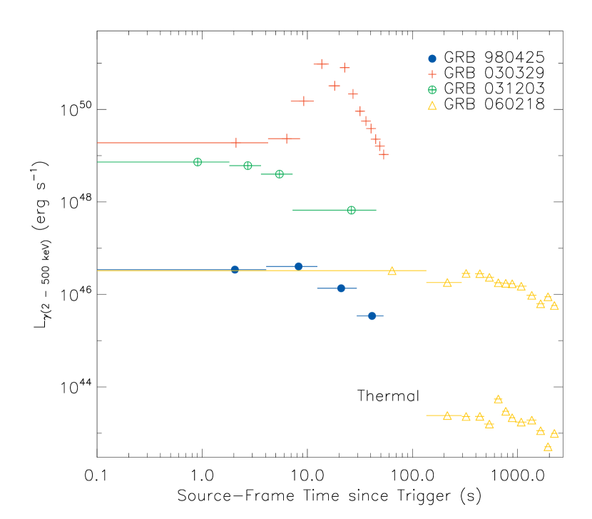
Figure 8: The evolution of the $\gamma$-ray isotropic-equivalent luminosity (2$-$500 keV, source-frame energy) for all four events, in the source-frame time. For GRB 060218, the luminosity of the thermal component is plotted separately.

The $\gamma$-ray properties of the four events are summarized in Table 4, and Figure 8 shows the evolution of their isotropic-equivalent $\gamma$-ray luminosity, $L_{\rm\gamma,iso}$ (in 2$-$500 keV, source-frame energy). For GRB 060218, the contributions from the thermal component are shown separately from the $L_{\rm\gamma,iso}$ of the non-thermal component. We find that GRB 060218 had similar $\gamma$-ray luminosity as GRB 980425; both were a few orders of magnitude fainter than the other two events. However, since GRB 060218 lasted considerably longer than GRB 980425, its $E_{\rm\gamma,iso}$ was $\sim 50$ times larger.

We should emphasize here that we measure directly only the energy radiated in the direction of the Earth per second per steradian per logarithmic energy interval by a source at luminosity distance $d_{L}$. The apparent bolometric luminosity may be quite different from the true bolometric luminosity if the source is not isotropic.

To compare the lightcurves of these events, we fitted a two-sided Gaussian function to the main pulses of the lightcurves. We found that the time profiles of these events are similar to the overall profile found for GRBs (Nemiroff et al., 1994), with the rising part having a Half Width Half Maximum (HWHM) much smaller ($<1/2$) than the HWHM of the decaying part.

2.5.1 Duration-Integrated Spectra

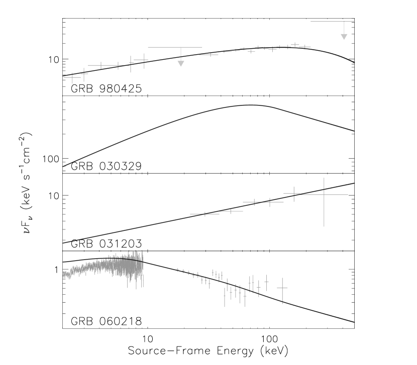
Figure 9: The unabsorbed best-fit duration-integrated spectra (solid lines) of the four events, overplotted with the deconvolved data (gray crosses) in the source-frame energy. The data are binned for display purposes. The analysis tool for the HETE-2 data of GRB 030329 was not publicaly available, and we only show here the spectral model presented in Vanderspek et al. (2004). See also text in § 2.5.1.

Figure 9 compares the best-fit duration-integrated spectra ($2-500$ keV in source frame) of the four events in $\nu F_{\nu}$, which shows the energy radiated per logarithmic photon energy interval. We plot here the unabsorbed spectral models in each case (solid lines) together with the spectrally deconvolved, blue-shifted data points shown in gray. The data are binned here for display purposes. No absorption correction was necessary in the combined LAD-WFC fit of GRB 980425. We used the published spectrum for GRB 030329, and we extrapolated our best-fit model for GRB 031203 to the lower energy range shown here. For GRB 060218 the absorption correction was significant as seen from the comparison of the model to the XRT data below 10 keV.

In Figure 10 we compare the $\nu F_{\nu}$ peak energy, ${\mathcal{E}}_{\rm peak}$, of the same duration-integrated spectra, to the ${\mathcal{E}}_{\rm peak}$ distributions of 251 bright BATSE GRBs (Kaneko et al., 2006) and 37 HETE-2 GRB/XRFs (Sakamoto et al., 2005). The ${\mathcal{E}}_{\rm peak}$ values of the four events are lower (softer) than the average value of the bright BATSE GRBs but they all seem to fit well within the HETE-2 ${\mathcal{E}}_{\rm peak}$ distribution. Note that the BATSE ${\mathcal{E}}_{\rm peak}$ distribution shown here is derived using the brightest BATSE GRBs, which tend to be spectrally harder than dim GRBs (Mallozzi et al., 1995).

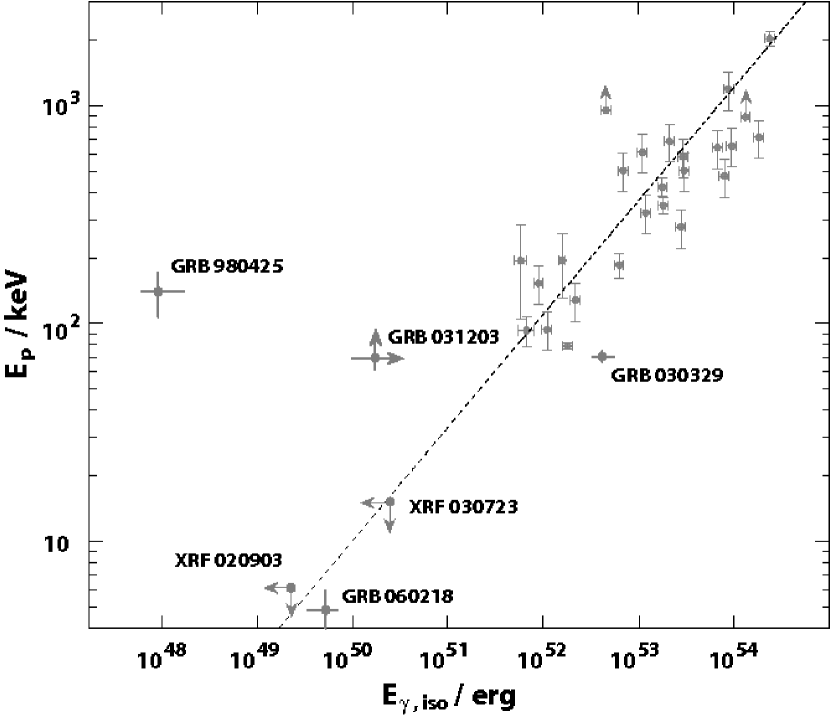
Figure 11: Locations of GRBs 980425, 031203, 030329, and 060218 in the ${\mathcal{E}}_{\rm peak}$-$E_{\rm\gamma,iso}$ plane. The dashed line indicates the correlation found by Amati et al. (2002). The events presented in Ghirlanda, Ghisellini, & Lazzati (2004) are also shown here.

Finally, in Figure 11, we show where these four events fall in the ${\mathcal{E}}_{\rm peak}$-$E_{\rm\gamma,iso}$ plane, in comparison to the empirical correlation (dashed line) found by Amati et al. (2002) and Lloyd-Ronning & Ramirez-Ruiz (2002). GRB 980425 lies farthest from the so-called Amati relation. Although GRB 031203 also lies away from the relation, this deviation could be the result of a viewing angle slightly outside the edge of the jet (Ramirez-Ruiz et al., 2005). In fact, we find a smaller lower limit on ${\mathcal{E}}_{\rm peak}$ for this event than previously reported, so it is possible that, after correcting for an off-axis viewing angle, it would be consistent with the relation (compare our Figure 11 to the left panel in Figure 3 of Ramirez-Ruiz et al., 2005). We also note that for GRBs 980425 and 031203, Ghisellini et al. (2006) have recently suggested two other possible scenarios that may cause such a deviation from the Amati relation: one is that the GRB radiation may have passed through a scattering screen, and the other is that we may have missed softer emission from the GRBs lasting much longer. In both cases, observed spectra could have much higher ${\mathcal{E}}_{\rm peak}$ values than the intrinsic ones. Altogether, the four events do not appear to follow a specific pattern or correlation in the ${\mathcal{E}}_{\rm peak}$-$E_{\rm\gamma,iso}$ plane.

2.5.2 Spectral Evolution

Figure 12 shows the hardness ratio evolution of all four events, in their source-frame time. The hardness ratio is defined here as the ratio of the energy flux between 50$-$500 keV and 2$-$50 keV in the source-frame energy. The hard-to-soft evolution is seen in all events except GRB 031203. The lack of spectral evolution in GRB 031203 is probably due to the fact that this burst was relatively dim and the observed energy range was fairly narrow. The burst was only detected below 200 keV (see Figure 4) and the break energy seemed to always lie around or above this energy; therefore, the flux above this energy may have been overestimated. We also show in Figure 13, the evolution of the ${\mathcal{E}}_{\rm peak}$ in three events (GRBs 980425, 030329, and 060218) for which the ${\mathcal{E}}_{\rm peak}$ values were determined from their time-resolved spectra. To characterize the decaying behavior, we fitted a power law (${\mathcal{E}}_{\rm peak}\propto t^{\phi}$) to each of the data sets. Since we are only interested in the decaying behavior, the first points of GRBs 980425 and 060218 were excluded from the fits. We found $\phi=-1.46\pm 0.12$, $-1.17\pm 0.08$, and $-1.40\pm 0.06$, respectively; the best-fit power laws are shown as dotted lines in Figure 13. We note that in the external shock model, for example, if ${\mathcal{E}}_{\rm peak}$ is identified with the typical synchrotron frequency $\nu_{m}$, it is expected to scale as $t^{-3/2}$ once most of the energy is transfered to the external medium and the self-similar deceleration phase sets in (Blandford & McKee, 1976). This decaying index is actually similar to what we observed here, especially when taking into account that the asymptotic power law of $t^{-3/2}$ is expected to be approached gradually rather than immediately.

3 Afterglow Emission

3.1 X-ray Afterglow

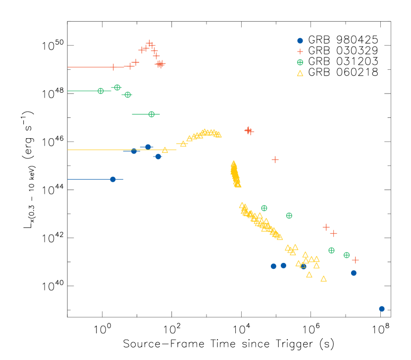
Figure 14: Evolution of the X-ray (0.3$-$10 keV, source-frame energy) prompt and afterglow luminosity (isotropic equivalent) in the source-frame time.

Figure 14 shows the evolution of the prompt and afterglow isotropic-equivalent luminosity in 0.3$-$10 keV ($L_{\rm X,iso}$) in the source-frame time for all four events. We estimated the prompt X-ray luminosity values from the spectral analysis of the prompt $\gamma$-ray emission (§2) by extrapolating the best-fit $\gamma$-ray spectra to the X-ray energy range for each event. The afterglow X-ray luminosity values were obtained in various ways.

For GRB 030329, we derived the values using the data presented in Tiengo et al. (2003, 2004). In the case of GRB 031203, we analyzed the (now) archival XMM and Chandra observations. Our analysis results are consistent with those presented in Watson et al. (2004). For GRB 060218, we analyzed the Swift XRT photon counting (PC) mode data, starting $\sim 6200\;$s after the burst trigger. We extracted two time-averaged spectra, covering 6191$-$8529 s and $1.1\times 10^{4}-1.3\times 10^{5}$ s after the burst trigger, respectively, to account for spectral evolution, and fitted each spectrum with a single power law. The spectral parameters were then used to convert the count rates to the luminosity values. The PC data after $1.3\times 10^{5}$ s were associated with relatively large uncertainties due to the fact that the count rates were approaching the XRT sensitivity limit, and therefore, we used the fitted parameters of the second spectrum above to estimate the luminosity values for these data points. We also include in this plot the two Chandra observations of GRB 060218 at $\sim 10^{6}$ s after the burst trigger, which were presented in Soderberg et al. (2006). Finally, we reanalyzed the BeppoSAX observations of GRB 980425/SN 1998bw, which were initially presented in Pian et al. (2000). We used only the data from the BeppoSAX/Medium Energy Concentrator Spectrometers and followed closely the procedure described in Pian et al. (2000). The only potentially significant differences between the current and the analysis of Pian et al. (2000) is that we estimated the background using the same observation, while Pian et al. (2000) used calibration blank-sky observations. As a result, we found slightly lower net count rates (1.6$-$10.0 keV) during the two observations in April 1998 (as compared to Table 1 in Pian et al., 2000), indicating a slightly flatter decay than was initially reported. In addition, we found that the observation beginning April 27 1998 contained $6.1\;$ks less data than previously reported (total of 14,862 s exposure time). The count rates and exposure times for the remaining observations are consistent with Pian et al. (2000).

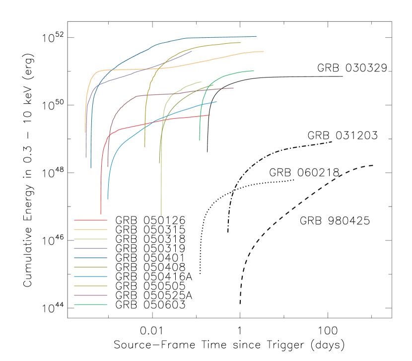
Figure 15: Cumulative total emitted energy (isotropic equivalent) of the four SN-GRBs (black lines) in 0.3$-$10 keV (source-frame energy) as a function of source-frame time. As a comparison, the cumulative energy of the 10 Swift GRBs with known redshifts published in Nousek et al. (2006) are also shown here in color.

To investigate the energy dissipation behavior in the X-ray afterglow, we fitted a natural cubic spline function to the $L_{\rm X,iso}$ history for each individual afterglow and estimated the cumulative emitted energy as a function of time. The evolution of the cumulative X-ray afterglow energy for all four events is shown in Figure 15. The integration time intervals varied from event to event, since the data time coverage was different for each event. We defined the integration time (i.e., “afterglow” time interval) of each event to be from the earliest X-ray observation time ($\sim 10^{4}$ s) to the time of the latest available data point. In the case of GRB 060218, however, it was difficult to determine the starting point of the afterglow since the prompt emission was extremely soft and long and the X-ray follow-up started much earlier than in the other three events. It is possible that the steep decay observed before $\sim 10^{4}$ s (see Figure 14) belongs to the decaying part of the prompt emission; we, therefore, chose the afterglow starting time for this event to be $1.1\times 10^{4}\;$s, which corresponds to the onset of the break in its $L_{\rm X,iso}$ history.

To compare the cumulative energy evolution to regular GRBs, we also show in Figure 15 the cumulative energy evolution of the 10 Swift GRBs with known redshifts that were presented in Nousek et al. (2006). For these 10 events, we converted the $L_{\rm X,iso}$ values in 2$-$10 keV presented there, to the $L_{\rm X,iso}$ in the energy range we used for our four events here (i.e., 0.3$-$10 keV), using the same spectral parameters used in Nousek et al. (2006), and again, fitted a spline function to each $L_{\rm X,iso}$ evolution. The start and end times of the integration were the first and the last points of the actual observations. Figure 15 shows that the final $E_{\rm X,iso}$ values for most of the 10 Nousek et al. (2006) GRBs span the range of $\sim 10^{50}-10^{52}\;$erg. Out of the four SN-GRB events, only GRB 030329 falls within this range, while the other three events fall between $\sim 10^{48}\;$ and $\sim 10^{49}\;$erg. We note that there exists a selection effect based on the observed photon flux: an event would be more likely to be detected when it is closer to us than farther, for a given intrinsic luminosity. Therefore, the difference could be partially due to the fact that these four events occured relatively nearby compared to the 10 Swift events. From the cumulative X-ray energy evolution, we also derived ${\rm T}_{\rm 90,X}$ values for all events, which we define here as the time in the source frame during which 90% of the radiated afterglow energy (0.3$-$10 keV in the source frame) is accumulated. Table 4 displays the comparison of the X-ray afterglow properties of all four events, along with their $\gamma$-ray prompt properties. Again for the purpose of comparison, Figure 16 shows the $E_{\rm\gamma,iso}$, $E_{\rm X,iso}$, and ${\rm T}_{\rm 90,X}$ values of the four SN-GRBs, along with those of the 10 Nousek et al. (2006) GRBs. Here we plot the $E_{\rm\gamma,iso}$ values between 20$-$2000 keV (in the source frame). There is a clear correlation between $E_{\rm\gamma,iso}$ and $E_{\rm X,iso}$ ($E_{\rm\gamma,iso}\propto E_{\rm X,iso}^{1.0\pm 0.3}$), and an anti-correlation between $E_{\rm\gamma,iso}$ and ${\rm T}_{\rm 90,X}$ ($E_{\rm\gamma,iso}\propto{\rm T}_{\rm 90,X}^{-1.2\pm 0.3}$). We also find ${\rm T}_{\rm 90,X}\propto E_{\rm X,iso}^{-0.7\pm 0.2}$, which can be interpreted as follows.

Events that have large isotropic-equivalent energy (both in $\gamma$-rays, $E_{\rm\gamma,iso}$, and in the kinetic energy of their afterglow, $E_{\rm k,iso}$) have a large $E_{\rm X,iso}$, indicating a reasonably narrow spread in the efficiency of converting the afterglow kinetic energy into radiation. Moreover, they are typically associated with narrow jets. This means that most of their kinetic energy is in relativistic outflow carried by highly-relativistic ejecta (with $\Gamma\sim 30-50$; Granot & Kumar, 2006). Therefore, they have a relatively small ${\rm T}_{\rm 90,X}$; the time at which most of the energy is injected into the afterglow shock, of the order of $10^{3}\;{\rm s}\lesssim t_{\rm break,2}\lesssim 10^{4}\;$s (Nousek et al., 2006). On the other hand, events that have a small $E_{\rm k,iso}$ and small $E_{\rm\gamma,iso}$, naturally have a small $E_{\rm X,iso}$. Such events also tend to have most of their relativistic outflow energy residing in mildly relativistic ejecta, rather than in highly relativistic ejecta (Granot & Ramirez-Ruiz, 2004; Waxman, 2004). As a result, most of the kinetic energy is transfered to the afterglow shock at relatively late times, hence a large ${\rm T}_{\rm 90,X}$. Further, since such events tend to be only mildly collimated, the true total energy in relativistic ($\Gamma\gtrsim 2$) ejecta has a significantly smaller spread than the one of the isotropic equivalent energy ($E_{\rm\gamma,iso}$ or $E_{\rm X,iso}$).

3.2 Radio Afterglow

We performed radio observations of GRB 060218 with the Westerbork Synthesis Radio Telescope (WSRT); these results are tabulated in Table 5. Additional radio data for this burst and radio data for the three other events were collected from the literature (GRB 980425; Frail et al. 2003 and Kulkarni et al. 1998, GRB 030329; Berger et al. 2003, Frail et al. 2005, Taylor et al. 2005, van der Horst et al. 2005, and Resmi et al. 2005, GRB 031203; Soderberg et al. 2004, GRB 060218; Soderberg et al. 2006 and Kamble et al. 2006). The radio flux lightcurves in 4.8/4.9 GHz, at which all of the four events were observed, are shown in Figure 17.

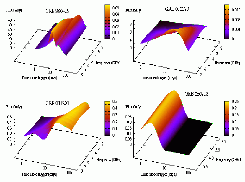
Figure 18: Spline fits to the broadband radio lightcurves for the four events.

As with the X-ray afterglow, we fitted the flux lightcurve of each event (in a wide band, where available) with a natural cubic spline, to estimate the cumulative energy evolution emitted in radio. To minimize the effect of scintillation in the radio lightcurves, we used fewer nodes than data points in the fitting. This resulted in a smooth fit to the data that retains the overall evolution of the lightcurve. The curve is forced to be 0 at very early times ($<0.01\;$days) and late times ($>500\;$days), or to the inferred flux of the host galaxy in the case of GRB 031203 (Soderberg et al., 2004). The fitted lightcurves were then used to create a grid in time-frequency space to obtain the flux profile in a wider frequency range (Figure 18). Using this, we constructed the cumulative radio afterglow energy evolution in 5$-$7 GHz, shown in Figure 19. In Table 4, we also present the comparison of the radio afterglow properties of the four events, along with their $\gamma$-ray prompt and X-ray afterglow properties. Similar to ${\rm T}_{\rm 90,X}$ defined above, we define ${\rm T}_{\rm 90,R}$ here as the time in the source frame during which 90% of the radiated afterglow energy is accumulated in 5$-$7 GHz in the source-frame energy. The integration time of the radio afterglow emission is 1 day to 100 days after the burst trigger time, in the rest frame of the source.

As can be seen in Table 4, the isotropic equivalent energy that is radiated in the radio ($E_{\rm R,iso}$) is $\sim 3.5-5$ orders of magnitude smaller than that in X-rays, $E_{\rm X,iso}$. This is predominantly due to the fact that $\nu F_{\nu}$ typically peaks closer to the X-rays than to the radio, and it is very flat above its peak while it falls much faster toward lower energies. Another effect that enhances the difference between $E_{\rm R,iso}$ and $E_{\rm X,iso}$ is that the latter is calculated over a much wider energy range ($0.3-10\;$keV versus $5-7\;$GHz). Finally, since these are isotropic equivalent energies, most of the contribution to $E_{\rm R,iso}$ is from significantly later times than for $E_{\rm X,iso}$, and the collimation of the outflow together with relativistic beaming effects could result in much larger $E_{\rm X,iso}$ than $E_{\rm R,iso}$. We note that for at least two (GRB 908425 and GRB 060218) of the SN-GRBs, the isotropic-equivalent emitted energy at optical wavelengths can be (much) larger than $E_{\rm X,iso}$ because it is typically dominated by the contribution from the SNe (powered by radioactive decay) rather than by the GRB afterglow emission (see also § 5).

4 Prompt and Afterglow Properties

The isotropic-equivalent luminosity of GRB X-ray afterglows scaled to $t=10$ hr after the burst in the source frame, $L_{\rm X,iso}$(10 hr), can be used as an approximate estimator for the energy in the afterglow shock for the following reasons. First, at $10\;$hr the X-ray band is typically above the two characteristic synchrotron frequencies, $\nu_{m}$ (of the accelerated electron with minimum energy) and $\nu_{c}$ (of the electron whose radiative cooling time equals the dynamical time), so that the flux has very weak dependence on $\epsilon_{B}$ and no dependence on the external density, both of which are associated with relatively large uncertainties. Second, at $10\;$hr the Lorentz factor of the afterglow shock is sufficiently small ($\Gamma\sim 10$) so that a large fraction of the jet is visible (out to an angle of $\sim\Gamma^{-1}\sim 0.1\;$rad around the line of sight) and local inhomogeneities on small angular scales are averaged out. Finally, the fact that the ratio of $L_{\rm X,iso}$(10 hr) and $E_{\rm\gamma,iso}$ is fairly constant for most GRBs, suggests that both can serve as a reasonable measure of the isotropic-equivalent energy content of the ejected outflow.

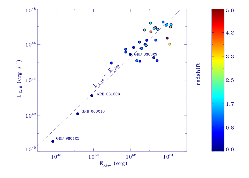
Figure 20: Isotropic-equivalent luminosity of SN-GRB X-ray afterglows scaled to t = 10 hr (source frame; 2$-$10 keV) after the burst trigger as a function of their isotropic $\gamma$-ray energy release (20$-$2000 keV). The redshift for each event is also shown in color (adopted from Nousek et al., 2006).

Figure 20 shows $L_{\rm X,iso}$(10 hr) in 2$-$10 keV rest-frame energy as a function of their isotropic $\gamma$-ray energy release ($E_{\rm\gamma,iso}$, in 20$-$2000 keV) for the four events, in comparison to regular GRBs. A linear relation, $L_{\rm X,iso}(10\,{\rm hr})\propto E_{\rm\gamma,iso}$, seems to be broadly consistent with the data, probably suggesting a roughly universal efficiency for converting kinetic energy into gamma rays in the prompt emission for these four events and those of “regular” long GRBs. This “universal” efficiency is also likely to be high (i.e., the remaining kinetic energy is comparable to, or even smaller than, the energy dissipated and radiated in the prompt emission). If this is the case, the well-known efficiency problem for long GRBs also persists for SN-GRB events. Not surprisingly, there is also a correlation between the cumulative X-ray afterglow energy and isotropic $\gamma$-ray energy (see Figure 16 and also § 6).

5 SN Properties

Pian et al. (2006) presented the bolometric luminosity evolution (in optical and near-infrared wavelengths; 3000$-$24000 Å) for all the SNe associated with the GRBs considered here, namely SNe 1998bw, 2003dh, 2003lw, and 2006aj. We fitted a cubic spline to the luminosity evolution of each SN (Figure 3 of Pian et al., 2006), and estimated the cumulative energy emitted by the SN as a function of source-frame time. To prevent the spline fits to diverge after the last real data points ($\leq$ 40 days), we assumed that the luminosity becomes much smaller ($\ll 10^{41}\;$erg s^-1) at much later time ($\gg 1000\;$days). The cumulative SN energy history is plotted in Figure 21 for all four SNe. We also estimated ${\rm T}_{\rm 90,SN}$, during which 90% of the SN energy is accumulated in 3000$-$24000 Å since 1 day after the burst, as well as the total energy emitted in the same energy range, $E_{\rm SN,iso}$. These values are presented in Table 4, along with the burst properties in other wavelengths. It should be noted here that in most cases, $E_{\rm SN,iso}$ is monopolized by the SN emission while the GRB afterglow dominates at all other wavelengths. The integration time for the SN cumulative energy was from 1 day to 100 days after the burst trigger. The cumulative energy of the four SNe span a much narrower range than the one reported for the entire SNe Ic class (Mazzali et al., 2006a). Among these four, SN 2006aj is the least energetic, albeit more energetic than other broad-lined SNe and normal SNe (Pian et al., 2006).

Furthermore, from the radio observations of type Ib/c SNe presented by Weiler et al. (2002), we note that the peak radio luminosity of SN 1998bw observed at 6 cm (5 GHz) was a few orders of magnitude higher than the other type Ib/c SNe, although the overall time evolution of this event was comparable to the others.

6 Discussion

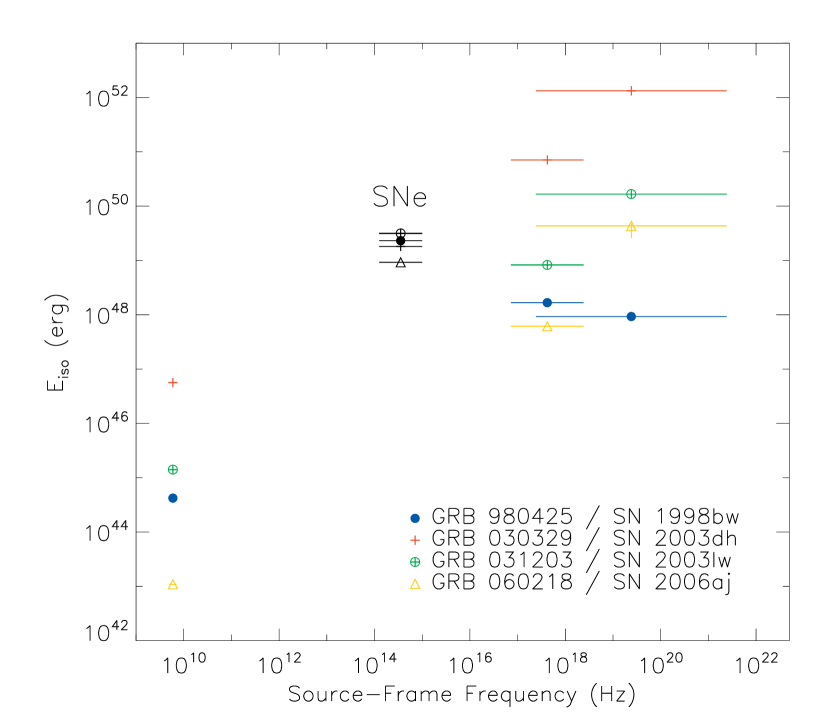
Figure 22: Summary of the isotropic-equivalent total emitted energy of the prompt and afterglow emission of the four GRBs, along with the properties of their associated SNe. The energetics in $\gamma$-ray, X-ray, Radio, and Optical (for SNe) wavelengths correspond to 1$-$10,000 keV, 0.3$-$10 keV, 5$-$7 GHz, 3000$-$24000 Å in the source frame, respectively.

The compilation of the radiated energy inventory, presented in Table 4 and Figure 22, offers an overview of the integrated effects of the energy transfers involved in all the physical processes of long GRB evolution, operating on scales ranging from AU to parsec lengths. The compilation also offers a way to assess how well we understand the physics of GRBs, by the degree of consistency among related entries. We present here our choices for the energy transfers responsible for the various entries in the inventory. Many of the arguments in this exercise are updated versions of what is in the literature, but the present contribution is the considerable range of consistency checks, which demonstrates that many of the entries in the inventory are meaningful and believable.

In the following, § 6.1 repeats the minimal Lorentz factor estimates in Lithwick & Sari (2001) using the parameters inferred for all of the four SN-GRB events in this work. § 6.2 compares a simple model for the emitted radiation to the observational constraints on the integrated energy radiated in the afterglow phase. Finally, the energy contents in relativistic and sub-relativistic form are estimated in §§ 6.3 and 6.4, respectively.

6.1 Constraints on the Lorentz Factor

As is well known, the requirement that GRBs are optically thin to high-energy photons yields a lower limit on the Lorentz factor of the expansion. We estimate here the minimal Lorentz factor of the outflow based on our observational analysis, by using the results of Lithwick & Sari (2001). They derived two limits; A and B. Limit A is from the requirement that the optical depth to pair production in the source for the photon with the highest observed energy, $\mathcal{E}_{\rm max}$, should be smaller than unity. Limit B is from the requirement that the Thompson optical depth of the $e^{\pm}$ pairs that are produced by the high-energy photons in the source does not exceed unity. The required parameters to estimate these limits are the variability time of the $\gamma$-ray lightcurve, $\delta T$ (which is related to the radius of emission by $R\sim\Gamma^{2}c\delta T$), and the photon flux per unit energy, $dN_{\rm ph}/dAdtd\mathcal{E}_{\rm ph}=f\mathcal{E}_{\rm ph}^{-\beta}$ for $\mathcal{E}_{\rm min}<\mathcal{E}_{\rm ph}<\mathcal{E}_{\rm max}$: in the latter, both the normalization $f$ and the high energy photon index $\beta$ are needed. Although the result depends on the exact choice of parameters, representative values are presented in Table 6. For each event, we determined $\delta T$ to be the Full Width Half Maximum (FWHM) of a two-sided Gaussian function fitted to the prompt $\gamma$-ray lightcurve, the peak of which aligns with the main peak of the lightcurve. We then analyzed the “peak” spectrum with the integration time of $\delta T$ to obtain the high-energy photon index $\beta$ and the ${\mathcal{E}}_{\rm peak}$ values shown here. The minimal values of the Lorentz factor derived in this way are generally smaller for less energetic events (in terms of $E_{\rm\gamma,iso}$ or $E_{\rm X,iso}$). For the event with the smallest $E_{\rm\gamma,iso}$, GRB 980425, we find $\Gamma_{\rm min}\sim 2.4$ if we adopt our lower limit for the high-energy photon index ($\beta>3.5$; 1$\sigma$), while a larger value of $\beta$ would lower $\Gamma_{\rm min}$ (consistent with the results of Lithwick & Sari, 2001).

6.2 Integrated Radiated Energy

The integrated (isotropic-equivalent) radiated energy during the afterglow, is given by

$$E_{\rm rad,iso} = \int dt\int d\nu\,L_{\rm\nu,iso}(t)$$ (1)

$$= \eta_{t}t_{\rm peak}L_{\rm iso}(t_{\rm peak})=\eta_{t}\eta_{\nu}t_{\rm peak}\nu_{\rm peak}(t_{\rm peak})L_{\rm\nu,iso}(t_{\rm peak})\ ,$$

where $t$, $\nu$, and $L_{\rm\nu,iso}$ are measured in the cosmological frame of the GRB, $t_{\rm peak}$ is the time when $tL_{\rm iso}(t)$ peaks, $\nu$ is the frequency where $\nu L_{\rm\nu,iso}(t_{\rm peak})$ peaks;

$$\eta_{t}={\int dt\,L_{\rm iso}(t)\over t_{\rm peak}L_{\rm iso}(t_{\rm peak})}\ ,$$ (2)

and

$$\eta_{\nu}={L_{\rm iso}(t_{\rm peak})\over\nu_{\rm peak}(t_{\rm peak})L_{\rm\nu,iso}(t_{\rm peak})}\ ,$$ (3)

are factors of order unity here (although we typically expect $\eta_{t}\eta_{\nu}\sim 10$). Since in practice $\nu L_{\rm\nu,iso}$ peaks near the X-ray band, we can assume that $L_{\rm X,iso}$ only mildly underestimates $L_{\rm iso}$, and the time $t_{\rm peak}$ when $tL_{\rm iso}(t)$ peaks is usually rather close to the time $t_{\rm X}$ when $tL_{\rm X,iso}(t)$ peaks. Therefore, $t_{\rm X}L_{\rm X,iso}(t_{\rm X})$ provides a convenient lower limit for $E_{\rm rad,iso}$ within an order of magnitude, although it is still possible that the X-ray observations might have missed the actual time when most of the energy was radiated, resulting in a significant underestimate. The values of $t_{\rm X}L_{\rm X,iso}(t_{\rm X})$ are provided in Table 7. We find that these values are typically a factor of $\sim 2-3$ smaller than $E_{\rm X,iso}$, suggesting $\eta_{t}\sim 2-3$. Although $\eta_{t}$ is defined for the bolometric luminosity rather than for the X-ray luminosity, the values derived here are still fairly representative.

6.3 Energy Inventory - Relativistic Form

Supernova remnants are understood reasonably well, despite continuing uncertainty about the initiating explosion; likewise, we hope to understand the afterglow of GRBs, despite the uncertainties about their trigger mechanism. The simplest hypothesis is that the afterglow is due to a relativistic expanding blast wave. The complex time structure of some bursts suggests that the central trigger may continue (i.e., the central engine may remain active) for up to $\sim 100$ seconds. However, at much later times all memory of the initial time structure would be lost. All that matters then is essentially how much energy has been injected and its distribution in angle and in Lorentz factor, $\epsilon(>\Gamma,\theta)$, where $\epsilon\equiv dE/d\Omega$.

6.3.1 Kinetic Energy Content

An accurate estimate of the kinetic energy in the afterglow shock requires detailed afterglow modeling and good broadband monitoring, which enables one to determine the values of the shock microphysical parameters (electron and magnetic energy equipartition fractions, $\epsilon_{e}$ and $\epsilon_{B}$, and shock-accelerated electron power-law index, $p$). However, even then, it provides only a lower limit for the kinetic energy due to the conventional and highly uncertain assumption that all of the electrons are accelerated to relativistic energies (Eichler & Waxman, 2005; Granot, Königl & Piran, 2006). Nevertheless, an approximate lower limit on the isotropic-equivalent kinetic energy in the afterglow shock, $E_{\rm k,iso}$, can be obtained from the isotropic-equivalent X-ray luminosity, $L_{\rm X,iso}$, since the typical efficiency of the X-ray afterglow, $\epsilon_{\rm X}\equiv tL_{\rm X,iso}(t)/E_{\rm k,iso}(t)$, is $\lesssim 10^{-2}$ (Granot, Königl & Piran, 2006): a rough lower limit on $E_{\rm k,iso}$ is obtained by adopting $\epsilon(t_{\rm X})\sim 10^{-2}$, where $t_{\rm X}$ is defined in the previous section and the values for the four events are presented in Table 7. For GRBs 980425 and 060218, we estimate $E_{\rm k,iso}(t_{\rm X})\approx 6\times 10^{49}\epsilon_{\rm X,-2}^{-1}\;$erg, and $E_{\rm k,iso}(t_{\rm X})\approx 3\times 10^{49}\epsilon_{\rm X,-2}^{-1}\;$erg, respectively, where $\epsilon_{\rm X,-2}=\epsilon_{\rm X}(t_{\rm X})/10^{-2}$. These rough estimates are similar to the energy inferred from a more detailed analysis of the X-ray and radio observations of this event ($E_{\rm k,iso}\approx 5\times 10^{49}\;$erg; Waxman, 2004). For GRB 031203, we find $E_{\rm k,iso}(t_{\rm X})\approx 2\times 10^{50}\epsilon_{\rm X,-2}^{-1}\;$erg.

For GRB 030329, we derive $E_{\rm k,iso}(t_{\rm X})\approx 5\times 10^{52}\epsilon_{\rm X,-2}^{-1}\;$erg. This estimate is comparable to that from the broadband spectrum at $t\approx 10\;$days ($E_{\rm k,iso}\sim 5\times 10^{52}\;$erg for a uniform density and $\sim 10^{52}\;$erg for a wind; Granot, Ramirez-Ruiz & Loeb, 2005), assuming negligible lateral expansion of the jet (Gorosabel et al., 2006). For rapid lateral expansion, the inferred value of $E_{\rm k,iso}(10\;{\rm days})$ is lower ($\sim 1.6\times 10^{51}-5\times 10^{51}\;$erg, Berger et al., 2003; Granot, Ramirez-Ruiz & Loeb, 2005) but should correspond to a similar $E_{\rm k,iso}$ before the jet break time ($t_{j}\approx 0.5\;$days), for a comparable initial half-opening angle. There were, however, several re-brightening episodes observed in the optical afterglow lightcurve of GRB 030329, between $\sim 1.5\;$days and a week after the GRB (Lipkin et al., 2004), suggesting energy injection into the afterglow shock that increased its energy by a factor of $\sim 10$ (Granot, Nakar & Piran, 2003). This would imply that $E_{\rm k,iso}$ at $t_{\rm X}\approx 2\times 10^{4}\;$s was a factor of $\sim 10$ lower than our rough estimate, or that $\epsilon_{\rm X}(t_{\rm X})$ is as high as $\sim 0.1$. A possible alternative explanation for the relatively high value of $t_{\rm X}L_{\rm X,iso}(t_{\rm X})$ which does not require a high afterglow efficiency ($\epsilon_{\rm X}$) comes about if a flare in the X-rays was present around $t_{\rm X}$, which was not detected in the optical lightcurve at the similar time. In this case, $L_{\rm X,iso}(t_{\rm X})$ would be dominated by late time activity of the central source rather than by emission from the external shock (Ramirez-Ruiz et al., 2001; Granot, Nakar & Piran, 2003).

6.3.2 Minimal Energy Estimates

Here we derive a simple but rather robust estimate for the minimal combined energy in the magnetic field ($E_{B}$) and in the relativistic electrons ($E_{e}$) that are responsible for the observed synchrotron emission of flux density $F_{\nu,R}$ at some frequency $\nu_{R}$, $E_{\rm min}=\min(E_{B}+E_{e})$. This estimate is applied for the sub-relativistic flow, to avoid the effects of relativistic beaming and reduce the uncertainty on the geometry of the emitting region. Since the source is not resolved, the energy is estimated near the time of the non-relativistic transition, $t_{\rm NR}$, where we have a handle on the source size.

We follow standard equipartition arguments (Pacholczyk, 1970; Scott & Readhead, 1977; Gaensler et al., 2005; Nakar, Piran & Sari, 2005). The minimal energy is obtained close to equipartition, when $E_{B}/E_{e}=3/4$. At such late times ($t\sim t_{\rm NR}\gtrsim 10^{2}\;$days) it is easiest to detect the afterglow emission in the radio, so $\nu_{R}$ would typically be in the radio band. Furthermore, $\nu_{m}(t_{\rm NR})$ is also usually around the radio band, meaning that the electrons radiating in the radio would carry a reasonable fraction of the total energy in relativistic electrons. Still, the total energy of all electrons would be a factor of $\gtrsim 10$ larger than $E_{e}$, which would increase the total minimal energy by a factor of $\gtrsim 6$. Since the kinetic energy is expected to be at least comparable to that in the relativistic electrons and in the magnetic field, the total energy is likely to be at least an order of magnitude larger than $E_{\rm min}$.

Following Nakar, Piran & Sari (2005), $E_{e}=N_{e}\gamma_{e}m_{e}c^{2}$, where $N_{e}$ is the number of electrons with a synchrotron frequency $\nu_{\rm syn}\sim\nu_{R}$, and therefore, with a Lorentz factor $\gamma_{e}\approx[2\pi m_{e}c(1+z)\nu_{R}/eB]^{1/2}$. Also, since $F_{\nu,R}\approx N_{e}P_{\nu,{\rm max}}(1+z)/4\pi d_{L}^{2}$ where $P_{\nu,{\rm max}}\approx P_{\rm syn}(\gamma_{e})/\nu_{\rm syn}(\gamma_{e})\approx\sigma_{T}m_{e}c^{2}B/3e$, $N_{e}\approx 12\pi d_{L}^{2}eF_{\nu,R}/(1+z)\sigma_{T}m_{e}c^{2}B$. Estimating the emitting volume as $V=(4\pi/3)R^{3}/\eta$ with $\eta=10\eta_{1}$ ($\eta^{-1}$ is the fraction of the volume of a sphere with the radius $R$ of the emitting material that is actually occupied by the emitting material), while in terms of our observed quantity, $t_{\rm NR}$, $R(t_{\rm NR})=act_{\rm NR}/(1+z)$ with $a=2a_{0.3}$ ($a$ is the average apparent expansion velocity at $t_{\rm NR}$ in the cosmological frame of the GRB/SN in units of the speed of light), we obtain

$$E_{\rm min}=6\times 10^{49}a_{0.3}^{9/7}\eta_{1}^{-3/7}(1+z)^{-19/14}d_{L28}^{8/7}\left(\frac{F_{\nu,R}}{1\;{\rm mJy}}\right)^{4/7}\left(\frac{\nu_{R}}{5\;{\rm GHz}}\right)^{2/7}\left(\frac{t_{\rm NR}}{100\;{\rm days}}\right)^{9/7}\ {\rm ergs}.$$ (4)

The resulting estimates of $E_{\rm min}$ for the four events discussed in this paper are given in Table 8, along with $t_{\rm NR}$, and $F_{\nu,R}$ values. We used $\nu_{R}=4.86$ GHz. As a sanity check, we calculate the minimal external density that corresponds to a total energy of $10E_{\rm min}$; $n_{\rm min}=10E_{\rm min}/(4\pi/3)R_{\rm NR}^{3}m_{p}c^{2}$, where $R_{\rm NR}=R(t_{\rm NR})=act_{\rm NR}/(1+z)$, in which we use our fiducial values of $a=2$ and $\eta=10$. These values are also presented in Table 8. It is useful to compare $E_{\rm min}$ to other energy estimates. For GRB 980425, the X-ray afterglow observations suggest an energy of $\sim 5\times 10^{49}\;$erg $\sim 30E_{\rm min}$ in a mildly relativistic roughly spherical component (Waxman, 2004). For GRB 030329 the total kinetic energy at late times is estimated to be $\sim 3.2\times 10^{50}\;$erg $\sim 100E_{\rm min}$ (Granot, Ramirez-Ruiz & Loeb, 2005). Therefore, it can be seen that while the ratio of the total kinetic energy in relativistic outflow ($\gamma\beta>1$) around $t_{\rm NR}$ and $E_{\rm min}$ is indeed $\gtrsim 10$, it is typically $\lesssim 100$. Moreover, the fact that these different energy estimates are consistent lends some credence to these models.

Some cautionary remarks are in order. The above calculation is only sketchy and should be taken as an order of magnitude estimate at present. For example, the usual assumption that at $t_{\rm NR}$ the flow is already reasonably well described by the Newtonian spherical Sedov-Taylor self-similar solution, for which $\eta\approx 10$, is probably not a very good approximation. Numerical studies show that there is very little lateral expansion of the GRB jets while the flow is relativistic, and therefore it takes at least several dynamical timescales after $t_{\rm NR}$ for the flow to approach spherical symmetry. Furthermore, since the flow is still mildly relativistic at this stage, there is still non-negligible relativistic beaming of the radiation toward the observer from the forward jet and away from the observer from the counter-jet. Altogether, the flux is somewhat enhanced due to this mild beaming, and the fraction of the total solid angle that is occupied by the flow at $t_{\rm NR}$ is still considerably smaller than unity. Consequently, this introduces an uncertainty of at least a factor of a few in the estimate of $E_{\rm min}$; however, since the total energy is expected to be $\gtrsim 10E_{\rm min}$, it would still be at least a factor of a few larger than our estimate of $E_{\rm min}$. The theoretical uncertainty on the dynamics of the flow should improve with time as more detailed numerical studies become available.

Another important uncertainty is in the determination of the non-relativistic transition time, $t_{\rm NR}$. The better estimate of $E_{\rm min}$ should become obtainable as more well-sampled afterglow observations are made, and the modeling gets more precise so that one can more carefully estimate both $t_{\rm NR}$ and $F_{\nu,R}(t_{\rm NR})$. For GRB 980425 we related $t_{\rm NR}$ to the time at which the X-ray lightcurve steepens, which likely corresponds to the deceleration time of the mildly relativistic ejecta. For GRB 030329, $t_{\rm NR}$ was selected to roughly correspond to the time at which the radio lightcurve flattens and at the same time to be consistent with estimates derived from direct size measurements of the event (Oren, Nakar & Piran, 2004; Granot, Ramirez-Ruiz & Loeb, 2005). In the other two cases, only a crude estimate of $t_{\rm NR}$ can be made as it is unclear whether current observations clearly display a signature of the non-relativistic transition.

6.4 Energy Inventory - Sub-relativistic Form

Despite the wide range in energies in relativistic ejecta, and even wider range in $E_{\rm\gamma,iso}$, the total (non-neutrino) energy of the associated SN in all four events spans, at most, a factor of 10. Most of this energy is in non-relativistic ($\gamma\beta<2$) kinetic energy: the integrated light of the SN is negligible. While not standard candles, the optical luminosities of the four SNe at peak are all much brighter than average Type Ib or Ic SNe (Woosley & Bloom, 2006; Pian et al., 2006; Ferrero et al., 2006). Since the brightness of Type I supernovae at peak is given by the instantaneous rate of decay of ⁵⁶Ni, the ⁵⁶Ni masses are thus inferred to be in the range of $\sim(0.2-0.7)M_{\odot}$.

To produce this much ⁵⁶Ni in a Wolf-Rayet (WR) star requires a kinetic energy of at least $\sim 2\times 10^{51}$ erg, even in lower mass WR stars (Ensman & Woosley, 1988). In higher mass stars, a still greater energy is required for the lightcurve to peak within two weeks after the maximum. Large kinetic energies are also inferred from detailed models of the explosion, especially the lightcurve and the velocity histories of spectral features (see Woosley & Bloom, 2006, and references therein). In summary, the supernova kinetic energies in the four well-studied events almost certainly lie within the range $2\times 10^{51}-2\times 10^{52}$ erg. In fact, the range of typical GRB-SNe may be much smaller, with the brightness at peak varying by no more than one magnitude in all four events and the kinetic energy in at least three of the four events (all but SN 2006aj) within a factor of two of $1.5\times 10^{52}$ erg (Woosley & Bloom, 2006).

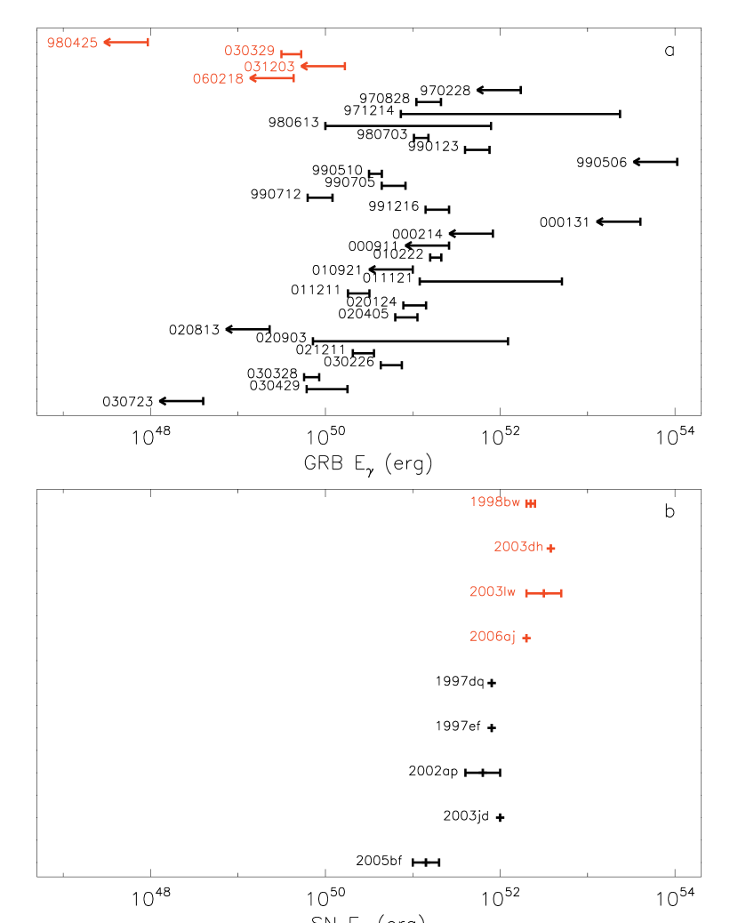
Figure 23: Comparisons of collimation-corrected total emitted $\gamma$-ray energy ($E_{\gamma}$) of the four SN-GRBs (red) and other GRBs (a), and of the SN kinetic energy ($E_{\rm k}$) of the four GRB-SNe (red) and other SNe of the same type (b). In (a), $E_{\rm\gamma,iso}$ was used as an upper limit for GRBs with no jet angle constraints.

Finally, in Figure 23, we compare the collimation-corrected total emitted energy in $\gamma$-ray ($E_{\gamma}$) and supernova kinetic energy estimates ($E_{\rm k}$) of these four SN-GRB events with regular GRBs and other broad-lined (1998-bw like) SNe without GRBs. For GRB 030329, we used the jet angle estimate of $\theta_{j}\sim 0.083-0.14\;$rad (Gorosabel et al., 2006). For the other three events, the isotropic-equivalent emitted energy, $E_{\rm\gamma,iso}$, was used as an upper limit, as there was no observational evidence of jet breaks for these events. The $E_{\gamma}$ values for 27 regular GRBs were adopted from Ghirlanda, Ghisellini, & Lazzati (2004), where the $E_{\rm\gamma,iso}$ was again used as an upper limit for GRBs with no $\theta_{j}$ constraints. All the $E_{\rm k}$ estimates were taken from the literature (SN 1998bw; Woosley, Eastman, & Schmidt 1999, SN 2003dh; Mazzali et al. 2003, SN 2003lw; Deng et al. 2005, SN 2006aj; Mazzali et al. 2006b, SN 2002ap; Mazzali et al. 2002, SN 2003jd; Mazzali et al. 2005, SN 1997dq & SN 1997dq; Mazzali et al. 2004, and SN 2005bf; Tominaga et al. 2005; Folatelli et al. 2006). We note that the explosion energy (i.e., SN $E_{\rm k}$) is much larger than the energy released as GRBs ($E_{\gamma}$), and spans much narrower range than $E_{\gamma}$.

7 Concluding Remarks

One of the liveliest debated issues associated with GRBs is on the total energy released during the burster explosion: are GRBs standard candles? The GRB community has vacillated between initial claims that the GRB intrinsic luminosity distribution was very narrow (Horack et al., 1994), to discounting all standard candle claims, to accepting a standard total GRB energy of $\sim 10^{51}$ ergs (Frail et al., 2001), and to diversifying GRBs into “normal” and “sub-energetic” classes. The important new development is that we now have significant observational support for the existence of a sub-energetic population based on the different amounts of relativistic energy released during the initial explosion. A network of theoretical tests lends credence to this idea. The existence of a wide range of intrinsic energies that we presented in this work may pose challenges to using GRBs as standard candles – it is also worth stating explicitly that, when viewed together, these four events fall away from the Amati relation.

Our results are consistent with the emerging hypothesis that GRBs and XRFs share a common origin in massive WR stars. The central engine gives rise to a polar outflow with two components (Woosley & Bloom, 2006). One large angle outflow (the SN), containing most of the energy and mass, is responsible for exploding the star and producing the ⁵⁶Ni to make the SN bright. Only a tiny fraction of the material in this component reaches mildly relativistic velocities, which is more narrowly focused. A second outflow component (the GRB jet) occupies a narrower solid angle, probably contains smaller energy (which can range from comparable to much smaller), and most of its energy is in material with relativistic velocities (where the typical Lorentz factor of the material that carries most of the energy in this component can vary significantly between different SN-GRBs). After it exits the star, internal shocks within this jet and external shocks with the residual wind material around the star make the GRB or XRF and its afterglow. Apparently, the properties of the broad component are not nearly so diverse as those of the core jet (Ramirez-Ruiz & Madau, 2004; Soderberg et al., 2006; Woosley & Bloom, 2006).

We have argued, using well-known arguments connected with parameters such as opacity and variability timescales, that these less-energetic events do not require a highly-relativistic outflow. Our best estimates of Lorentz factors, $\Gamma$, for these events are in the range of 2$-$10. Indeed, it is much more difficult to produce a jet with very high Lorentz factor – i.e., a high energy loading per baryon – than with low Lorentz factor. A jet with low Lorentz factor could result even if a jet of relatively pure energy is produced, since it may be loaded with excess baryons by instabilities at its walls as it passes through the star, or if it does not precisely maintain its orientation (Ramirez-Ruiz, Celotti & Rees, 2002; Aloy et al., 2002; Zhang, Woosley & Heger, 2004). The above suggest that GRBs made by jets with lower Lorentz factor should be quite common in the universe (Granot & Ramirez-Ruiz, 2004).

Continued advances in the observations will surely yield unexpected revisions and additions in our understanding of GRBs in connection with SNe: currently, we are attempting to draw large conclusions from limited observations of exceedingly complex phenomena. However, the big surprise at the moment is that these SN-GRB events appear to be intrinsically different from and much more frequent (Granot & Ramirez-Ruiz, 2004; Guetta et al., 2004; Pian et al., 2006) than luminous GRBs, which have been observed in large numbers out to higher redshifts.

We are very grateful to Scott Barthelmy and Takanori Sakamoto for their help with the Swift BAT data analysis, to Rob Preece and Michael Briggs for their help with the BATSE-WFC joint analysis, and to Ersin Göğüş for helpful discussions. We also thank the WSRT staff, in particular Tony Foley. This work is supported by IAS and NASA under contracts G05-6056Z (YK) and through a Chandra Postdoctoral Fellowship award PF3-40028 (ERR), by the Department of Energy under contract DE-AC03-76SF00515 (JG), and by PPARC (ER). SEW acknowledges support from NASA (NNG05GG08G), and the DOE Program for Scientific Discovery through Advanced Computing (SciDAC; DE-FC02-01ER41176). RAMJW is supported by the Netherlands Foundation for Scientific Research (NWO) through grant 639.043.302. This paper benefited from collaboration through an EU-funded RTN, grant number HPRN-CT-2002-00294. The Westerbork Synthesis Radio Telescope is operated by ASTRON (Netherlands Foundation for Research in Astronomy) with support from NWO.

Figure 1: Lightcurves of GRB 980425 detected with the brightest BATSE LAD (20$-$2000 keV; top) and with the BeppoSAX WFC (2$-$27 keV; bottom) plotted with 1-s resolution. The four time intervals used in the current analysis are labeled with A, B, C, and D. The dotted lines indicate background levels.

Figure 2: Spectral parameter evolution of GRB 980425; the data points correspond to the intervals indicated in Figure 1. The uncertainties are 1$\sigma$.

Figure 3: The HETE-2/FREGATE lightcurve of GRB 030329 generated using the publicly available Burst Lightcurve data integrated in 64-ms resolution time bins.

Figure 4: The INTEGRAL IBIS/ISGRI lightcurve of GRB 031203 in 1-s resolution. The four time intervals used in the current analysis are indicated with the dashed lines. The dotted lines show the background levels.

Figure 5: Single power law spectral index evolution of GRB 031203; the data points correspond to the intervals indicated in Figure 4.

Figure 6: The lightcurve of GRB 060218 seen with Swift BAT (15$-$350 keV; top) and XRT (0.2$-$10 keV; bottom); the data are binned with 1.6 and 1.0 s resolution, respectively. The 14 time intervals used in our time-resolved analysis are indicated with dotted lines.

Figure 7: The spectral parameter evolution of GRB 060218. The last two points in the photon index plot (middle panel, marked with squares) were estimated by fitting a power law with exponential cutoff with the exponential cutoff energy fixed to the last well-determined value (4.7 keV). All the uncertainties are 1$\sigma$.

Figure 10: The ${\mathcal{E}}_{\rm peak}$ of the duration-integrated spectra of GRBs 980425, 030329, and GRB 060218; for GRB 031203, we plot a 1$\sigma$ lower limit. As a comparison, the ${\mathcal{E}}_{\rm peak}$ distributions of 251 bright BATSE GRBs (Kaneko et al., 2006) and 37 HETE-2 GRB/XRFs (Sakamoto et al., 2005) are plotted. Only well-constrained ${\mathcal{E}}_{\rm peak}$ values are included in the distributions.

Figure 12: The hardness ratio evolution of all four events in the source-frame time. The hardness ratio is determined in the source-frame energy for each event. The values for GRB 030329 were estimated from the spectral parameters presented in Vanderspek et al. (2004).

Figure 13: The evolution of the ${\mathcal{E}}_{\rm peak}$ in GRBs 980425, 030329, and 060218, in the source-frame time. The dotted lines show the best-fit power law decay, ${\mathcal{E}}_{\rm peak}\propto t^{\phi}$, with $\phi=-1.46\pm 0.12$, $-1.17\pm 0.08$, and $-1.40\pm 0.06$, respectively. For GRBs 980425 and 060218, the first points are excluded in the power-law fits.

Figure 16: Comparison of the four SN-GRBs (full circles) with the 10 Swift GRBs presented by Nousek et al. (2006) (squares), in the $E_{\rm\gamma,iso}$-$E_{\rm X,iso}$ plane (a) and in the $E_{\rm\gamma,iso}$-${\rm T}_{\rm 90,X}$ plane (b). The $E_{\rm\gamma,iso}$ values used here are determined between 20$-$2000 keV in the source frame.

Figure 17: Radio lightcurves for all four events at 4.8/4.9 GHz. The errors associated with the data are very small for GRB 980425 and GRB 030329.

Figure 19: Cumulative isotropic-equivalent total emitted energy in 5$-$7 GHz (source-frame energy) as a function of source-frame time.

Figure 21: Cumulative isotropic-equivalent total emitted energy in 3000$-$24000 Å (source-frame energy) as a function of source-frame time, for all SNe associated with the GRBs presented in this work.

Table 1: Summary of the spectral fit results of GRB 980425. The data were fitted with a Comptonization model; all uncertainties are 1$\sigma$.

Time	$A$	${\mathcal{E}}_{\rm peak}$	$\alpha$	$\chi^{2}/{\rm dof}$
Interval		(keV)
A	17.4 $\pm$3.6	175 $\pm$13	–0.12 $\pm$0.22	134.4/141
B	10.7 $\pm$1.1	133 $\pm$ 8	–1.16 $\pm$0.09	149.9/141
C	4.2 $\pm$0.9	34 $\pm$ 3	–1.54 $\pm$0.09	158.8/141
D	2.0 ${}^{+~{}5.9}_{-~{}1.3}$	14 ${}^{+~{}3}_{-~{}6}$	–1.51 $\pm$0.36	121.8/141

^a in units of $10^{3}$ ph s^-1 cm^-2 keV^-1.

Table 2: Summary of the spectral fit results of GRB 031203 using a single power-law model; all uncertainties are 1$\sigma$.

Time	Amplitude	Photon	$\chi^{2}/{\rm dof}$
Interval		Index
0 - 2 s	6.56 $\pm$2.46	–1.60 $\pm$0.09	11.2/7
2 - 4 s	10.25 $\pm$4.26	–1.75 $\pm$0.11	4.9/7
4 - 8 s	4.81 $\pm$1.66	–1.67 $\pm$0.09	6.2/7
8 - 50 s	0.72 $\pm$0.56	–1.63 $\pm$0.20	5.0/7

^a in units of ph s^-1 cm^-2 keV^-1, at 1 keV.

Table 3: Summary of the joint BAT-XRT time-resolved spectral fits for GRB 060218. The spectra were fitted to a power law with high-energy cutoff with a blackbody unless otherwise noted. Note that we present ${\mathcal{E}}_{\rm peak}$ instead of a cutoff energy. The uncertainties are 1$\sigma$.

Time	$N_{\rm H}$	$k$T	${\mathcal{E}}_{\rm peak}$	Photon	$\chi^{2}/{\rm dof}$	Flux (0.5-150 keV)
Interval	($10^{22}\;$cm-2)	(keV)	(keV)	Index		(10-9 erg s-1cm-2)
–8 – 140 s	—	—	24.9 $\pm$6.0	–0.87 $\pm$0.75	52.4/57	6.38 $\pm$4.00
140 – 303 s	0.47 $\pm$0.08	0.22 $\pm$0.05	36.1 $\pm$7.2	–1.39 $\pm$0.08	238.3/292	8.95 ${}^{+0.43}_{-1.40}$
304 – 364 s	0.66 $\pm$0.14	0.17 $\pm$0.03	20.8 $\pm$4.1	–1.49 $\pm$0.11	165.7/190	12.84 ${}^{+0.49}_{-2.87}$
406 – 496 s	0.62 $\pm$0.11	0.17 $\pm$0.02	31.5 $\pm$5.0	–1.39 $\pm$0.08	236.4/302	14.93 ${}^{+0.47}_{-1.85}$
496 – 616 s	0.58 $\pm$0.02	0.16 $\pm$0.02	22.3 $\pm$2.9	–1.33 $\pm$0.06	323.6/381	13.99 ${}^{+0.47}_{-1.12}$
616 – 736 s	0.51 $\pm$0.07	0.20 $\pm$0.02	18.9 $\pm$2.6	–1.21 $\pm$0.07	395.6/401	12.59 ${}^{+0.39}_{-1.02}$
736 – 856 s	0.64 $\pm$0.08	0.16 $\pm$0.02	15.2 $\pm$2.4	–1.41 $\pm$0.07	397.1/412	13.40 ${}^{+0.37}_{-1.04}$
856 – 976 s	0.66 $\pm$0.08	0.15 $\pm$0.01	12.0 $\pm$2.0	–1.45 $\pm$0.07	390.2/420	10.03 ${}^{+0.39}_{-1.37}$
976 – 1256 s	0.61 $\pm$0.06	0.15 $\pm$0.01	5.7 $\pm$0.4	–1.39 $\pm$0.09	611.7/567	11.17 ${}^{+0.23}_{-0.93}$
1256 – 1556 s	0.65 $\pm$0.06	0.14 $\pm$0.01	3.6 $\pm$0.2	–1.30 $\pm$0.14	571.2/539	10.26 ${}^{+0.30}_{-0.97}$
1557 – 1857 s	0.67 $\pm$0.06	0.13 $\pm$0.01	2.4 $\pm$0.4	–1.47 $\pm$0.03	483.5/481	8.61 ${}^{+0.39}_{-0.95}$
1857 – 2157 s	0.60 Fixed	0.14 $\pm$0.003	1.8 $\pm$0.7	–1.62 $\pm$0.15	427.8/433	6.41 ${}^{+0.49}_{-0.62}$
2157 – 2457 s	0.60 Fixed	0.14 $\pm$0.004	—	–2.45 $\pm$0.03	394.8/388	6.34 ${}^{+0.42}_{-0.27}$
2457 – 2734 s	0.60 Fixed	0.13 $\pm$0.004	—	–2.54 $\pm$0.04	327.1/342	6.15 ${}^{+0.37}_{-0.52}$

^a Unabsorbed flux. Uncertainties are associated with the absorbed flux estimated from the fitted parameters.

^b Only BAT Event data were used.

^c Fitted by a power law.

Table 4: Summary of broadband properties of the prompt and afterglow emission of the four GRBs, along with the properties of their associated SNe. The energetics in $\gamma$-ray, X-ray, Radio, and Optical (for SNe) wavelengths correspond to 1$-$10,000 keV, 0.3$-$10 keV, 5$-$7 GHz, 3000$-$24000 Å in the source frame, respectively, unless noted.

	980425	030329	031203	060218
	(1998bw)	(2003dh)	(2003lw)	(2006aj)
$z$	0.0085	0.1685	0.105	0.0335
${\rm T}_{\rm 90,\gamma}$ (s)	34.9 $\pm$3.8	22.9	37.0 $\pm$1.3	2100 $\pm$100
$S_{\rm{X},2-30\;{\rm keV}}$	1.99E–6	6.71E–5	8.46E–7	1.09E–5
$S_{\gamma,30-400\;{\rm keV}}$	3.41E–6	1.20E–4	1.74E–6	3.09E–6
$S_{\rm{X}}/S_{\gamma}$	0.58	0.56	0.49	3.54
$E_{\rm\gamma,iso}$ (erg)	9.29 $\pm$0.35 $\times 10^{47}$	1.33 $\times 10^{52}$	1.67 ${}^{+0.04}_{-0.10}$ $\times 10^{50}$	4.33 ${}^{+0.41}_{-1.74}$ $\times 10^{49}$
${\mathcal{E}}_{\rm peak}$ (keV)	122 $\pm$17	70 $\pm$2	$>71$	4.7 $\pm$1.2
${\rm T}_{\rm 90,X}$ (day)	640.1	2.61	79.8	9.31
$E_{\rm X,iso}$ (erg)	1.67 $\times 10^{48}$	7.09 $\times 10^{50}$	8.27 $\times 10^{48}$	6.15 $\times 10^{47}$
${\rm T}_{\rm 90,R}$ (day)	68.6	72.4	81.2	67.2
$E_{\rm R,iso}$ (erg)	4.21 $\times 10^{44}$	5.64 $\times 10^{46}$	1.41 $\times 10^{45}$	1.09 $\times 10^{43}$
${\rm T}_{\rm 90,SN}$ (day)	53.9	31.4	53.6	30.7
$E_{\rm SN,iso}$ (erg)	2.31 $\times 10^{49}$	1.81 $\times 10^{49}$	3.15 $\times 10^{49}$	9.24 $\times 10^{48}$

^a in units of erg cm^-2.
^b Reference: BATSE current catalog (http://gammaray.nsstc.nasa.gov/batse/grb/catalog/current/).
^c Reference: Vanderspek et al. (2004).
^d Reference: Campana et al. (2006).

Table 5: Log of the radio observations for GRB 060218. The flux calibration has been performed using the source 3C286 as standard. The observations on February 21 and February 28 were alternated between 1.4 and 4.9 GHz, and 2.3 and 4.9 GHz, respectively, observing in 40 minute blocks at each frequency.

Date (2006)	$\Delta$T	Integration Time	Frequency	Flux
	(days since trigger)	(Hours)	(GHz)	($\mu$Jy)
Feb 21.452 - 21.951	3.30 - 3.80	5.9	1.4	$89$ $\pm$	$108$
Feb 28.463 - 28.908	10.31 - 10.76	5.2	2.3	$-35$ $\pm$	$70$
Feb 21.481 - 21.927	3.33 - 3.78	5.2	4.9	$257$ $\pm$	$36$
Feb 24.688 - 24.943	6.54 - 6.79	5.9	4.9	$125$ $\pm$	$38$
Feb 28.433 - 28.932	10.28 - 10.78	5.8	4.9	$106$ $\pm$	$42$
Mar 10.642 - 10.905	20.49 - 20.76	6.1	4.9	$6$ $\pm$	$34$
Apr 1.345 - 1.844	42.20 - 42.70	12.0	4.9	$8$ $\pm$	$24$

Table 6: Lower limits on the Lorentz factor of the material responsible for the prompt emission (following the formalism of Lithwick & Sari, 2001). The high-energy photon index ($\beta$) and ${\mathcal{E}}_{\rm peak}$ values are for the peak spectra of duration $\delta T$, where the parameter limits are 1$\sigma$.

GRB		$\delta T$	$F_{p}$		${\mathcal{E}}_{\rm peak}$	$\mathcal{E}_{\rm max}$		Limit	Limit
	$z$	(s)		$\beta$	(keV)	(keV)	$\hat{\tau}$	A	B
980425	0.0085	12.6	0.00314	$>$3.5	143	300	330	1.6	2.4
030329	0.1685	5.27	0.70	2.44	52.5	400	$4.9\times 10^{7}$	13	27
				2			$1.0\times 10^{6}$	8.9	16
031203	0.105	8.16	$<$0.002	3	$>$148	200	$1.5\times 10^{5}$	3.7	7.5
060218	0.0335	1981	0.020	2.75	8.8	100	0.36	—	—

^a The flux normalization at ${\mathcal{E}}_{\rm peak}$, $F_{p}=f{\mathcal{E}}_{\rm peak}^{-\beta}$, in units of ph s^-1 cm^-2 keV^-1.
^b The maximum photon energy with significant detection.
^c The optical depth for a photon of energy $m_{e}c^{2}$ for $\gamma\beta\approx 1$.

Table 7: The source-frame time, $t_{\rm X}$, of the peak in the $tL_{\rm X,iso}$ history and the corresponding $t_{\rm X}L_{\rm X,iso}(t_{\rm X})$ values for the four events.

GRB		$t_{\rm X}$	$t_{\rm X}L_{\rm X,iso}(t_{\rm X})$	$t_{\rm X}L_{\rm X,iso}(t_{\rm X})$
	$z$	(s)	(${\rm erg}$)	$/E_{\rm\gamma,iso}$
980425	0.0085	$2.4\times 10^{7}$	$6.3\times 10^{47}$	0.68
030329	0.1685	$1.7\times 10^{4}$	$5.3\times 10^{50}$	0.040
031203	0.105	$3.5\times 10^{5}$	$2.1\times 10^{48}$	0.013
060218	0.0335	$3.4\times 10^{4}$	$2.9\times 10^{47}$	0.0068

Table 8: Summary of the estimated minimal combined energy, $E_{\rm min}$, for all four events, with $\nu_{R}=4.86$ GHz.

GRB		$t_{\rm NR}$	$F_{\nu,R}$	$E_{\rm min}$	$n_{\rm min}$
	$z$	(days)	(mJy)	(erg)	(cm-3)
980425	0.0085	200	3	$1.5\times 10^{48}$	0.0022
030329	0.1685	100	3	$1.8\times 10^{49}$	0.32
031203	0.105	100	0.35	$3.1\times 10^{48}$	0.048
060218	0.0335	7	0.16	$2.1\times 10^{46}$	0.78

References

- Aloy et al. (2002) Aloy, M.-A., Ibáñez, J.-M., Miralles, J.-A., & Urpin, V. 2002, A&A, 396, 693
- Amati et al. (2002) Amati, L., et al. 2002, A&A,390, 81
- Band et al. (1993) Band, D.L., et al. 1993, ApJ, 413, 281
- Berger et al. (2003) Berger, E., et al. 2003, Nature, 426, 154
- Blandford & McKee (1976) Blandford, R.D. & McKee, C.F. 1976, Phys. Fluids, 19, 1130
- Bloom, Frail & Kulkarni (2003) Bloom, J.S., Frail, D.A., & Kulkarni, S.R. 2003, ApJ, 594, 674
- Bloom et al. (1999) Bloom, J.S., et al. 1999, Nature, 401, 453
- Campana et al. (2006) Campana, S., et al. 2006, Nature, in press (astro-ph/0603279)
- Crider et al. (1997) Crider, A., et al. 1997, ApJ, 479, L39
- Cusumano et al. (2006) Cusumano, G., et al. 2006, GCN Circular 4775
- Deng et al. (2005) Deng, J., et al. 2005, ApJ, 624, 898
- Eichler & Waxman (2005) Eichler, D. & Waxman, E. 2005, ApJ, 627, 861
- Ensman & Woosley (1988) Ensman, L.M. & Woosley, S.E. 1988, ApJ, 333, 754
- Ferrero et al. (2006) Ferrero, P. et al. 2006, A&A, in press
- Folatelli et al. (2006) Folatelli, G., et al. 2006, ApJ, 641, 1039
- Ford et al. (1995) Ford, L.A., et al. 1995, ApJ, 439, 307
- Frail et al. (2001) Frail, D. A. et al. 2001, ApJ, 562, L55
- Frail et al. (2003) Frail, D.A., et al. 2003, AJ, 125, 2299
- Frail et al. (2005) Frail, D.A., et al. 2005, ApJ, 619, 994
- Frontera et al. (2000) Frontera, F., et al. 2000, ApJS, 127, 59
- Gaensler et al. (2005) Gaensler, B.M., et al. 2005, Nature, 434, 1104
- Galama et al. (1998) Galama, T.J., et al. 1998, Nature, 395, 670
- Galama et al. (2000) Galama, T.J., et al. 2000, ApJ, 536, 185
- Ghirlanda, Ghisellini, & Lazzati (2004) Ghirlanda, G., Ghisellini, G., & Lazzati, D. 2004, ApJ, 616, 331
- Ghisellini et al. (2006) Ghisellini, G., et al. 2006, MNRAS, submitted (astro-ph/0605431)
- Gotz et al. (2003) Gotz, D. et al. 2003, GCN Circular 2459
- Gorosabel et al. (2006) Gorosabel, J., et al. 2006, ApJ, 641, L13
- Guetta et al. (2004) Guetta, D., Perna, R., Stella, L., & Vietri, M. 2004, ApJ, 615, L73
- Granot & Ramirez-Ruiz (2004) Granot, J. & Ramirez-Ruiz, E. 2004, ApJ, 609, L9
- Granot, Königl & Piran (2006) Granot, J., Königl, A., & Piran, T. 2006, MNRAS, submitted (astro-ph/0601056)
- Granot & Kumar (2006) Granot, J. & Kumar, P. 2006, MNRAS, 366, L13
- Granot, Nakar & Piran (2003) Granot, J., Nakar, E., & Piran, T. 2003, Nature, 426, 138
- Granot, Ramirez-Ruiz & Loeb (2005) Granot, J., Ramirez-Ruiz, E., & Loeb, A. 2005, ApJ, 618, 413
- Greiner et al. (2003) Greiner, J., et al. 2003, GCN Circular 2020
- Hjorth et al. (2003) Hjorth, J. et al. 2003, Nature, 423, 847
- Horack et al. (1994) Horack, J.M. et al. 1994, ApJ, 426, L5
- Kamble et al. (2006) Kamble, A., et al. 2006, GCN Circular 4840
- Kaneko et al. (2006) Kaneko, Y., et al. 2006, ApJS, in press (astro-ph/0605427)
- Kippen et al. (1998) Kippen, R.M., et al. 1998, GCN Circular 67
- Kouveliotou et al. (1993) Kouveliotou, C., et al. 1993, ApJ, 413, L101
- Kouveliotou et al. (2004) Kouveliotou, C., et al. 2004, ApJ, 608, 872
- Kulkarni et al. (1998) Kulkarni, S.R., et al. 1998, Nature, 395, 663
- Lamb, Donaghy, & Graziani (2004) Lamb, D.Q., Donaghy, T.Q., Graziani, C. 2004, New Astronomy Reviews, 48, 459
- Lipkin et al. (2004) Lipkin, Y.M., et al. 2004, ApJ, 606, 381
- Lithwick & Sari (2001) Lithwick, Y. & Sari, R. 2001, ApJ, 555, 540
- Lloyd-Ronning & Ramirez-Ruiz (2002) Lloyd-Ronning, N. & Ramirez-Ruiz, E. 2002, ApJ, 576, 101
- Mallozzi et al. (1995) Mallozzi, R.S., et al. 1995, ApJ, 454, 597
- Mallozzi, Preece & Briggs (2006) Mallozzi, R.S., Preece, R.D. & Briggs, M.S. 2006, “RMFIT, A Lightcurve and Spectral Analysis Tool”, ©2006 Robert D. Preece, University of Alabama in Huntsville
- Mazzali et al. (2002) Mazzali, P.A., et al. 2002, ApJ, 572, L61
- Mazzali et al. (2003) Mazzali, P.A., et al. 2003, ApJ, 599, L95
- Mazzali et al. (2004) Mazzali, P.A., et al. 2004, ApJ, 614, 858
- Mazzali et al. (2005) Mazzali, P.A., et al. 2005, Science, 308, 1284
- Mazzali et al. (2006a) Mazzali, P.A., et al. 2006a, ApJ, in press (astro-ph/0603516)
- Mazzali et al. (2006b) Mazzali, P.A., et al. 2006b, Nature, submitted (astro-ph/0603567)
- Mirabal et al. (2006) Mirabal, N., et al. 2006, ApJ, 643, L99
- Nakar, Piran & Sari (2005) Nakar, E., Piran, T. & Sari, R. 2005, ApJ, 635, 516
- Nemiroff et al. (1994) Nemiroff, R.J., et al. 1994, ApJ, 423, 432
- Nousek et al. (2006) Nousek, J.A., et al. 2006, ApJ, 642, 389
- Oren, Nakar & Piran (2004) Oren, Y., Nakar, E., & Piran, T. 2004, MNRAS, 353, L35
- Pacholczyk (1970) Pacholczyk, A.G. 1970, Radio Astrophysics (San Francisco: Freeman)
- Pian et al. (2000) Pian, E., et al. 2000, ApJ, 536, 7780
- Pian et al. (2006) Pian, E., et al. 2006, Nature, submitted (astro-ph/0603530)
- Prochaska et al. (2004) Prochaska, J.X., et al. 2004, ApJ, 611, 200
- Ramirez-Ruiz et al. (2001) Ramirez-Ruiz, E., Merloni, A., & Rees, M. J. 2001, MNRAS, 324, 1147
- Ramirez-Ruiz, Celotti & Rees (2002) Ramirez-Ruiz, E., Celotti, A., & Rees, M.J. 2002, MNRAS, 337, 1349
- Ramirez-Ruiz & Madau (2004) Ramirez-Ruiz, E. & Madau, E. 2004, ApJ, 608, L89
- Ramirez-Ruiz et al. (2005) Ramirez-Ruiz, E., et al. 2005, ApJ, 625, L91
- Resmi et al. (2005) Resmi, L., et al. 2005, A&A, 440, 477
- Sakamoto et al. (2005) Sakamoto, T., et al. 2005, ApJ, 629, 311
- Sazonov, Lutovinov & Sunyaev (2004) Sazonov, S.Y., Lutovinov, A.A., & Sunyaev, R.A., 2004, Nature, 430, 646
- Scott & Readhead (1977) Scott, M.A. & Readhead, A.C.S. 1997, MNRAS, 180, 539
- Soderberg et al. (2004) Soderberg, A.M., et al. 2004, Nature, 430, 648
- Soderberg et al. (2006) Soderberg, A.M., et al. 2006, Nature, submitted (astro-ph/0604389)
- Stanek et al. (2003) Stanek, K.Z., et al. 2003, ApJ, 591, L17
- Tagliaferri et al. (2003) Tagliaferri, G. et al. 2003, IAU Circular 8308
- Taylor et al. (2004) Taylor, G. B., Frail, D. A., Berger, E., & Kulkarni, S. R. 2004, ApJ, 609, L1
- Taylor et al. (2005) Taylor, G.B., et al. 2005, ApJ, 622, 986
- Tiengo et al. (2003) Tiengo, A., et al. 2003, A&A, 409, 983
- Tiengo et al. (2004) Tiengo, A., et al. 2004, A&A, 423, 861
- Tinney et al. (1998) Tinney, C., et al. 1998, IAU Circular 6896
- Tominaga et al. (2005) Tominaga, N., et al. 2005, ApJ, 633, L97
- van der Horst et al. (2005) van der Horst, A.J., et al. 2005, ApJ, 634, 1166
- Vanderspek et al. (2003) Vanderspek, R., et al. 2003, GCN Circular 1997
- Vanderspek et al. (2004) Vanderspek, R., et al. 2004, ApJ, 617, 1251
- Watson et al. (2004) Watson, D., et al. 2004, ApJ, 605, L101
- Waxman (2004) Waxman, E. 2004, ApJ, 605, L97
- Weiler et al. (2002) Weiler, K.W., et al. 2002, ARA&A, 40, 387
- Woosley & Bloom (2006) Woosley, S.E. & Bloom, J. 2006, ARA&A, in press
- Woosley, Eastman, & Schmidt (1999) Woosley, S.E., Eastman, R.G. & Schmidt, B.P. 1999, ApJ, 516, 788-796
- Zeh, Klose, & Hartmann (2004) A. Zeh, S. Klose, & D.H. Hartmann, 2004, ApJ, 609, 952
- Zhang, Woosley & Heger (2004) Zhang, W., Woosley, S.E., & Heger, A. 2004, ApJ, 608, 365