Constraints on Physical Properties of $z\sim 6$ Galaxies Using Cosmological Hydrodynamic Simulations

Abstract

We conduct a detailed comparison of broad-band spectral energy distributions of six $z\ga 5.5$ galaxies against galaxies drawn from cosmological hydrodynamic simulations. We employ a new tool called Spoc, which constrains the physical properties of observed galaxies through a Bayesian likelihood comparison with model galaxies. We first show that Spoc self-consistently recovers the physical properties of a test sample of high-redshift galaxies drawn from our simulations, although dust extinction can yield systematic uncertainties at the $\approx 50\%$ level. We then use Spoc to test whether our simulations can reproduce the observed photometry of six $z>5.5$ galaxies drawn from the literature. We compare physical properties derived from simulated star formation histories (SFHs) versus assuming simple models such as constant, exponentially-decaying, and constantly rising. For five objects, our simulated galaxies match the observations at least as well as simple SFH models, with similar favored values obtained for the intrinsic physical parameters such as stellar mass and star formation rate, but with substantially smaller uncertainties. Our results are broadly insensitive to simulation choices for galactic outflows and dust reddening. Hence the existence of early galaxies as observed is broadly consistent with current hierarchical structure formation models. However, one of the six objects has photometry that is best fit by a bursty SFH unlike anything produced in our simulations, driven primarily by a high $K$-band flux. These findings illustrate how Spoc provides a robust tool for optimally utilizing hydrodynamic simulations (or any model that predicts galaxy SFHs) to constrain the physical properties of individual galaxies having only photometric data, as well as identify objects that challenge current models.

1 Introduction

Over the last few years, observations of galaxies at $z\sim 6$ have opened up a new window into the reionization epoch, turning it into the latest frontier both for observational and theoretical studies of galaxy formation. Planned (González-Serrano et al., 2005) and existing wide-area narrowband searches for $z\ga 5.5$ objects such as the Subaru Deep Field (Ajiki et al., 2006; Shimasaku et al., 2006), the Large Area Lyman-Alpha Survey (Rhoads & Malhotra, 2001; Malhotra & Rhoads, 2004), the Chandra Deep Field-South (Wang et al., 2005; Malhotra et al., 2005), and the Hubble Ultra Deep Field (Malhotra et al., 2005) are now combining with Lyman-alpha dropout searches (Dickinson et al., 2004; Bouwens et al., 2004a, b; Mobasher et al., 2005; Bouwens et al., 2006; Eyles et al., 2006; Labbé et al., 2004), targeted searches near lensing caustics in galaxy clusters (Kneib et al., 2004; Hu et al., 2002) and occasionally serendipity (Stern et al., 2005) to uncover star-forming galaxies from the reionization epoch in significant numbers (see Berger et al., 2006, for a listing of spectroscopically-confirmed $z>5$ galaxies).

A question immediately raised by this new stream of observations is, what are the physical properties of these early galaxies? Optimally, one would determine properties such as the stellar mass, star formation rate, and metallicity directly from high-quality spectra, but at present this is infeasible for such faint systems. Hence properties must be inferred from photometry alone, occasionally augmented by emission line information. This requires making some poorly constrained choices for the intrinsic galaxy properties. A commonly applied method known as Spectral Energy Distribution (SED) fitting involves generating an ensemble of population synthesis models under a range of assumptions for the intrinsic nature of the object, and then finding the set of assumptions that best reproduces a given galaxy’s observed photometry (e.g. Benítez, 2000; Kauffmann et al., 2003). The physical properties that yield the lowest $\chi^{2}$ model are then forwarded as the most probable values, sometimes with little attention to statistical uniqueness or robustness (see Schaerer & Pelló, 2005, for a nice exploration of such issues).

Amongst the various assumptions used in SED fitting, the one that is often least well specified and produces the widest range in final answers is the galaxy’s star formation history (SFH). With no prior information, common practice is to use simple SFHs with one free parameter such as constant, single-burst, or exponentially-decaying, which in aggregate are assumed to span the range of possible SFHs for a given galaxy. Indeed, in most cases all one-parameter SFHs yield plausible results, though the parameters obtained and quality of fits in each case can vary significantly. If it were possible to narrow the allowed range of SFHs through independent considerations, physical parameters could in principle be more precisely determined.

One approach for constraining SFHs a priori is to incorporate information from currently favored hierarchical structure formation models. As we will discuss in this paper, hydrodynamic simulations tend to produce a relatively narrow range of star formation histories for early galaxies. Their galaxies’ SFHs tend to follow a generic form at these early epochs, best characterized as a constantly-rising SFH. This form is broadly independent of cosmology, feedback assumptions, or other ancillary factors, and is furthermore distinct from any one-parameter models commonly used today. A primary aim of this paper is to test whether this relatively generic SFH form is consistent with observations, and if so, what the implication are for the physical properties of high-redshift galaxies.

Despite impressive recent successes in understanding cosmology and large-scale structure in our Universe (e.g. Spergel et al., 2006; Springel, Frenk, & White, 2006), many uncertainties remain in our understanding of galaxy formation. Several recent papers have tested models of high-$z$ galaxy formation by comparing them to observed bulk properties such as luminosity functions at rest-frame UV and Ly$\alpha$ wavelengths. These comparisons have shown that such models are broadly successful at reproducing observations, under reasonable assumptions for poorly constrained parameters such as dust extinction (Somerville et al., 2001; Idzi et al., 2004; Night et al., 2005; Finlator et al., 2006; Davé et al., 2006a). While this broad success is encouraging, it is subject to some ambiguousness in interpretation, because the properties of individual galaxies are not being compared in detail. One could envision situations in which a model reproduces an ensemble property of galaxies but not the detailed spectra of individual objects. As an example, it was forwarded by Kolatt et al. (1999) that Lyman break galaxies at $z\sim 3$ are actually merger-driven starbursts, in contrast to many other models predicting them to be large quiescent objects. Despite quite different SFHs, both models reproduced many of the same bulk properties such as number densities and clustering statistics. For $z\ga 6$ galaxies where statistics are currently poor, such degeneracies can hamper interpretations of bulk comparisons of observations to models.

A complementary set of constraints on galaxy formation models may be obtained by comparing models to the individual spectra of observed galaxies. In practice, for high-$z$ systems, photometry over a reasonably wide set of bands must substitute for detailed spectra. Such comparisons of models to data would move towards more precise and statistically robust analyses that do not rely on having a large ensemble of objects. This last aspect is critical, because the very earliest observed objects that may provide the greatest constraints on models will in practice always be few in number and detected only at the limits of current technology.

In short, what is desireable would be a tool to compare models and observations of high-redshift galaxies that (1) employs reasonably generic predictions of current galaxy formation models; (2) provides a quantitative and robust statistical assessment of how well such models reproduce observations; (3) yields information on the physical properties of galaxies under various assumptions; (4) obtains such information based solely on observed photometry; and (5) does all this on a galaxy-by-galaxy basis rather than relying on having a large statistical sample of observed galaxies.

In this paper we introduce such a tool, called Spoc (Simulated Photometry-derived Observational Constraints). Spoc takes as its input the photometry (with errors) of a single observed galaxy along with an ensemble of model spectra drawn either from simulations or generated using one-parameter SFHs. The output is probability distributions of physical parameters derived using a Bayesian formalism, along with goodness-of-fit measures for any given model. The probability distributions give quantitative constraints on the galaxy’s physical properties, while the goodness-of-fit can be used to discriminate between models and determine whether a given model (be it simulated or one-parameter SFHs) is able to provide an acceptable fit to that galaxy’s photometry.

After introducing and testing Spoc, we apply it to a sample of six $z>5.5$ galaxies from the literature that have published near-infrared photometry. We show that in five of six cases, the simulated galaxies fit observations at least as well as one-parameter SFHs. Since there is no guarantee that simulations produce galaxy SFHs that actually occur in nature, the fact that good fits are possible shows that the existence of the majority of observed $z\ga 5.5$ galaxies is straightforwardly accommodated in current galaxy formation models. However, in one case, we find that simulated galaxies provides a much poorer fit than can be obtained with one-parameter SFHs, as burstier SFHs provide a much better fit than can be obtained from any simulated galaxies. At face value, this implies that our simulations cannot yet accommodate the full range of observed galaxies, and that some physical process may be missing, although we will explore alternate interpretations. For each galaxy we also present the best-fit physical parameters, with uncertainties, obtained using each model SFH. The simulations provide significantly tighter constraints than the full range of one-parameter SFHs, as expected based on their relatively small range of SFHs produced. These values can therefore be regarded as predictions of our simulations that may be tested against future observations.

§ 2 introduces Spoc, detailing our Bayesian formalism and discussing systematic uncertainties. § 3 presents the simulations and the one-parameter models that will be used as the template library for Spoc. § 4 discusses what drives the inferred physical properties in the context of our simulations, and shows that Spoc accurately recovers the physical properties of simulated galaxies. § 5 explores the best-fit parameters of one observed reionization-epoch galaxy in detail, and compares with results from traditional one-parameter SFH models. § 6 repeats the previous comparison for a larger set of observed galaxies, highlighting the variety of interesting results that Spoc obtains. Finally, in § 7 we present our conclusions.

2 Methodology of Spoc

2.1 SED Fitting

Pedagogical explanations of SED fitting techniques have been presented elsewhere (Benítez, 2000; Kauffmann et al., 2003), so we refer the reader there for more detailed discussion of those aspects. Here we provide some basic insights and notes.

Clearly, the amount of physical information that can be inferred from available data depends on the quantity and quality of the data. For some high-$z$ galaxies, only narrow-band photometry and rest-frame ultraviolet (UV) spectroscopy are available (e.g., Cuby et al., 2003; Kodaira et al., 2003; Rhoads et al., 2003; Kurk et al., 2004; Rhoads et al., 2004; Stern et al., 2005; Westra et al., 2005). For others, an emission-line measurement and 1–3 rest-UV broad bands are available (e.g., Nagao et al., 2004; Stanway et al., 2004a, b; Nagao et al., 2005; Stiavelli et al., 2005; Hu et al., 2004). Studies employing the Lyman dropout technique in the optical must further contend with the possible presence of low-redshift interlopers (Dickinson et al., 2004; Bouwens et al., 2004a, b) and large uncertainties from dust extinction. Nevertheless, some interesting constraints can be placed on the underlying physical properties of the sources from solely rest-UV data (Drory et al., 2005; Gwyn & Hartwick, 2005).

With the addition of rest-frame optical data, e.g. from Spitzer’s Infrared Array Camera (IRAC), it becomes possible to obtain simultaneous constraints for the stellar mass, star formation rate (SFR), dust extinction, and redshift using spectral energy distribution (SED) fitting techniques (Egami et al., 2005; Chary, Stern & Eisenhardt, 2005; Eyles et al., 2005; Mobasher et al., 2005; Yan et al., 2005; Schaerer & Pelló, 2005; Dunlop et al., 2006; Labbé et al., 2004). The uncertainties inherent in such analyses primarily stem from a poor constraint on the age of the galaxy’s stellar population, because the relationship between age and the strength of the telltale Balmer break depends on the form of the assumed SFH (Papovich et al. 2001; Shapley et al. 2005; Figure 8). This age uncertainty propagates via a host of degeneracies into increased uncertainties in the inferred stellar mass, SFR, metallicity, and dust extinction, if no priors are assumed on these quantities. Additional uncertainties arise from the unknown form of the appropriate template SED (e.g. Schaerer & Pelló, 2005) and the treatment of stellar evolution assumed by the chosen population synthesis models (see e.g. Maraston et al., 2006). Still, SED fitting offers the most promising approach for determining the physical properties of individual high-$z$ galaxies.

Given this, how can one employ simulations to improve constraints on SED fitting? One can view a numerical simulation as producing a Monte Carlo sampling of parameter space such that the frequency with which a given set of physical parameters ought to occur is proportional to the number of galaxies in the simulation that are characterized by that set of parameters. In essence, numerically-simulated galaxies provide “implicit priors” for SED fitting, i.e. solutions that are a priori weighted more heavily because they occur more frequently.

The underlying assumption is that simulated galaxy SFHs represent those occuring in nature. This is by no means guaranteed, and indeed whether Spoc provides an acceptable fit to a given galaxy constitutes a stringent test of the simulation, because a galaxy’s spectrum encodes information about its full SFH. This is the manner in which Spoc can provide a test of galaxy formation models based on individual systems.

2.2 The Spoc Equation

We now summarize the Bayesian statistical method employed in Spoc. Our goal is to constrain the stellar mass, SFR, mean stellar metallicity, age, dust extinction, and redshift ($M_{*}$, $\dot{M_{*}}$, $Z_{*}$, $t$, $A_{V}$, and $z$, respectively) based on available measurements $D$. According to Bayes’ Theorem, the probability $p$ that the measurements $D$ correspond to a galaxy with the intrinsic physical parameters $\hat{\phi}\equiv(\hat{M_{*}},\hat{\dot{M_{*}}},\hat{Z_{*}},\hat{t},\hat{A_{V}},\hat{z})$ (where a hat indicates a particular value of a parameter) is given by

$$p(\hat{\phi}\mid D)\propto p(\hat{\phi})p(D\mid\hat{\phi}).$$ (1)

The prior $p(\hat{\phi})$ indicates the relative a priori probability that a randomly selected galaxy has this particular combination of parameters, and the likelihood $p(D\mid\hat{\phi})$ indicates the probability of obtaining the measurements $D$ for a galaxy characterized by the parameters $\hat{\phi}$; for a given model galaxy and data set $D$ this is assumed to be proportional to $e^{-\chi^{2}/2}$. Any information regarding the expected distributions of physical properties of the observable galaxies (such as the stellar mass function) or relationships between these properties (such as a mass-metallicity relation) can be taken into account via a contribution to the prior, and will generally give rise to more precise—and possibly more accurate—constraints.

In this work, we assume uniform priors on $z$ and $A_{V}$, and we do not assume any dependence between $A_{V}$ and the other intrinsic physical properties. We introduce an additional prior $p(\mbox{sim})$ to account for any other priors. For example, when matching observed galaxies against model galaxies derived from the outputs of two cosmological simulations that span different comoving volumes, $p(\mbox{sim})$ represents the ratio of the simulation volumes. After several applications of the product rule, we obtain

$$p(\hat{\phi})\propto p(\hat{M_{*}},\hat{\dot{M_{*}}},\hat{Z_{*}},\hat{t}\mid\hat{z})p(\mbox{sim})p(D\mid\hat{\phi}).$$ (2)

This is the fundamental equation that Spoc evaluates. Generically, one would use Equation 2 by beginning with a set of models that uniformly samples the relevant parameter space and then guessing the form of the prior $p(\hat{M_{*}},\hat{\dot{M_{*}}},\hat{Z_{*}},\hat{t}\mid\hat{z})$, which now encodes the assumed distribution of intrinsic physical properties of galaxies as a function of redshift. In the high-redshift literature, where little is known about the intrinsic physical properties of the galaxies, it is common to neglect priors altogether (or, equivalently, to choose the model with the lowest $\chi^{2}$) or even to introduce them accidentally by not sampling parameter space uniformly. The difference between this work and that of previous authors is that we account for this prior implicitly by using numerically simulated galaxies as the model set.

To see how this works, consider how one would use equation 2 in practice. For simplicity, suppose that we wished to constrain a galaxy’s stellar mass and that the mass could only fall within one of two ranges. If we omitted priors and assumed that the models sample stellar mass uniformly, then the probability that the galaxy’s mass falls within a given range would be given by $\sum_{i}Ae^{-\chi_{i}^{2}/2}$, where the sum is taken over all models whose mass lies within that range and the normalization $A$ is chosen so that the sum taken over all models in both ranges equals unity. If we believed that galaxies with masses in one range were, say, twice as common (and therefore a priori twice as likely to be the right answer) as galaxies with masses in the other range, we could account for this via an explicit prior by changing the sum to $\sum_{i}AP_{i}e^{-\chi_{i}^{2}/2}$ where $P_{i}=2$ for models in the more common range and $1$ for models in the less common range (with $A$ of course rescaled). It is clear that an equivalent method to employing this explicit prior would be to generate twice as many models in the more common range, resulting in twice the probability of selecting one of these models. Generalizing this idea, one can view simulated galaxies as a Monte Carlo sampling of parameter space that naturally produces more models with parameters that are more commonly found. Hence by taking a set of simulated galaxies, generating a library by resampling this set with parameters having uniform priors (namely, $A_{V}$ and $z$), and using that library to discretely sample the probability distribution in the right-hand side of equation 2, one can solve equation 2 effectively incorporating the implicit priors given by the simulated galaxies. This is in essence the Spoc algorithm.

2.3 Systematic Uncertainties in Using Simulated Galaxies

A major difficulty with the Spoc approach is that there is no guarantee that the simulation predicts the correct distribution of intrinsic properties of galaxies; in Bayesian terms, the priors could be wrong. On some level this is bound to be the case as we do not account for every process that could in principle affect galaxies at this epoch; indeed, no model currently does. However, our goal is to determine whether our treatment is sufficient to account for current observations. If not, then the failures indicate needed improvements to the model. If our treatment can account for current observations, then the constraints that we derive may be regarded as physically-motivated predictions, subject to verification when more constraining data become available.

The two greatest uncertainties for the input physics present in our current simulations are (1) numerical resolution—manifested either as an inability to account for physical processes that occur on scales that are too small or too rapid (e.g. merger-induced starburst) or as a lack of numerical convergence—and (2) the prescription for superwind feedback. In § 4.3 we use a simple convergence test to argue that our results do not suffer from numerical resolution limitations. As to our treatment for outflows, we can estimate the extent of any resulting systematics by comparing results from our three different outflow simulations. While this does not span the full range of possible feedback mechanisms, the fact that (as we show in § 5.1) most of the best-fit parameters are insensitive to the choice of wind prescription suggests that outflows do not noticeably alter typical SFHs at a given stellar mass.

On the other hand, if there are significant physical processes affecting galaxy SEDs that are not accounted for by our simulation or population synthesis models, then our simulated galaxies may fail to reproduce the observed spectra, or they may mistakenly model nonstellar contributions to the observed SED as starlight. Among the possibilities here are active galactic nuclei (AGN), incorrectly modeled thermally pulsating asymptotic giant branch (TP-AGB) stars (Maraston et al., 2006), emission lines, and an inappropriate treatment of dust or IGM absorption. We will argue in §6 that significant AGN contamination is unlikely for the high-redshift objects we will consider here. The contribution of TP-AGB stars is also unlikely to be important partly because we do not model measurements from bands redder than $I$ in the rest-frame, and partly because at $z\sim 6$ less than half of the existing stellar mass is more than 200 Myr old (Table 2). Emission lines and incorrectly-modelled IGM absorption could in principle affect our results at the 10% level (Schaerer & Pelló, 2005; Egami et al., 2005). These effects are expected to be similar for the various SFHs investigated because we use the same population synthesis models to model the stellar continuum in each case. Regarding dust, we have found, in agreement with Schaerer & Pelló (2005), that our results are relatively insensitive to the form of the dust law that we consider (see § 4.1). Thus, for the preliminary study in this paper we ignore all of these effects.

Another possible problem is that galaxy classes that are rare in reality are likely to be rare in the simulations. Accordingly, if the comoving volume from which the catalog of simulated comparison galaxies is drawn is sufficiently small that a simulated analogue to an observed rare object is neither expected nor found, that object cannot directly constrain the model. For example, our simulations produce no galaxies massive enough at $z>6$ to fit HUDF-JD2, the putative $6\times 10^{11}M_{\odot}$ object at $z\sim 6.5$ reported by Mobasher et al. (2005). Although this particular object is likely to be at a lower redshift (Dunlop et al., 2006), it does illustrate limitations imposed by simulation volume, which could also impact constraints on rare classes such as sub-millimeter galaxies (e.g. Smail et al., 2004) (alternatively, if such objects are indeed common at $z\geq 6$ then they represent a challenge to our simulations). In principle one could work around this issue by running larger-volume simulations or by deriving the priors from the simulations and then resampling parameter space by hand. In lieu of these approaches, the simulations utilized must have comoving volumes comparable to the effective volume of the survey in which the object was found.

It may appear overly ambitious to attempt to constrain 6 (or more) seemingly independent parameters for a galaxy for which fewer than 6 measurements are available. However, cosmological simulations allow us to do this because they generically predict that galaxies’ intrinsic physical parameters are manifestly not independent; there are tight predicted correlations between, for example, stellar mass on the one hand and star formation rate and metallicity on the other (Finlator et al., 2006; Davé et al., 2006a).

In summary, using simulated galaxies to estimate physical properties is only valid when the dominant emission mechanism is star formation, and when other uncertainties can be carefully analyzed and shown to be negligible. For galaxies at high redshift, such as the ones we consider in this paper, this is believed (but not guaranteed) to be true. However, in the general case these issues must be considered carefully. In turn, the goodness of fit enables constraints to be placed on simulations of galaxy formation, and can highlight missing physics that may be required in order to explain the observed properties of galaxies.

3 Models

3.1 Simulations

We draw our simulated galaxies from cosmological hydrodynamic simulations run with Gadget-2 (Springel & Hernquist, 2002), including our improvements as described in Oppenheimer & Davé (2006, hereafter OD06). This code uses an entropy-conservative formulation of smoothed particle hydrodynamics (SPH) along with a tree-particle-mesh algorithm for handling gravity. Heating is included via a spatially uniform photoionizing background (Haardt & Madau, 2001), which is an acceptable approximation for the galaxies that are observed at high redshift owing to the fact that they form in highly overdense regions that undergo local reionization at $z\gg 6$ (Davé et al., 2006a). All gas particles are allowed to cool under the assumption of ionization equilibrium, and metal-enriched particles may additionally cool via metal lines. Cool gas particles are allowed to develop a multi-phase interstellar medium via a subresolution multi-phase model that tracks condensation and evaporation following McKee & Ostriker (1977). Stars are formed from cool, dense gas using a recipe that reproduces the Kennicutt (1998) relation; see Springel & Hernquist (2003a) for details. The metallicity of star-forming gas particles grows in proportion to the SFR under the instantaneous recycling approximation. Stars inherit the metallicity of the parent gas particle, and from then on cannot be further enriched.

Cosmological hydrodynamic simulations that do not include kinetic feedback from star formation invariably overproduce stars (e.g., Balogh et al., 2001; Springel & Hernquist, 2003a, OD06). Because superwinds can affect the physical properties of the simulated galaxies (e.g. Davé et al., 2006a), we consider model galaxies from simulations with three different superwind schemes: (1) a “no wind” model that omits superwind feedback; (2) a “constant wind” (cw) model in which all the particles entering into superwinds are expelled at 484 km/s out of star forming regions and a constant mass loading factor (i.e. the ratio of the rate of matter expelled to the SFR) of 2 is assumed (as in the runs of Springel & Hernquist, 2003b); and (3) the “momentum-driven wind” (vzw) model of OD06, in which the imparted velocity is proportional to the local velocity dispersion (computed from the potential) and the mass loading factor is inversely proportional to the velocity dispersion (Murray, Quatert, & Thompson, 2005), as inferred from observations of local starbursts (Martin, 2005; Rupke et al., 2005). This selection is meant to bracket plausible models in order to expose any related systematic uncertainties; however, owing to the range of successes in comparison with IGM metal-line observations obtained by OD06 for the vzw model, we focus on this model when the conclusions from the different wind models are broadly similar.

All of our wind models were tested in simulations that assumed the “old” WMAP-concordant cosmology (Spergel et al., 2003) having $\Omega=0.3$, $\Lambda=0.7$, $H_{0}=70\;{\rm km}\,{\rm s}^{-1}\;{\rm Mpc}^{-1}$, $\sigma_{8}=0.9$, and $\Omega_{b}=0.04$. Each of our simulations has $2\times 256^{3}$ particles, with parameters as given in OD06. We only employ the $16h^{-1}{\rm Mpc}$ and $32h^{-1}{\rm Mpc}$ simulations from OD06, as the $8h^{-1}{\rm Mpc}$ runs did not have any galaxies large enough to be observable at $z\ga 6$. An additional set of simulations (the “jvzw” model) were run using our preferred wind model with the 3rd-year WMAP cosmology (Spergel et al., 2006), namely $\Omega=0.26$, $\Lambda=0.74$, $H_{0}=71\;{\rm km}\,{\rm s}^{-1}\;{\rm Mpc}^{-1}$, $\sigma_{8}=0.75$, and $\Omega_{b}=0.044$. Due to an error in the initial conditions generation, the power spectrum index was set to $n=1$ rather than the currently-favored $n=0.95$; however, this has little impact on our results as we will show that they are insensitive to such differences in cosmology. There is a slight change in the wind model for jvzw versus vzw, in that jvzw has a smaller mass loading factor by a factor of two-thirds compared to vzw (in the terminology of OD06, $\sigma_{0}=200$ km/s) in order to compensate for the lower collapse fraction at high redshift in the new cosmology. In addition to $16h^{-1}{\rm Mpc}$ and $32h^{-1}{\rm Mpc}$ box sizes, we also run a $64h^{-1}{\rm Mpc}$ box with the jvzw model to sample the bright end of the mass function in order to better constrain some observed galaxies that we will consider in §6. We found that model galaxies from the jvzw simulations have bulk properties that are similar to that from vzw. For this paper we will compute all luminosity distances assuming the new 3rd-year WMAP cosmology.

We identify galaxies using Spline Kernel Interpolative DENMAX (see Keres et al. 2005 for a full description). We only consider galaxies with stellar masses exceeding 64 star particles, which represents a converged sample in terms of both stellar mass and star formation history (Finlator et al., 2006). According to this criterion, our $16h^{-1}{\rm Mpc}$ simulation volumes resolve galaxies with stellar mass $\ga 1.2\times 10^{8}M_{\odot}$.

For this work, the most important output of the simulations is the set of SFHs corresponding to the resolved galaxies in each simulation at the various redshift outputs. We obtain the rest-frame spectrum for each star formation event in a given galaxy at the time of observation by interpolating to the correct metallicity and age within the Bruzual & Charlot (2003) models, assuming a Chabrier IMF. Summing these up, we obtain the galaxy’s intrinsic rest frame spectral energy distribution (SED).

We consider the following prescriptions for dust reddening: The Calzetti et al. (2000) starburst dust screen, the Charlot & Fall (2000) embedded star formation law, the Gordon et al. (2003) Small Magellanic Cloud bar law, and the Cardelli et al. (1989) Milky Way law. We account for IGM absorption bluewards of rest-frame Ly$\alpha$ using the Madau (1995) prescription. The Madau (1995) law may be less appropriate for $z\ga 6$ than at lower redshifts because the universe is completing reionization at this epoch. Indeed, Schaerer & Pelló (2005) found that they were able to improve the quality of their fits to the SEDs of two reionization-epoch galaxies by simply doubling the optical depth predicted by Madau (1995). However, they also found that the best-fit derived parameters are relatively insensitive to the IGM treatment. Thus, for simplicity we retain the Madau (1995) treatment without modification.

3.2 One-Parameter Star Formation Histories

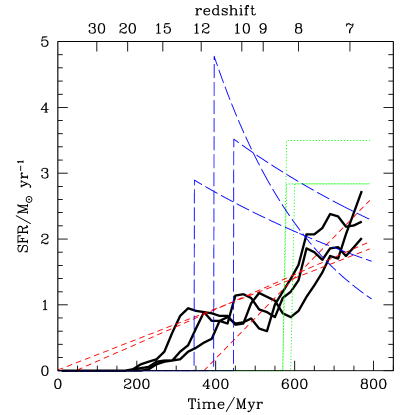
Figure 1: Star formation histories of the 3 best-fitting vzw galaxies for Abell 2218 KESR, along with the 3 best-fitting galaxies from each of our one-parameter model SFHs. The SEDs of all models match the data with $\chi^{2}$ per degree of freedom less than unity. The vzw SFHs have been sampled in 20-Myr bins and smoothed with a 100-Myr tophat for readability. The areas under the curves are slightly different, reflecting uncertainty in the total stellar mass. Note that the best-fitting rising model is very similar to the best-fitting simulated model.

To date, efforts to use SED-fitting to infer the physical properties of high-redshift galaxies have generally employed some combination of constant, exponentially decaying, and single-burst star formation histories in order to span the presumed range of possibilities. In general, it has been found that the stellar mass, SFR, and redshift of a galaxy can be fairly well-constrained via this technique while the age, metallicity, and dust extinction cannot. Much of the gain in precision that results from using simulated galaxies in SED-fitting results from the relatively small range of SFHs that actually occur in the simulations.

For example, the solid black curves in Figure 1 show the SFHs of the 3 galaxies from the vzw simulation that yield the best fits to the $z\sim 6.7$ galaxy Abell 2218 KESR, which we will discuss extensively in §5. The SFHs have been sampled in 20-Myr bins and smoothed with a 100-Myr tophat in order to make the plot more readable. All 3 galaxies begin forming stars at $z>15$ and exhibit a SFR that is generally rising. An examination of simulated SFHs at these redshifts shows that steadily rising SFHs are typical. For this reason we consider a constantly-rising model SFH in this work; as we will see, the constantly-rising model reproduces most closely the constraints obtained from the simulated galaxies (Figure 8). This model has to our knowledge not been investigated before.

In order to facilitate comparison with much of the available SED-fitting work that is available in the literature, we investigate three one-parameter model SFHs for each galaxy in addition to simulated SFHs, as described below:

• Exponentially Decaying SFR We generate models with SFR proportional to $e^{-t/\tau}$. We use four values of $\tau$ logarithmically spaced between 10 and 795 Myr, roughly the age of the universe for our most distant object. Each of these SFHs is sampled at 23 ages $t$ evenly spaced between 10 and 1000 Myr.

• Constant SFR We generate models that have been forming stars at a constant rate $\dot{M_{*}}$ for $t$ Myr. For $t$ we sample 41 ages that lie between 10 and 1000 Myr, and for $\dot{M_{*}}$ we sample 45 SFRs that lie between 0.2 and 30.0 $M_{\odot}\mbox{ yr}^{-1}$.

• Constantly Rising SFR In the constantly rising SFH, a galaxy’s SFR is proportional to its age. While a rising SFH can clearly not be maintained for all galaxies until low redshifts, it arises fairly generically for high-redshift galaxies in hydrodynamic simulations (Finlator et al., 2006). We generate models in which each galaxy’s SFR has been rising at a constant rate for $t$ Myr, where for $t$ we have sampled 41 ages that lie between 10 and 1000 Myr.

For each star formation history, we have generated models with masses in the range $\log(M_{*}/M_{\odot})\in[7.5,10.5]$ and metallicities $Z_{*}/Z_{\odot}\in(0.005,0.07,1.0,2.5)$. These SFHs are then put through the Spoc formalism, in order to determine the probability distribution of physical properties. During the fitting, we require that the oldest star of a given model is not older than the age of the universe at the model’s redshift.

4 Performance of Spoc

4.1 Self-Consistency Test

We begin by testing that Spoc recovers the (known) properties of simulated galaxies. This serves to both test the algorithm and quantify its intrinsic uncertainties. To do so, we take the 73 galaxies that are resolved by our vzw simulation at $z=6.5$, and determine how accurately we can recover their intrinsic physical properties using model galaxies from the $z=6$ and $z=7$ outputs as inputs to Spoc. While the model and sample galaxies are not strictly independent in this test (all but the least massive galaxies at $z=6.5$ correspond to at least one ancestor in the $z=7$ output and descendant in the $z=6$ output), the galaxies are evolving rapidly enough that these populations are effectively independent. The test-case and model galaxies are compared in 6 bands from $i$-band to IRAC 4.5$\mu$m (the same ones applied to Abell 2218 KESR in §5), where we assume a 0.15 magnitude uncertainty in each band. The test-case galaxies are reddened with a fiducial dust extinction $A_{V}=0.6$ via the Calzetti et al. (2000) law. We apply Spoc to these test-cases using each of the different extinction curves mentioned in §3.1 in order to investigate the systematic uncertainties resulting from our ignorance of the appropriate extinction curve for high-redshift galaxies. During the fitting, redshift space is sampled by perturbing each model galaxy over a grid extending to $\Delta z=0.5$ so that we sample the range $z\in[5.5,7.5]$; $A_{V}$ is sampled over the range $A_{V}\in[0,1]$.

Spoc constrains six quantities: $M_{*}$, SFR, $A_{V}$, $Z_{*}$, age, and redshift. The definitions of $M_{*}$ and redshift are self-evident. $A_{V}$ is defined in terms of the Calzetti et al. (2000) reddening presciption. For the purposes of this work, metallicity $Z_{*}$ is defined as the mean mass fraction of metals in the galaxy’s stars; this is useful in determining what metallicity to choose during population synthesis modeling. Although metallicity is not the dominant factor in determining a galaxy’s SED, the fact that the vzw model reproduces the mass-metallicity relation of star-forming galaxies at $z\sim 2$ (Erb et al., 2006; Davé et al., 2006b) as well as for the host galaxy of GRB050904, which is located at $z=6.295$ (Berger et al., 2006; Kawai et al., 2006), leads us to believe that this model’s predictions for the metallicities of observed reionization-epoch galaxies are plausible (Finlator et al. 2007, in prep.). We define a galaxy’s age as the mass-weighted mean age of its star particles; this is more meaningful than the more commonly-used age of the oldest star, which is both difficult to constrain observationally and difficult to predict owing to the stochastic nature of our simulations’ star formation prescription. We define a galaxy’s SFR as the average over the last 100 Myr leading up to the epoch of observation; if none of a galaxy’s stellar mass is older than 100 Myr then the age of the oldest star is used. This metric is found to correlate more tightly with rest-frame UV flux than averages over a shorter time-baseline for the numerically simulated SFHs.

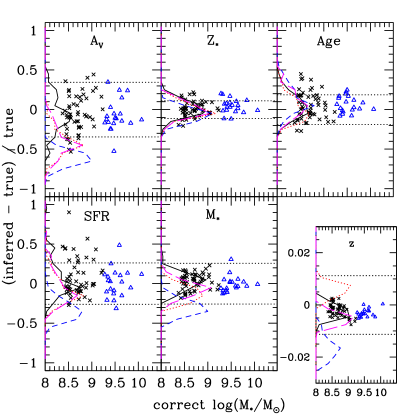
Figure 2: Fractional error in inferred physical properties of $z=6.5$ vzw galaxies as determined using the $z=6.0$ and $z=7.0$ galaxies as models in Spoc. First we considered the case in which both test-case and model galaxies are reddened via the Calzetti et al. (2000) extinction curve. For this run, black crosses and blue triangles denote test galaxies from the $16h^{-1}{\rm Mpc}$ and $32h^{-1}{\rm Mpc}$ volume simulations, respectively; the solid black histogram denotes their combined distribution; and dotted lines indicate mean fractional $1\sigma$ uncertainties computed by Spoc. We then compared the same test-case galaxies (reddened with the same extinctinction curve) to models with the same SFHs but using different dust laws. From these runs, the dotted red, short-dashed blue, and long-dashed magenta histograms correspond to the cases where the models were reddened with the Cardelli et al. (1989), Gordon et al. (2003), and Charlot & Fall (2000) laws. With few exceptions, the best-fit values are within 50% and $2\sigma$ of the correct values. Stellar mass and redshift are recovered remarkably accurately.

First we consider the case in which the test-case and model galaxies are both reddened via the Calzetti et al. (2000) extinction curve. For this case, the points in Figure 2 show how the fractional error in the six inferred properties varies with stellar mass and the solid black histogram gives their combined distribution. The dotted lines indicate the mean formal $1\sigma$ uncertainties; these are computed directly from the probability densities that are returned by Spoc rather than from the scatter in the points. In general, the recovered physical parameters lie within 50% and $2\sigma$ of the correct values, suggesting that our SED-fitting technique is indeed self-consistent. The fact that the formal uncertainties are at least as large as the scatter (and, in some cases, are somewhat larger) suggests that the formal uncertainties are sufficiently conservative.

The most accurately (and precisely) recovered parameter is redshift. The high accuracy in this case owes to the fact that the $I_{814}$, $z_{850}$, and $J_{110}$ fluxes tightly contrain the position of the Lyman break, which itself results from the Madau (1995) prescription for IGM absorption.

Stellar mass is recovered with 20% accuracy, owing primarily to the fact that the rest-frame optical flux is generally dominated by numerous long-lived, low-mass stars whose mass-to-light ratio is relatively insensitive to age and dust extinction. Additionally, as we will show in Figure 3, the lack of a significant systematic offset in the recovered stellar masses owes to the similarity between the SFHs of the test-case and model galaxies.

Metallicity is also accurately recovered. This is expected given that there is a tight mass-metallicity relation in the simulations (the $1\sigma$ scatter is 15%) that does not vary strongly with redshift (Davé et al., 2006a, b), and the fact that the test galaxies and models came from the same simulations. Without this implicit prior, metallicity cannot be tightly constrained from broadband photometry (Papovich et al., 2001; Schaerer & Pelló, 2005).

Turning to SFR, we expect a reasonably accurately inferred SFR given the tight correlation between SFR and stellar mass that the simulated galaxies obey (Finlator et al., 2006; Davé et al., 2006a); in other words, if the redshift is known and the stellar mass can be constrained from the rest-frame optical flux, then the SFR is already constrained to within a factor of two regardless of the rest-frame UV flux. Figure 2 bears this out. In detail, SFR is somewhat less accurately recovered than stellar mass owing to the degeneracies with age and $A_{V}$—in fact, a close inspection reveals that galaxies with underestimated SFR have overestimated $A_{V}$ and vice-versa.

Age is accurately recovered owing largely to the small range of SFHs that occur in our simulations. Just as only a small range of metallicities remains available once the stellar mass is constrained, a relatively small range of ages is available once the redshift and stellar mass are constrained (Figure 1).

If we relax the assumption that we know the correct form of the dust extinction curve, we find systematic effects up to the $\approx 50\%$ level. In Figure 3, the dotted red, short-dashed blue, and long-dashed magenta histograms correspond to the cases where the models were reddened with the Cardelli et al. (1989), SMC bar (Gordon et al., 2003), and Charlot & Fall (2000) laws while the test-cases were reddened with the Calzetti et al. (2000) law as before. Metallicity and age are not strongly affected because these are tightly constrained by the combination of stellar mass and redshift. In contrast, $A_{V}$, $M_{*}$, and SFR are underestimated for the other curves by up to 60% while the photometric redshifts are systematically off by up to 2%, with the the SMC law yielding the largest underestimates. These discrepancies owe to the varying slopes of the extinction curves: Steeper extinction curves require less overall dust (i.e., lower $A_{V}$) and redder rest-frame UV colors (i.e., lower SFR, and thus lower stellar mass in our simulations) in order to match a given observed rest-frame UV color. Similarly, photometric redshifts are systematically off because the extra suppression of rest-frame UV flux that results from an overly steep extinction curve can be partially cancelled out by underestimating the galaxy’s redshift.

In summary, stellar mass, metallicity, age, and SFR can simultaneously be recovered by Spoc when numerically simulated models are used owing to the existence of implicit priors on these parameters. Any remaining discrepancy between the observed and model UV fluxes is minimized by the choice of $A_{V}$, which is also relatively accurately recovered. Thus, our SED-fitting technique is indeed self-consistent. However, if the slope of the assumed dust extinction curve is incorrect then the resulting best estimates of the physical parameters may be off by up to $\approx 50\%$ while the photometric redshift may be off by up to $2\%$. These systematic uncertainties are generic to studies of high-redshift galaxies that employ SED-fitting and are unrelated to uncertainties that result from our ignorance of the correct form of high-redshift SFHs. Since it is the latter aspect that we are currently trying to constrain, we do not further consider SED-fitting errors.

4.2 Comparison With One-Parameter Models

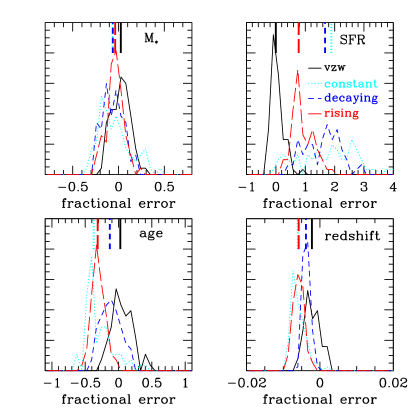
Figure 3: Comparison of the distribution of fractional errors in the inferred physical properties of the galaxies from Figure 2 when assuming different SFHs in Spoc. Redshift error is plotted as $\delta z/(1+z)$. All histograms in a given plot have been normalized to enclose a constant area. Solid black, dotted cyan, short-dashed blue, and long-dashed red curves give the histograms for the simulated, constant, decaying, and rising model sets; the vertical tickmarks at the top indicate the respective medians. Redshift is very well-recovered for all models, stellar mass and age to within 50%, while SFR can be off by large amounts.

It is reassuring but not terribly surprising that Spoc can accurately recover the physical properties of the galaxies that it uses as templates. A more interesting question is how well Spoc can recover galaxy properties using a different SFH than that of the input galaxy, as this illustrates the variations in inferred physical parameters among various assumed SFHs. To address this, we have fit the test-case galaxies that were used in § 4.1 using model sets generated from constant, decaying, and rising SFHs as described in § 3.2.

Figure 3 gives the distributions of fractional errors in the inferred values of stellar mass, SFR, age, and redshift that result when using the different model sets. The vzw case is simply a vertically-binned histogram from Figure 2. Generally, the one-parameter models yield stellar mass and age results that are within 50% of the correct values. The errors for these quantities are generally distributed with slightly larger scatter than the errors from the vzw models and show systematic discrepancies up to the 40% level. The SFRs are overestimated systematically by 50–200% with significantly more scatter than returned by the vzw models; this is clearly the quantity that is most dependent on the assumed SFH. The vzw models systematically underestimate redshift by 0.2% while the one-parameter models are low by 0.5%; the scatters are comparable for all of the models. We briefly discuss results specific to each one-parameter model in turn.

When considering all test-case galaxies together, the constant-SFR models tend to underestimate the age and stellar mass by 40% and 10% respectively while overestimating the SFR by a median factor of 3, the largest discrepancy among the SFHs that we consider. When we split the sample into “massive” and “low-mass” galaxies at $M_{*}/M_{\odot}=10^{9}$, we find that the constant models tend to overestimate the ages of “massive” galaxies by $\sim 20$% while underestimating the ages of low-mass galaxies by $\sim 40$%. In order to match the rest-frame optical measurements, the constant-SFR models then overestimate the SFR for the low-mass and massive galaxies by 100–200% and 0–100%, respectively, with 50% scatter in each case. Stellar masses are underestimated by 20% for the low-mass galaxies and overestimated by roughly the same amount for massive galaxies. This illustrates that uncertainties in parameter recovery are not only dependent on the assumed SFH, but also on the mass.

The decaying models tend to reproduce the stellar mass and age with systematic errors of roughly 10% and scatter comparable to the scatter from the vzw models. These successes are somewhat surprising because the simulated SFHs look nothing like the decaying case. Conversely, the SFRs are higher by a median factor of 2.8, only slightly better than the constant model. The fact that the SFR could be dramatically overestimated while the age, stellar mass, and dust reddening (not shown) are recovered accurately probably owes to our use of 100-Myr average SFRs. When considering all of the stellar mass that has formed in the last 100 Myr, a larger fraction of the O-stars will have evolved off of the main sequence for decaying or constant SFHs than for rising models that show the same 100 Myr average SFR, leading to the result that models with differing SFRs nonetheless produce similar UV luminosities. The broad success of the decaying model despite the input SFHs looking nothing like the decaying case shows that SED fitting can yield interpretations consistent with monolithic collapse models even though the true SFH may be quite different.

The rising models tend to underestimate the age by 10–40% and overestimate the SFR by 40%, though with significant scatter. Both of these offsets are compensated by overestimated $A_{V}$ in such a way that the stellar masses are recovered quite accurately, with $<5$% systematic offset and scatter comparable to what is achieved via the numerically-simulated models. Overall, this model probably recovers the true parameters most faithfully among the one-parameter models, though it is not a dramatic improvement over the others.

In summary, we have shown that Spoc can self-consistently recover the physical properties of the model galaxies that we use in fitting observed high-redshift galaxies. Further, simple one-parameter models are able to recover stellar mass and age to within 50% accuracy and SFR to within a factor of three, although there are systematic offsets at a comparable level. All models yield photometric redshifts with better than 1% accuracy although none of them outperform the numerical models.

4.3 Numerical Resolution

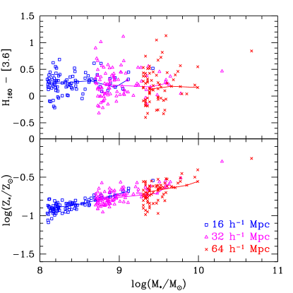
Figure 4: Numerical resolution convergence test I. (Top) Rest-frame UV-optical color versus stellar mass at $z=6$. The blue squares, magenta triangles, and red crosses correspond to the resolved galaxies from the 16, 32, and 64 $h^{-1}{\rm Mpc}$ simulations, respectively; running medians are also given. (Bottom) Stellar metallicity versus stellar mass for the same galaxies. In both cases, the median trend and the scatter do not vary with scale, indicating that the SFHs of our simulated galaxies do not suffer from numerical resolution issues.

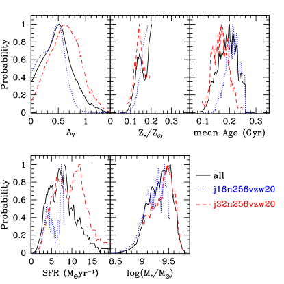
Figure 5: Numerical resolution convergence test II. The dotted blue and dashed red curves give the probability densities for the physical properties of A370 HCM6A as derived from model galaxies from a $16h^{-1}{\rm Mpc}$ and a $32h^{-1}{\rm Mpc}$ simulation volume, respectively, while the solid black curve results from combining the models. All of the probability densities show agreement at the $1\sigma$ level and only the age curves show clear evidence of resolution effects (see text). This figure indicates that our inferred physical properties are not significantly hampered by numerical resolution issues.

The Spoc library of simulated galaxies that we employ is accumulated from simulations at different volumes and resolutions (e.g. in the jvzw case, we use the $16,32,64h^{-1}{\rm Mpc}$ runs). In Davé et al. (2006a), we showed that, down to the adopted stellar mass resolution limit, the physical properties of galaxies are similar at overlapping mass scales between the various simulations. To reiterate this point in a way that is more relevant to the current work, Figure 4 shows how the rest-frame UV-optical color and mean stellar metallicity vary with stellar mass at $z=6$ for resolved ($\geq 64$ star particles) galaxies from our 16, 32, and 64 $h^{-1}{\rm Mpc}$ simulation volumes. In both cases, the trend and the scatter are consistent between the different volumes, giving us further confidence that our simulated SFHs are in fact resolved.

A related way to look for resolution issues is to ask whether Spoc will yield similar answers when it is applied to same-mass galaxies at different resolutions. We now demonstrate that, indeed, Spoc does recover similar parameters for galaxies at different resolutions, and so combining different resolution simulations into a larger set is justified. Of course, one does not need to do so in order to use Spoc, it is merely a convenient avenue to increase the dynamic range spanned by our model galaxies.

For convenience, we study A370 HCM6a as it can readily be fit by our models. We apply Spoc using three sets of models derived from the jvzw simulations: once using models from the $16h^{-1}{\rm Mpc}$ volume (“j16”), once using models from the $32h^{-1}{\rm Mpc}$ volume (“j32”), and once using both sets. A lack of numerical convergence would result in systematic offsets between the probability densities from the first two fits, while the combined result shows how the models from the two volumes combine to yield our full probability density.

Figure 5 shows the derived probability density functions for the various physical parameters that we consider. The ranges agree well, and the best estimates from the j16 and j32 volumes (defined as the means of the probability density functions) are consistent at the $1\sigma$ level. In detail, the j16 models return fits with somewhat lower stellar mass, SFR, and metallicity than the j32 models while the j32 models yield ages that are younger by about 40 Myr. The small offsets in mass, SFR, and metallicity do not indicate resolution problems as they are expected even in the absence of any convergence issues. Briefly, the j16 volume contributes lower mass models owing to the slope of the mass function (at the massive end) and our 64 star particle mass resolution cut (at the low-mass end). On the other hand, the age offset results from a well-known numerical resolution limitation whereby galaxies in lower-resolution simulations take longer to condense beyond a given critical density in order to begin forming stars, yielding younger ages at a given stellar mass and redshift. Fortunately, the offset is comparable to the intrinsic uncertainty on this parameter. We have repeated this test using object SBM03#1 with the 32 and $64h^{-1}{\rm Mpc}$ volumes and found similar results. Hence we do not believe that our results using combined simulation samples are significantly hampered by numerical resolution effects.

5 Test Case: Abell 2218 KESR

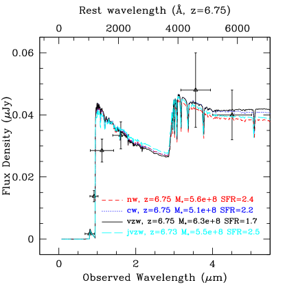
Figure 6: Best-fit spectra from the simulations to the data for Abell 2218 KESR, which we have demagnified by $25\times$ (Kneib et al., 2004). Spectra from the nw, cw, and vzw, and jvzw models are denoted by red dashed, blue dotted, black solid, and long-dashed cyan curves, respectively. All four models produce galaxies whose spectra match Abell 2218 KESR within the errors ($\chi^{2}$ per degree of freedom $<1$).

The triple arc in Abell 2218, dubbed Abell 2218 KESR by Schaerer & Pelló (2005) after its discoverers (Kneib et al., 2004), is probably the best-studied $z>6$ object at present, and its physical parameters have been constrained through SED fitting by various authors. Hence it provides a good test case for exploring the systematics that result from using numerically simulated model galaxies, and comparing to results employing more traditional simple SFHs.

The flux from Abell 2218 KESR can be measured from two lensed images in the Hubble Advanced Camera for Surveys (ACS) $z_{850}$, Wide-Field Planetary Camera 2 (WFPC2) $I_{814}$, and Near-Infrared Camera and Multi-Object Spectrograph (NICMOS) $J_{110}$ and $H_{160}$ bands, and only one image in the Spitzer/IRAC 3.6 and 4.5 $\mu$m bands (the other image is blended with a nearby submillimeter source at IRAC’s spatial resolution). Schaerer & Pelló (2005) note that the fluxes measured by different authors in the optical/near-infrared bands disagree due to the inherent difficulties of measuring photometry from extended arcs, and that the different images of the galaxy do not agree in the Hubble/ACS $z_{850}$ band. Following their suggestion, we use the weighted mean of the two images in the optical/near-infrared bands (their SED1) and impose a minimum 0.15 mag uncertainty in all bands in order to account for differential lensing across the images.

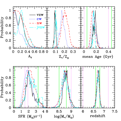
Figure 7: Probability densities for the physical parameters of Abell 2218 KESR based on four numerical simulations assuming different treatments for superwind feedback. Results from the nw, cw, vzw, and jvzw models are given with dashed red, dotted blue, solid black, and long-dashed cyan lines, respectively. Solid green and dotted magenta boundaries denote ranges inferred by Egami et al. (2005) and Schaerer & Pelló (2005), respectively (the lower limit to stellar mass obtained by Schaerer & Pelló (2005) is 7.7). Each curve has been normalized to unit area and then scaled so that the three models fit on the same plot. All of the best-fit physical parameters except metallicity (see text) are robust to changes in the superwind feedback treatment.

5.1 Modeling Uncertainties: Outflows and Dust

Figure 6 shows that the SEDs of the best-fitting model galaxies from our three galactic outflow recipes and two cosmologies all reproduce the observations with reduced $\chi^{2}<1$. Moreover, they are remarkably similar. All four models possess a very blue rest-frame UV continuum owing to young age and low metallicity as well as a pronounced Balmer break owing to the presence of older stars. The best-fit parameters are similar, indicating that the simulation’s ability to reproduce the observations is robust to the choice of superwind feedback prescription and detailed cosmological parameters (to the extent of the variations considered). This result is akin to the findings from studies employing one-parameter model SFHs that good fits can be obtained via a variety of assumed SFHs and metallicities.

To quantify this point, Figure 7 and Table 1 show how the derived probability densities for the physical parameters of Abell 2218 KESR depend on the choice of wind model. The entries in Table 1 list the mean and variance of the histograms shown in Figure 7. Each curve in Figure 7 has been normalized to unit area and then scaled so that all four curves fit on the same plot.

All of the derived physical parameters except $Z_{*}$ are remarkably robust to our choice of superwind feedback prescription. Generally, the data seem consistent with negligible dust reddening, a mean stellar age of 100–200 Myr, SFRs of 1–3 $M_{\odot}\mbox{ yr}^{-1}$, a stellar mass of 3–8$\times 10^{8}M_{\odot}$, and a redshift $z\sim 6.7$, in good agreement with other determinations (Egami et al., 2005; Schaerer & Pelló, 2005). The tightness of the constraints on the various intrinsic physical parameters results from the relatively narrow range of SFHs experienced by the galaxies in the simulations. By contrast, the uncertainty in the inferred redshift is determined by our treatment of IGM extinction since the inferred redshift is dominated by the position of the Lyman-$\alpha$ break.

Comparing the results from the models in detail, both the cw and nw models are less efficient at suppressing star formation via outflows. For this reason, at fixed number density (or equivalently, dark matter halo mass) the cw and nw model galaxies have formed more stars, retained more of their metals, have a higher SFR, and are older (Davé et al., 2006a). Similarly, at a given stellar mass, the vzw galaxies are younger, have expelled a larger fraction of their heavy elements, and for these reasons require more dust reddening in order to match a given observed colour owing to the age–metallicity–dust degeneracy. The jvzw models give results that are the similar to the vzw results owing to the similar feedback treatment. However, the lower values used in the jvzw simulation for the cosmological parameters $\Omega_{m}$ and $\sigma_{8}$ delay the growth of structure at early times, yielding fewer model galaxies for us to match against observations for a given simulated volume. As a result, parameter space is less well-sampled and the probability density curves (notably $A_{V}$) exhibit more stochasticity.

Next to stellar mass and redshift, the mean stellar metallicity is the most tightly constrained parameter, followed by the mean age and SFR. Metallicity is the only parameter for which the different wind models disagree at the $>1\sigma$ level. That the models could agree on all of the derived parameters except for the metallicity reflects the fact that the effect of metallicity on the photometry is small compared to the effect of stellar age (Schaerer & Pelló, 2005). On the other hand, the tightness of the metallicity constraint follows from the tight mass-metallicity relation that the simulation predicts (§ 4). Thus, the apparent disagreement between the metallicity constraints is simply a reflection of the tight priors imposed by the different simulations combined with the robust constraints on stellar mass. Note that because the vzw model agrees the best with the distribution of metals in the IGM (OD06) and the mass-metallicity relationship of star-forming galaxies (Davé et al., 2006b), it probably makes the most believable prediction of Abell 2218 KESR’s mean stellar metallicity.

We investigated the effect that varying the dust prescription has on the derived physical parameters and found, in agreement with Schaerer & Pelló (2005), that this has no significant effect on the derived physical parameters other than $A_{V}$ when the simulated models were used. The derived $A_{V}$ were roughly 0.1 mag lower for the Cardelli et al. (1989) and Charlot & Fall (2000) laws; these differences are expected given the extra extinction imposed at rest-frame UV wavelengths in the former case and (similarly) for younger stars in the latter case. The total amount of light removed by dust extinction, which can be regarded as a prediction of the total infrared luminosity, is roughly $10^{10}L_{\odot}$, independent of the assumed dust prescription.

Two groups have previously published constraints on this object’s properties. Egami et al. (2005) employed a uniform sampling of single-parameter SFHs; their results are given in Table 1 and by the solid green vertical lines in Figure 7, where we have converted their derived SFR and $M_{*}$ to values appropriate for a Chabrier IMF. It is clear that their constraints are entirely consistent with our own, although the tight intrinsic correlations between physical parameters in the simulated models allow us to impose tighter constraints on all of the derived parameters. In the second work, Schaerer & Pelló (2005) exhaustively examined the systematics of assumptions regarding SFH and template spectra with the goal of bracketing the most likely parameter space. Their constraints, given by the dotted magenta vertical lines and listed in 1, are also consistent with ours. Hence our simulations, despite a different generic form for their galaxies’ SFHs than has been assumed in previous investigations, can reproduce the properties of Abell 2218 KESR equivalently well.

5.2 Comparison to One-parameter SFHs

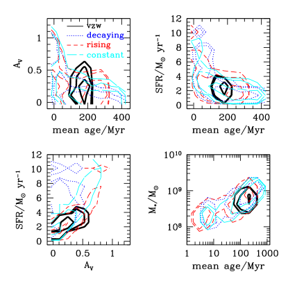
Figure 8: Best-fit combinations of age, extinction, and and SFR for 1000 Monte Carlo re-observations of Abell 2218 KESR. The solid black, dotted blue, short-dashed red, and long-dashed cyan contours enclose 68%, 95%, and 99% of the best-fit solutions for the vzw, decaying, rising, and constant model sets, respectively. The vzw models allow for the tightest constraints to be placed. Interestingly, the $1\sigma$ best-fit intervals from the constantly-rising SFH are very close to the simulation result.

Efforts to constrain the physical properties of high-redshift galaxies via SED-fitting invariably encounter a host of degeneracies between the best-fit parameters, the most difficult of which is certainly the age-extinction-SFR degeneracy (Shapley et al., 2001; Papovich et al., 2001; Shapley et al., 2005). Generally, young stellar population age, high SFR, and low dust extinction all yield bluer photometric colours while old age, low SFR, and high dust extinction all yield redder photometric colours. These degeneracies also contribute to the uncertainty in the inferred stellar mass via the stellar age-stellar mass degeneracy, whereby older populations have a higher mass-to-light ratio, yielding a higher stellar mass at a given measured flux density. Compounding the problem, there are a number of ways in which the best-fit physical properties depend on any assumptions that are made regarding the shape of a galaxy’s star formation history (Shapley et al., 2005). Numerical simulations, in contrast, provide tight relationships between galaxy star formation rate, stellar mass, and metallicity (from which extinction may be inferred). These predicted relationships translate into tighter constraints on physical parameters that depend strongly on the shapes of the trial SFHs.

In order to quantify how effectively the simulations reduce well-known degeneracies in best-fit parameters, we generated 1000 Monte Carlo re-observations of Abell 2218 KESR by adding scatter to the photometric measurements in a way that was consistent with the reported observational uncertainties. For each data set, we then determined the best-fit parameters from the vzw models as well as from the decaying, rising, and constant SFH models. Figure 8 shows the locus of best-fit parameters in several famously degenerate projections of parameter space. The solid black, dotted blue, short-dashed red, and long-dashed cyan contours enclose 68%, 95%, and 99% of the best-fit solutions for the vzw, decaying, rising, and constant model sets, respectively.

The expected degeneracies that result from one-parameter SFHs are easy to see in each panel of Figure 8. At the young end, each of the one-parameter models includes a parameter space corresponding to a galaxy that has formed all of its stars in a rapid burst lasting less than 100 Myr. Our use of 100-Myr average SFRs guarantees these models a high SFR ($\geq 4M_{\odot}\mbox{ yr}^{-1}$). Because these models are very young, they are intrinsically blue and can require high dust reddening ($A_{V}\leq 1$ mag) to match the observations. Additionally, their young ages guarantee that their observed optical flux is dominated by short-lived O and B stars with low mass-to-light ratios, leading to low inferred stellar masses. These dramatic burst-dominated models have no analogue in the simulations.

The old end is dominated by the constant-SFR models, equivalent to the $\tau\rightarrow\infty$ limit of the decaying models. These models are characterized by intrinsically red colours and high mass-to-light ratios, leading to low dust extinctions and high stellar masses. The oldest of these fits requires the galaxy to have been forming stars at $\approx 1M_{\odot}\mbox{ yr}^{-1}$ when the universe was less than 10 Myr old; our simulations cannot produce this because gas densities have not grown high enough to support such SFRs at such early times.

At the $1\sigma$ confidence level, the one-parameter model that most closely approximates the simulated galaxies is the rising SFH model, albeit with a preference for somewhat older ages. Returning to Figure 1, we see that this is expected because the simulated galaxies’ SFHs are generically characterized by a slowly rising SFR at these redshifts. Conversely, at the $\ga 2\sigma$ level, the constantly rising SFH model allows for a wider range of models that have no analogues in the simulations. The relatively small range of simulated galaxy SFHs typified by the examples in Figure 1 leads directly to the relatively tight range of inferred ages for the solid contours in Figure 8. Assuming that Abell 2218 KESR is located at $z=6.75$, the SFHs in Figure 1 suggest that it may have formed its first stars before $z=15$, with (10%, 50%) of its stars in place by $z=$(11,8); in other words, roughly half of the best-fitting models’ stars at the epoch of observation are over 150 Myr old. This relatively old population readily accounts for the pronounced Balmer break that is visible in Figure 6, and is typical in our simulations.

In summary, a key point of this paper is demonstrated by the fact that, in each panel of Figure 8, the confidence intervals obtained from simulated galaxies fall well within the range described by the complete set of one-parameter model SFHs, while yielding the tightest constraints. The tighter constraints owe to the relatively small range of SFHs and the tight correlations between the various parameters that generically occur in hierarchical simulations of galaxy formation. This illustrates that, if the simulations are broadly correct, the physical properties of high-$z$ galaxies can be more precisely constrained using Spoc. However, since at present the simulations are largely untested at these epochs (modulo the broad successes in Davé et al., 2006a), it may be more appropriate to regard the tight simulation constraints as predictions to be tested against future observations.

5.3 The Importance of Rest-Frame Optical Data

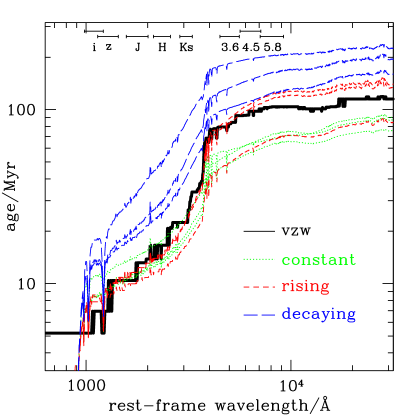
Figure 9: Light-weighted median age of A2218 KESR versus rest-frame wavelength. The single solid curve corresponds to the best-fitting vzw model while the dotted green, short-dashed red, and long-dashed blue curves correspond to the three best-fitting constant, rising, and decaying models, respectively. The ranges at the top of the figure indicate the full width at 20% of maximum response for an object located at $z=6$. The specific one-parameter models whose spectra are considered in Figure 9 are the same as the models in Figure 1 except that we include only the best-fitting vzw model for clarity. Generally, measurements shortward of the Balmer break sample light from stars that are 50-100 Myr old whereas measurements in rest-frame optical wavelengths constrain older populations.

In this work we focus on reionization-epoch objects for which rest-frame optical measurements are available because the rest-frame optical flux is dominated by relatively low-mass stars whose mass-to-light ratio evolves slowly relative to the stars that dominate the rest-frame UV. For reasonable SFHs, this allows tighter constraints to be placed not only on the galaxy’s stellar mass, but also on its SFH. To quantify this point, Figure 9 plots the light-weighted median age of A2218 KESR versus rest-frame wavelength for the SFHs in Figure 1. For example, a point at 2000 Å and 15 Myr indicates that, for that model, 50% of the photons with rest-frame wavelength of 2000 Å are emitted by stars that are 15 Myr old or younger.

For all of the models that we consider, photons from bluewards of the Balmer break are generated by stars that are under 100 Myr old. This is expected since B stars live roughly 100 Myr (Iben, 1967) and justifies the use of rest-frame UV flux as a constraint on the current SFR. Conversely, it explains why rest-frame UV data do not constrain a galaxy’s SFH prior to $\approx 100$ Myr before the epoch of observation. By contrast, data from longer wavelengths sample the SFH at earlier epochs because the stars that dominate these wavelengths live much longer. In the case of A2218 KESR, the constant and decaying models in Figure 9 suggest that rest-frame optical data constrain the galaxy’s SFH roughly 80 and 200 Myr before the epoch of observation, while the rising and vzw models fall in between these limits; the differences probably owe to the detailed interplay between the slope of the SFH and the rate at which low-mass stars fade. It is possible that the rough agreement in the optical portion of Figure 9 explains the tendency of all of the best-fit models in Figure 1 to be in rough agreement with each other during the interval $z\approx 8\rightarrow 6.7$ even though they diverge prior to $z=8$. Note that this agreement is nontrivial given that all of the one-parameter models can in principle match the observations with burst-like solutions (Figure 8). Most importantly, it highlights the potential of rest-frame optical measurements redwards of the Balmer break to constrain the SFH for reionization-epoch galaxies.

6 A Sample of Reionization-Epoch Galaxies

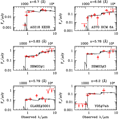
Figure 10: Spectra of the best-fitting model galaxies overplotted on the measured photometry. In cases where spectroscopic redshifts are available this has been forced; in other cases (Abell 2218 KESR and Y05#7ab) we used the photometric redshifts. Horizontal error bars indicate the full width of each filter at 20% of maximum response. The bottom and top horizontal axes give the observed and rest-frame wavelengths. Using the numerically-simulated SFHs with the Bruzual & Charlot (2003) models, we obtain satisfactory fits in all cases and excellent fits in 5 cases.

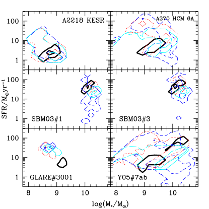
Figure 11: Contours enclosing 68 and 99% of the solutions found for the various galaxies given the various SFHs that we inspected. Thick solid black, dotted red, solid cyan, and dashed blue curves correspond to the jvzw, rising, constant, and decaying SFH models, respectively. In all cases but GLARE#3001, the jvzw models yield results that are generally consistent with the one-parameter model SFHs while allowing for equally-tight or tighter uncertainties.

While the example of Abell 2218 KESR is illustrative, the ultimate purpose of Spoc is to constrain physical parameters for a large sample of galaxies, in order to characterize the observed galaxy population and to constrain the underlying galaxy formation model. To illustrate the sort of insights gained using Spoc, we apply it to a sample of observed $z>5.5$ objects that have published broadband photometry in the rest-frame UV and optical bands. For each object, we used Spoc to determine its best-fit physical parameters with the jvzw, constant, rising, and exponentially-decaying models. For objects whose redshift has been measured spectroscopically, we run Spoc twice: once with the redshift constrained to the measured value and once with the redshift left as a free parameter. The first run allows more accurate derivations of the physical parameters, while the second enables us to study the accuracy of Spoc’s photometric redshifts.

Table 2 compares the means and 95% confidence intervals for the various physical parameters of each galaxy that result from the various models, while Figure 11 shows the 68 and 99% contours in the $M_{*}$-SFR space for the same models. While fitting with one-parameter models, we confirmed that the probability density varies only weakly with $Z_{*}$ (Papovich et al., 2001); for this reason we have omitted $Z_{*}$ from Table 2. Our simulations, combined with Spoc, suggest that all of the objects have $0.1\la Z_{*}/Z_{\odot}\la 0.3$ (Davé et al., 2006a).

Figure 10 compares the synthetic spectra of the best-fit jvzw models with the published rest-frame UV through optical data for our sample. Table 2 shows that we obtain very good fits ($\chi_{\nu}^{2}\la 2$) with the simulated library in all cases except for the unusual object GLARE#3001. Note that these spectra and $\chi_{\nu}^{2}$ values are purely representative; in practice we obtain physical constraints through the Bayesian analysis described in §2 rather than by simply examining the best-fitting model. It is encouraging that the fits obtained from our simulated galaxy library are generally equally as compelling, in terms of goodness-of-fit measure $\chi_{\nu}^{2}$, as the fits that result from the one-parameter SFH model libraries.

Taken together, these findings strongly support the idea that most observed reionization-epoch galaxies possess theoretical analogues within our simulations. However, some of these objects show minor discrepancies that may be hinting at some failing in the models. Given the currently large observational uncertainties it is difficult to place robust constraints on the models, but it is nevertheless worthwhile to discuss each of these systems in detail in order to illustrate how Spoc can be used to both reveal physical characteristics as well as test the underlying model.

A370 HCM 6A: We have taken the photometric data and errors in the observed R,Z,J,H,K’, and Spitzer/IRAC bands from Chary, Stern & Eisenhardt (2005, hereafter CSE05), and we have adopted their lensing magnification factor of 4.5. The measured $4.5\mu$m flux is anomalously large; CSE05 interpret the excess over the inferred stellar continuum as H$\alpha$ emission line flux and derive an SFR of $140\pm 90M_{\odot}\mbox{ yr}^{-1}$. In our simulations galaxies at $z=6.5$ that possess this object’s 3.6$\mu$m flux are forming stars at 2–12$M_{\odot}\mbox{ yr}^{-1}$. Since such systems are not expected to produce H$\alpha$ equivalent widths that would contribute significantly to the broad-band flux, we adopt the uncorrected 4.5$\mu$m measurement. We verified that, if we use the H$\alpha$-corrected 4.5$\mu$m flux obtained by CSE05, the inferred SFR drops from $6.1\pm 2.3$ to $4.9\pm 1.9M_{\odot}\mbox{ yr}^{-1}$; this value is in conflict with the assumed line strength as expected. The $8.0\mu$m limits quoted in the text of CSE05 are different from the limit plotted in their Figure 2; we adopt the less restrictive limit from the Figure.

When we do not enforce the spectroscopic redshift, the photometric redshift $5.9\pm 0.4$ is dominated by the $R-Z^{\prime}$ limit and is roughly $1.5\sigma$ below the spectroscopic redshift; the formal redshift uncertainty is dominated by the size of the $R-Z^{\prime}$ baseline. Although the one-parameter models yield more accurate photometric redshifts in this case, the difference is comparable to the formal uncertainty and we regard it more as a coincidence than as a clue to the SFH of this object. A more accurate photometric redshift would require us to include the unpublished measurement in $I$ and an accurate $Z^{\prime}$ transmission curve; we have used the SDSS $z^{\prime}$ profile because a transmission curve for the $Z^{\prime}$ measurement used by Hu et al. (2002) is not available.

The fits that we obtain are very good, although we confirm that the 4.5$\mu$m measurement is difficult to interpret as purely stellar continuum emission. In fact, even without the anomalous $4.5\mu$m flux the UV continuum is difficult to understand owing to the dip at $K^{\prime}$ (Schaerer & Pelló, 2005), and the measured Ly$\alpha$ flux is difficult to reconcile with the observed Ly$\alpha$ luminosity function at $z\sim 6.5$ (Malhotra & Rhoads, 2004; Kashikawa et al., 2006). Thus, until more precise measurements of this object are available, any inferences regarding its physical properties should probably be regarded as suggestive.

With these caveats in mind, we find that using the simulated models yields inferred stellar mass, SFR, and $A_{V}$ that are fully consistent with previous derivations as well as with the one-parameter model SFHs. The range of stellar masses allowed by the jvzw models nicely brackets the range between the emission line-dominated and stellar continuum-dominated solutions suggested by CSE05, and the range of SFRs is consistent with the derivation of Hu et al. (2002) based on the Ly$\alpha$ line and well below the inferred H$\alpha$-based SFR of CSE05. Turning to the one-parameter models, the widest uncertainties for all of the parameters are provided by the decaying model, with the results from the constant and rising models spanning a somewhat smaller subset of this space. The results from the rising model are generally the closest match to the jvzw models although they permit a somewhat larger range of SFR; these are burst-like models that have no analogue in our simulations.

SBM03#1, SBM03#3, GLARE#3001: We adopted the measured broadband fluxes and spectroscopic redshifts for these objects from Tables 1 and 2 in Eyles et al. (2005). Object SBM03#1 is the same as object #1ab in Yan et al. (2005). Comparing the derived fluxes in these two papers, we find disagreement at the $\approx 1\sigma$ level in the ACS $i_{775}$, $z_{850}$, and NICMOS $H_{160}$ bands. To be conservative, we therefore impose a minimum uncertainty of 0.15 mag in all bands for these objects. When fitting for the photometric redshifts we include the $i_{775}$ fluxes; otherwise we exclude this datum following Eyles et al. (2005). Figure 10 shows that we obtain an excellent fit for SBM03#1 and satisfactory fits for SBM03#3 and GLARE#3001, with the chief difficulty in the latter objects being the anomalous fluxes in $K_{S}$ as noted by Eyles et al. (2005).

For objects SBM03#1 (Dickinson et al., 2004; Stanway et al., 2004a, 2003) and SBM03#3 (Bunker et al., 2003; Stanway et al., 2003) Spoc deduces stellar masses of $\approx 10^{10}M_{\odot}$ and mean ages that include the range 100–300 Myr irrespective of the assumed SFH, consistent with the findings of Eyles et al. (2005). The minimum age for each model is older than the ages for the other objects in our sample because the small measured uncertainties on the 3.6$\mu$m fluxes for SBM03#1 and #3 create the strongest case for a pronounced Balmer break. In our simulations, such objects are roughly 130–200 Myr old and are forming stars at a healthy 30–60 $M_{\odot}\mbox{ yr}^{-1}$ (both $1\sigma$). The resulting intrinsically blue colours cause Spoc to select moderate dust extinctions $A_{V}$ of 0.4–0.9 and 0–0.1 for #1 and #3, respectively, in order to match their UV continuum slopes. While these SFRs are within the full range inferred via the one-parameter models, they are generally more active and younger than inferred via the decaying and constant models. The discrepancy owes primarily to the fact that the constant and decaying models permit higher SFRs at early times ($z\ga 10$) than occur in our simulations. Because the rising model excludes such early episodes, it yields constraints that are more similar to the results from the jvzw models.

The photometric redshifts for SBM03#1 and #3 are 1–3$\sigma$ below the spectroscopic values for both simulation and one-parameter models, suggesting that unknown systematic uncertainties such as uncertainty owing to inaccurate filter profiles should be folded into the formal uncertainties; in future work an enforced minimum redshift uncertainty of $\delta z/(1+z)\geq 0.02$ seems reasonable.

Object GLARE#3001 is a particularly interesting case because it represents the worst fit for all our models. This object shows a relatively flat SED with little evidence for a Balmer break (Figure 10). The photometric redshifts are systematically high although they are accurate at the $1\sigma$ level. Spoc finds that it is perhaps an order of magnitude less massive than SBM03#1 and #3. In our simulations, the analogues to GLARE#3001 are of roughly the same age as the SBM objects while their SFRs are roughly one tenth as large, leading to similarly strong Balmer breaks and dust extinctions. Comparing with the one-parameter model SFHs, Table 2 shows that, for this object, constant and rising models yield masses, SFRs, and ages that are marginally consistent with the results from our simulations (although they are skewed to higher SFR) while decaying models yield extremely young, burst-like fits whose parameters are entirely inconsistent with the jvzw results (this is especially clear in Figure 11).

The chief difficulty in fitting GLARE#3001 is the anomalously high flux measured in $K_{S}$, as noted by Eyles et al. (2005). If real, this would suggest that this is a low-mass objects undergoing a burst. Table 2 shows that the $\chi_{\nu}^{2}$ per degree of freedom is lower for the one-parameter models than for the simulated models, because the one-parameter models have the freedom to produce a higher $K_{S}$ flux through a higher SFR and $A_{V}$ together with a lower stellar mass; galaxies with these combinations of high SFR ($>10M_{\odot}\mbox{ yr}^{-1}$) and low stellar mass ($<10^{9}M_{\odot}$) simply do not occur in our simulations. It would be preliminary to stake the final interpretation of this galaxy on one broadband measurement (particularly one in $K_{S}$), especially since even the one-parameter model fits are not particularly good ($\chi_{\nu}^{2}\ga 3$). But this object does illustrate how Spoc can pick out galaxies that may provide the most stringent tests of galaxy formation models.

Y05#5abc,#7ab: We adopted the Hubble/ACS+NICMOS and Spitzer/IRAC fluxes for objects #5abc and #7ab from the $z\approx 6$ sample in Yan et al. (2005) and imposed a minimum uncertainty of 0.15 mag in all bands as before. Spoc failed to find an acceptable fit for object #5abc, for either simulated or one-parameter model SFHs. This object is evidently a blend of at least three components located at different redshifts and should therefore be fit with multiple components (Yan et al., 2005); however, this is beyond the scope of the present work. We therefore do not show the results from #5abc.

By contrast, we obtain excellent fits for object #7ab. This is somewhat surprising given that #7ab is clearly a mixture of two components (Figure 1 in Yan et al. (2005)), and probably owes largely to the fact that it does not show anomalous single-band fluxes in the way that HCM 6A, SBM03#3, and GLARE#3001 do. The photometric redshift is constrained to $6.2\pm 0.2$, $1.5\sigma$ higher than the photometric redshift determined by Yan et al. (2005) (although they do not quote an uncertainty). Stellar mass is relatively poorly constrained owing to the relatively low signal-to-noise in the observed 3.6$\mu$m band. As Figure 11 shows, when we apply Spoc with our simulated models, the poorly-constrained stellar mass leads directly to a poorly-constrained SFR. Comparing with the one-parameter models, we find that these span an even larger (overlapping) space. This object illustrates the importance of high-quality near-infrared data in order to understand the physical properties of high-redshift galaxies.

Yan et al. (2005) applied exponentially-decaying models to this object and found a burst-like best-fit solution with a stellar mass of $\log(M_{*}/M_{\odot})=9.5$ (when converted to a Chabrier IMF), little current star formation ($\sim 0.001M_{\odot}\mbox{ yr}^{-1}$), no dust extinction, and an age of 50–100 Myr. The stellar mass is fully consistent with our jvzw results. However, we find disagreement in the inferred dust extinction, SFR, and age because in the simulations galaxies of this stellar mass and redshift are invariably older and are still forming stars. In particular, we expect $A_{V}=0.34\pm 0.24$, $\dot{M_{*}}=9\pm 5M_{\odot}\mbox{ yr}^{-1}$, and age = $175\pm 30$ Myr (1 $\sigma$ uncertainty). Once again, the absence of burst-like models in our simulations constitutes an effective prior that excludes such solutions. When we apply our own exponentially-decaying models to this object we find that the probability density possesses a sharp peak at low ages ($<100$ Myr) and a broad but slightly lower plateau at older ages. So while we formally obtain the lowest $\chi^{2}$ for burst-like models, folding in our simulation prior leads to an older age being preferred. This object is therefore a classic case where simply taking the lowest $\chi^{2}$ among all SFHs results in a substantially different interpretation than that obtained using physically-motivated priors. It will be interesting to see with improved obervations whether or not the simulation prediction ends up being correct.

The sixth column of Table 2 combines $M_{*}$ and $\dot{M_{*}}$ with the age of the universe $t_{H}$ at each galaxy’s redshift into an estimate of the ratio of the present- to past-averaged SFR, $\dot{M_{*}}/(M_{*}/t_{H})=t_{H}/t_{SFR}$. A value of $t_{H}/t_{SFR}$ less than unity indicates a declining SFH whereas a value greater than unity indicates a rising SFH. Eyles et al. (2005, 2006) have previously used this quantity to argue that galaxies that exhibit Balmer breaks at $z\sim 6$ must be experiencing a declining SFH. In contrast, Table 2 indicates that, while this possibility is permitted by the decaying models at the $2\sigma$ level for all but one of the galaxies that we consider, it is by no means required. For our physically-motivated models it is not permitted owing to the generally rising SFHs in our simulations, but in fact even for the decaying models it is not the favored solution when the full range of possibilities is taken into account. Hence we do not find that the presence of a Balmer break requires a declining SFH. The disagreement between our results and those of Eyles et al. (2005) owes partly to the slightly different model sets used in the two analyses, and partly to our employing the full probability densities rather than restricting our attention to the model with the lowest $\chi^{2}$. Most importantly, however, this disagreement emphasizes the fact that the form of the correct SFH is not constrained by the current measurements and hence the conclusions are highly model-dependent.

In these fits, we have not considered the possibility of any AGN contribution to the SEDs. From rest-UV photometry alone it is difficult to rule out this possibility. Fitting power laws of the form $f_{\nu}\propto\nu^{\alpha}$ to their rest-frame UV continua, we obtain slopes in the range $\alpha\in[-0.3,-1.1]$ with a weighted mean of -0.61. These are not significantly different from the slopes inferred by Fan et al. (2001) from 39 quasars at $3.66\leq z\leq 4.77$, with a mean and standard deviation of -0.79 and 0.34, respectively. However, with Spitzer/IRAC photometry the Balmer breaks in A2218 KESR, SBM03#1, SBM03#3, and Y05#7ab are clearly evident. Furthermore, Stanway et al. (2004a) and Bunker et al. (2003) argue that AGN can be ruled out for three of the objects (SBM03#1, SBM03#3, and GLARE#3001) based on upper limits to the flux of the N v doublet at 1240Å, the lack of any X-ray detection, and the relatively small velocity width of the observed Ly$\alpha$ lines ($v_{\mbox{\tiny{FWHM}}}<500\;{\rm km}\,{\rm s}^{-1}$). These arguments also apply to A370 HCM 6A. Additionally, CSE05 note that the latter object is similar to high-redshift Ly$\alpha$ emitters, for which the AGN fraction is constrained to be less than 5% (e.g., Gawiser et al., 2006; Ouchi et al., 2005; Dawson et al., 2004; Wang et al., 2004; Santos et al., 2004). This suggests that AGN do not dominate their rest-frame optical spectra, and emphasizes the usefulness of Spitzer/IRAC measurements for constraining the properties of reionization-epoch objects. Hence it seems reasonable to model all of these objects with stellar population synthesis models alone, as we have done.

In summary, we are usually but not always able to find galaxies within our simulations whose photometry suggests that they could be the theoretical counterpart to observed reionization-epoch galaxies. Using these models as inputs to our SED-fitting engine, Spoc, we obtain physical constraints on the properties of the galaxies that are, in five out of six cases, consistent with the results from one-parameter model SFHs. In the remaining case, the observed SED leads the one-parameter models to prefer burst-like scenarios that do not occur in our simulations. In all cases the tightness of constraints from the simulated models is equal to or better than that from one-parameter model SFHs. Albeit small, this sample of systems illustrates how using Spoc to compare among SFHs can provide insights into the physics of early galaxy formation, and identify unusual galaxies that provide the tightest constraints on such models.

7 Conclusions

In this paper we present a Bayesian SED-fitting engine called Spoc, which provides constraints on the physical properties of galaxies from photometric data. Spoc takes as input a galaxy’s photometry and a set of model galaxy spectra, obtained either by assuming an analytic form for the galaxy’s star formation history or from numerical simulations of galaxy formation, and outputs probability distributions for the physical properties of individual galaxies based on those model priors. Here we compare and explore implications for different models, with an eye towards better constraining the physical properties of high-redshift galaxies.

Because Spoc is intended to test whether predicted SFHs match those inferred from data, it provides constraints on models of galaxy formation that complement comparisons to bulk properties such as galaxy luminosity functions or clustering. A successful model must not only reproduce observed bulk statistics, but must also reproduce the colors of individual galaxies across all observed bands. Galaxies with photometry that cannot be well fit in a given model provide insights into model failings, and ultimately into the physics that drives galaxy formation. Using Spoc it is possible to quantitatively determine how well a particular model matches an individual galaxy. Such a methodology is particularly useful at epochs when only a small number of galaxies are detectable, such as for the earliest galaxies known.

We show that Spoc accurately recovers the input physical parameters of model galaxies when fitted with SFH derived from the simulations themselves, with typical systematic errors less than the formal $1\sigma$ fitting errors. When a simulated galaxy is fit with one-parameter star formation histories or the incorrect extinction model, then larger deviations can occur. Since the true SFH and extinction law are unknown, these deviations can be regarded as systematic errors on the determination of physical parameters. In most cases, such systematic errors are less than 50% in stellar mass, star formation rate, and $A_{V}$, and $\la 2\%$ in redshift.

We then apply Spoc to six galaxies at $z\ga 5.5$ that have published photometry spanning the 4000Å break (which is necessary in order to obtain meaningful constraints on physical properties). We begin with a more in-depth study of Abell 2218 KESR ($z\approx 6.7$), since at present it is probably the best-studied reionization-epoch system, and then apply Spoc to five more galaxies in order to investigate a wider variety of galaxy properties. Our main conclusions are summarized as follows:

• The physical parameters derived for Abell 2218 KESR using our library of simulated galaxies are in line with previous determinations, and those employing various one-parameter SFHs. The formal uncertainties are smaller when using simulated galaxies, because the simulations intrinsically produce a relatively narrow range of SFHs for galaxies at these epochs. The existence of an object with the properties of Abell 2218 KESR at these epochs does not pose a significant challenge to current models of galaxy formation.

• All inferred physical parameters for Abell 2218 KESR except metallicity are remarkably insensitive to the explored choices for superwind feedback model, dust extinction law, and cosmology. The fundamental reason for this is that regardless of such choices, simulations produce a similar form for the SFH of early galaxies. Disappointingly, this means that photometry alone cannot constrain such modeling uncertainties. On the other hand, this means that simulation predictions of physical parameters using Spoc are quite robust. Discrimination between, say, superwind feedback models can be obtained through comparisons with bulk properties such as luminosity functions (as shown in Davé et al., 2006a).

• Exploring a set of six $z\ga 5.5$ galaxies, we find that for five of the systems the simulated galaxies and one-parameter models produce overlapping probability contours and best-fit physical parameters that are formally consistent, and the minimum reduced $\chi^{2}$ is similar between all models. This shows that simulations are usually but not always able to produce galaxies with properties similar to observed $z\sim 6$ systems.

• The spectra of simulated galaxies always show a significant Balmer break, despite the fact that their SFHs are best characterized as constantly-rising (not decaying). The median stellar age is $\approx 120-250$ Myr ($2\sigma$) for all six objects, spanning a range in stellar masses from $\sim 5\times 10^{8}M_{\odot}\la M_{*}\la 2\times 10^{10}M_{\odot}$. Hence the existence of somewhat older stellar populations in these early systems is consistent with simulation predictions.

• The object GLARE#3001 is an outlier that is poorly fit by our simulations, though in fairness the fits with one-parameter models are not optimal either. The best fits tend to favor models with younger stellar ages, lower masses, and higher SFRs than any simulated galaxies, perhaps indicating that this is a galaxy undergoing a burst. However, as discussed in the text, these fits are mainly driven by a high $K_{s}$-band flux. If that data point were confirmed it would suggest that the simulations may be missing some physical process(es) that governs a small fraction of galaxies at this epoch.

Our hydrodynamic simulations of galaxy formation make some clear predictions for the star formation histories of galaxies at these early epochs. In particular, they predict that the stellar mass, star formation rate, and metallicity are all tightly correlated (Finlator et al., 2006; Davé et al., 2006a). Indeed such trends are generically seen in most hydrodynamic simulations of galaxy formation, though not necessarily in semi-analytic models. Our preliminary comparisons to $z\sim 6$ galaxies show that, while the simulations are not necessarily statistically favored over other classes of SFHs, the available data at least do not rule out these simulation predictions. Together with the fact that such simulations can reproduce key bulk properties of early galaxies (Finlator et al., 2006; Davé et al., 2006a), this suggests that models of early galaxy formation are able to reproduce a range of observed properties of galaxies at these epochs.

In this work we have performed the simplest possible spectral synthesis calculations, primarily because our focus has been a comparison between different SFH models. In the future we plan to investigate different population synthesis models (e.g., Maraston et al., 2006), IMFs (e.g. Fardal et al., 2006), and nonstellar contributions to the observed fluxes such as emission lines from HII regions. Eventually we will apply Spoc to a larger sample of galaxies, which will enable a number of interesting investigations. First, the bulk statistics (e.g. stellar mass or star formation rate functions) derived using Spoc can be compared against that directly produced in simulations. While this is partly a circular comparison because simulated galaxies are being used to infer the physical properties, in practice there is no guarantee that consistency will be achieved because the simulated SFHs are quite generic; hence this should provide a stringent test of models of galaxy formation. Second, Spoc can be used to identify populations of galaxies that deviate dramatically from simulation predictions (such as GLARE#3001), in order to isolate which physical processes may be missing in models. In principle this could quantify the contributions from nonstellar emission-dominated sources such as AGN and extremely dusty objects. Finally, the redshift evolution of the galaxy population provides a strong test of models, particularly investigating the dramatic change in the nature of massive galaxies that appears to occur at $z\sim 1-2$ (Papovich et al., 2005).

Spoc is a general-purpose code, in principle able to utilize any type of model that produces detailed galaxy SFHs, be it a hydrodynamic, semi-analytic, or analytic model. In principle there is nothing that restricts Spoc to high redshift use, but in practice other physical phenomena such as AGN contamination may become more important at lower redshifts. Spoc could also provide a useful tool to identify galaxy classes that are not readily reproduced in current models. We are currently planning to make Spoc and our latest library of simulated galaxies publicly available upon publication of this paper. We hope that Spoc will be a useful and flexible tool for conducting detailed comparisons between simulations and observations, as are critical for advancing our understanding of galaxy formation.

References

- Ajiki et al. (2006) Ajiki, M., Mobasher, B., Taniguchi, Y., Shioya, Y., Nagao, T., Murayama, T., & Sasaki, S. S. 2006, ApJ, 638, 596
- Balogh et al. (2001) Balogh, M. L., Pearce, F. R., Bower, R. G., & Kay, S. T. 2001, MNRAS, 326, 1228
- Benítez (2000) Benítez, N. 2000, ApJ, 536, 571
- Berger et al. (2006) Berger, E. et al., ApJ, submitted, astro-ph/0603689
- Bouwens et al. (2004a) Bouwens, R. J., Thompson, R. I., Illingworth, G. D., Franx, M., van Dokkum, P. G., Fan, X., Dickinson, M. E., Eisenstein, D. J., Rieke, M. J. 2004, ApJ, 616, L79
- Bouwens et al. (2004b) Bouwens, R. J., et al. 2004, ApJL, 606, L25
- Bouwens et al. (2006) Bouwens, R. J., Illingworth, G. D., Blakeslee, J. P., & Franx, M. 2006, ApJ, in press, astro-ph/0509641
- Bruzual & Charlot (2003) Bruzual, G. & Charlot, S. 2003, MNRAS, 344, 1000
- Bunker et al. (2003) Bunker, A. J., Stanway, E. R., Ellis, R. S., McMahon, R. G., & McCarthy, P. J. 2003, MNRAS, 342, L47
- Calzetti et al. (2000) Calzetti, D., Armus, L., Bohlin, R. C., Kinney, A. Koornneef, J., & Storchi-Bergmann, T. 2000, ApJ, 533, 682
- Cardelli et al. (1989) Cardelli, J. A., Clayton, G. C., & Mathis, J. S. 1989, ApJ, 345, 245
- Charlot & Fall (2000) Charlot, S., & Fall, S. M. 2000, ApJ, 539, 718
- Chary, Stern & Eisenhardt (2005) Chary, R.-R., Stern, D., & Eisenhardt, P. 2005, ApJL, 635, L5 (CSE05)
- Cuby et al. (2003) Cuby, J.-G., Le Fèvre, O., McCracken, H., Cuillandre, J.-C., Magnier, E., & Meneux, B. 2003, A&A, 405, L19
- Davé et al. (2006a) Davé, R., Finlator, K., & Oppenheimer, B. 2006, MNRAS, accepted, astro-ph/0511532
- Davé et al. (2006b) Davé, R., Finlator, K., & Oppenheimer, B. 2006, to appear in proc. ”Chemodynamics 2006: From First Stars to Local Galaxies”, astro-ph/0608537
- Dawson et al. (2004) Dawson, S., et al. 2004, ApJ, 617, 707
- Dickinson et al. (2004) Dickinson, M., et al. 2004, ApJL, 600, L99
- Drory et al. (2005) Drory, N., Salvato, M., Gabasch, A., Bender, R., Hopp, U., Feulner, G., & Pannella, M. 2005, ApJL, 619, L131
- Dunlop et al. (2006) Dunlop, J. S., Cirasuolo, M., & McLure, R. J., MNRAS, submitted, astro-ph/0606192
- Erb et al. (2006) Erb, D. et al. 2006, ApJ, accepted, astro-ph/0604041
- Egami et al. (2005) Egami, E. et al. 2005, ApJ, 618, L5
- Eyles et al. (2005) Eyles, L. P., Bunker, A. J., Stanway, E. R., Lacy, M., Ellis, R. S., & Doherty, M. 2005, MNRAS, 364, 443
- Eyles et al. (2006) Eyles, L. P. et al. 2006, MNRAS, submitted, astro-ph/0607306
- Fan et al. (2001) Fan, X., et al. 2001, AJ, 121, 31
- Fardal et al. (2006) Fardal, M., Katz, N., Weinberg, D., & Davé, R. 2006, MNRAS, submitted, astro-ph/0604534
- Finlator et al. (2006) Finlator, K., Davé, R., Papovich, C., & Hernquist, L. 2006, ApJ, 639, 672
- Gawiser et al. (2006) Gawiser, E., et al. 2006, ApJL, 642, L13
- González-Serrano et al. (2005) González-Serrano, J. I., Cepa, J., Pérez-García, A. M., Gallego, J., Alfaro, E. J., Sánchez-Portal, M., & González, J. J. 2005, Revista Mexicana de Astronomia y Astrofisica Conference Series, 24, 247
- Gordon et al. (2003) Gordon, K. D., Clayton, G. C., Misselt, K. A., Landolt, A. U., & Wolff, M. J. 2003, ApJ, 594, 279
- Gwyn & Hartwick (2005) Gwyn, S. D. J., & Hartwick, F. D. A. 2005, AJ, 130, 1337
- Haardt & Madau (2001) Haardt, F. & Madau, P. 2001, in proc. XXXVIth Rencontres de Moriond, eds. D.M. Neumann & J.T.T. Van.
- Hu et al. (2002) Hu, E. M., Cowie, L. L., McMahon, R. G., Capak, P., Iwamuro, F., Kneib, J.-P., Maihara, T., & Motohara, K. 2002, ApJL, 576, L99
- Hu et al. (2004) Hu, E. M., Cowie, L. L., Capak, P., McMahon, R. G., Hayashino, T., & Komiyama, Y. 2004, AJ, 127, 563
- Iben (1967) Iben, I. J. 1967, ARA&A, 5, 571
- Idzi et al. (2004) Idzi, R., Somerville, R., Papovich, C., Ferguson, H. C., Giavalisco, M., Kretchmer, C., & Lotz, J. 2004, ApJL, 600, L115
- Kashikawa et al. (2006) Kashikawa N., et al. 2006, astro-ph/0604149
- Kauffmann et al. (2003) Kauffmann, G., et al. 2003, MNRAS, 341, 33
- Kawai et al. (2006) Kawai, N., et al. 2006, Nature, 440, 184
- Kennicutt (1998) Kennicutt, R. C. 1998, ApJ, 498, 541
- Keres et al. (2005) Keres, D., Katz, N., Weinberg, D. H., & Davé, R. 2005, MNRAS, in press
- Kneib et al. (2004) Kneib, J.-P., Ellis, R. S., Santos, M. R., & Richard, J. 2004, ApJL, 568, L75
- Kodaira et al. (2003) Kodaira, K., et al. 2003, PASJ, 55, L17
- Kolatt et al. (1999) Kolatt, T. S. et al. 1999, ApJL, 523, L109
- Kurk et al. (2004) Kurk, J. D., Cimatti, A., di Serego Alighieri, S., Vernet, J., Daddi, E., Ferrara, A., & Ciardi, B. 2004, A&A, 422, L13
- Labbé et al. (2004) Labbé, I., et al. 2006, astro-ph/0608444
- Madau (1995) Madau, P. ApJ, 441, 18
- Malhotra & Rhoads (2004) Malhotra, S. & Rhoads, J. 2004, ApJ, 617, L5
- Malhotra et al. (2005) Malhotra, S., et al. 2005, ApJ, 626, 666
- Maraston et al. (2006) Maraston, C., et al. 2006, ApJ, submitted, astro-ph/0604530
- Martin (2005) Martin, C. L. 2005, ApJ, 621, 227
- McKee & Ostriker (1977) McKee, C. F. & Ostriker, J. P. 1977, ApJ, 218, 148
- Murray, Quatert, & Thompson (2005) Murray, N., Quatert, E., & Thompson, T. A. 2005, ApJ, 618, 569
- Mobasher et al. (2005) Mobasher, B. et al. 2005, ApJ, in press
- Nagao et al. (2004) Nagao, T., et al. 2004, ApJL, 613, L9
- Nagao et al. (2005) Nagao, T., et al. 2005, ApJ, 634, 142
- Night et al. (2005) Night, C., Nagamine, K., Springel, V., & Hernquist, L. 2005, MNRAS, accepted, astro-ph/0503631
- Oppenheimer & Davé (2006) Oppenheimer, B. D. & Davé, R. 2006, MNRAS, in press, astro-ph/0605651 (OD06)
- Ouchi et al. (2005) Ouchi, M., et al. 2005, ApJL, 620, L1
- Papovich et al. (2001) Papovich, C., Dickinson, M., & Ferguson, H. C. 2001, ApJ, 559, 620
- Papovich et al. (2005) Papovich, M. et al. 2005, ApJ, submitted
- Rhoads & Malhotra (2001) Rhoads, J. E., & Malhotra, S. 2001, ApJL, 563, L5
- Rhoads et al. (2003) Rhoads, J. E., et al. 2003, AJ, 125, 1006
- Rhoads et al. (2004) Rhoads, J. E., et al. 2004, ApJ, 611, 59
- Rupke et al. (2005) Rupke, D. S., Veillaux, S., & Sanders, D. B. 2005, ApJS, accepted, astro-ph/0506611
- Santos et al. (2004) Santos, M. R., Ellis, R. S., Kneib, J.-P., Richard, J., Kuijken, K. 2004, ApJ, 606, 683
- Schaerer & Pelló (2005) Schaerer, D., & Pelló, R. 2005, MNRAS, 362, 1054
- Shapley et al. (2001) Shapley, A. E., Steidel, C. C., Adelberger, K. L., Dickinson, M., Giavalisco, M., & Pettini, M. 2001, ApJ, 562, 95
- Shapley et al. (2005) Shapley, A. E., Steidel, C. C., Erb, D. K., Reddy, N. A., Adelberger, K. L., Pettini, M., Barmby, P., & Huang, J. 2005, ApJ, 626, 698
- Shimasaku et al. (2006) Shimasaku, K., et al. astro-ph/0602614
- Smail et al. (2004) Smail, I., Chapman, S. C., Blain, A. W., & Ivison, R. J. 2004, ApJ, 616, 71
- Somerville et al. (2001) Somerville, R. S., Primack, J. R., & Faber, S. M. 2001, MRAS, 320, 504
- Spergel et al. (2003) D. N. Spergel et al., ApJS, 148, 175
- Spergel et al. (2006) D. N. Spergel et al., astro-ph/0603449
- Springel & Hernquist (2002) Springel, V. & Hernquist, L. 2002, MNRAS, 333, 649
- Springel & Hernquist (2003a) Springel, V. & Hernquist, L. 2003a, MNRAS, 339, 289
- Springel & Hernquist (2003b) Springel, V. & Hernquist, L. 2003b, MNRAS, 339, 312
- Springel, Frenk, & White (2006) Springel, V., Frenk, C. S., & White, S. D. M. 2006, Nature, 440, 1137
- Stanway et al. (2003) Stanway, E. R., Bunker, A. J., & McMahon, R. G. 2003, MNRAS, 342, 439
- Stanway et al. (2004a) Stanway, E. R., et al. 2004, ApJL, 604, L13
- Stanway et al. (2004b) Stanway, E. R., Bunker, A. J., McMahon, R. G., Ellis, R. S., Treu, T., & McCarthy, P. J. 2004, ApJ, 607, 704
- Stern et al. (2005) Stern, D., Yost, S. A., Eckart, M. E., Harrison, F. A., Helfand, D. J., Djorgovski, S. G., Malhotra, S., & Rhoads, J. E. 2005, ApJ, 619, 12
- Stiavelli et al. (2005) Stiavelli, M., et al. 2005, ApJL, 622, L1
- Wang et al. (2004) Wang, J. X., et al. 2004, ApJL, 608, L21
- Wang et al. (2005) Wang, J. X., Malhotra, S., & Rhoads, J. E. 2005, ApJL, 622, L77
- Westra et al. (2005) Westra, E., et al. 2005, A&A, 430, L21
- Yan et al. (2005) Yan, H., et al. 2005, ApJ, 634, 109