Snapping Supernovae at $z>1.7$

Abstract

We examine the utility of very high redshift Type Ia supernovae for cosmology and systematic uncertainty control. Next generation space surveys such as the Supernova/Acceleration Probe (SNAP) will obtain thousands of supernovae at $z>1.7$, beyond the design redshift for which the supernovae will be exquisitely characterized. We find that any $z\gtrsim 2$ standard candles’ use for cosmological parameter estimation is quite modest and subject to pitfalls; we examine gravitational lensing, redshift calibration, and contamination effects in some detail. The very high redshift supernovae — both thermonuclear and core collapse — will provide copious interesting information on star formation, environment, and evolution. However, the new observational systematics that must be faced, as well as the limited expansion of SN-parameter space afforded, does not point to high value for $1.7<z<3$ SNe Ia in controlling evolutionary systematics relative to what SNAP can already achieve at $z<1.7$. Synergy with observations from JWST and thirty meter class telescopes afford rich opportunities for advances throughout astrophysics.

1 Introduction

Supernovae play important roles in astrophysics and cosmology, from stellar nucleosynthesis and subsequent star formation, to injection of substantial energy as galaxies form and evolve, to production of neutron stars, black holes, and gamma ray bursts, neutrinos, and subsequent gravitational waves, to use as standardized measures of the expansion history of the universe and probes of dark energy.

Their visible luminosities are so great they can be seen to high redshifts, and certain classes (in particular Type Ia) can be calibrated more accurately than any other astronomical object to provide robust distance measures. For these reasons, supernovae observations are pushing to higher and higher redshifts, looking back over the majority of the history of the universe. Since they become difficult to observe from the ground as their flux redshifts out of the optical window and the terrestrial sky background grows very bright, space based measurements are necessary. Wide field instruments are needed to achieve sufficient numbers to study, and stringent, systematics controlled experiments to derive accurate results. For example, the Supernova/Acceleration Probe (SNAP: Aldering et al. (2004)) is carefully designed specifically to achieve high quality (in both statistics and systematics), well characterized, photometric and spectroscopic observations of thousands of supernovae.

Space extends the reach of a non-cryogenic telescope to 1.7$\mu$m, beyond which thermal noise swamps the astronomical signal. To this wavelength limit the SiII 6300Å spectral feature used for classification of Type Ia supernovae (SNe Ia) can be observed to redshift $z=1.7$. This redshift limit matches extremely well the optimum depth for dark energy investigations, beyond which the sensitivity to the dark energy characteristics fades away (Linder & Huterer, 2003). However, a 2-m class space telescope such as SNAP will observe large numbers of supernovae, both SNe Ia and other types, at redshifts $z>1.7$. For example, the visible flux could be followed out to $z\approx 4$ and the near UV down to 2500Å (SNe Ia have almost no emission $<2500$Å) out to $z\approx 6$.

In this article we investigate the usefulness of space based, wide field observations of SNe beyond $z=1.7$ for cosmology and astrophysics. Section 2 addresses the cosmological impact of extending precision distance measurements to $z>1.7$, including gravitational lensing effects; this will be generally applicable to any standardized candle, not just supernovae. The rates and yield of supernovae of all types are discussed in §3, together with measurement issues such as light curve fitting, redshift determination, Malmquist bias, and supernova typing. Section 4 investigates what we can learn about progenitor age, metallicity, and dust properties, and how this impacts treatment of systematic uncertainties of the $z<1.7$ sample. We summarize in §5 the prospects for using very high redshift SNe (obtained for “free”, and in conjunction with JWST or a TMT) to advance a variety of astrophysical fields.

2 Cosmology beyond $z=1.7$

The discovery of the recent acceleration of the cosmic expansion is a breakthrough in the quest to understand the universe. To reveal the nature of the dark energy responsible for the acceleration requires accurate measurements throughout the accelerating epoch and back into the time of deceleration. However, indefinite extension through the matter dominated, deceleration epoch is of limited use (see, e.g., Linder & Huterer (2003)), with diminished science returns for $z\gtrsim 1.7$. This lack of leverage, together with increased uncertainty – and biasing – from photometric, redshift, and environment measurement errors and gravitational lensing (de)amplification of the source flux, is one of the flaws in seeking to push putative standardizable candles such as gamma ray bursts or gravitational waves to higher redshifts.

2.1 Dark energy

We begin by addressing this question in more detail: could there be some dark energy scenarios where percent level measurements of $z\gtrsim 1.7$ distances are crucial in uncovering the nature of dark energy? On a coarse level the answer is immediately no; we know that structure formed in the universe, in a manner not too different from a universe dominated by matter at $z>2$, so dark energy cannot be dynamically important at high redshift (see Linder (2006b) for details about growth of structure constraints). However it is worthwhile to address this question quantitatively, from the distance perspective, to show that even percent level distance measurements are insufficient.

Let us consider a model where future measurements of the distances out to $z=1.7$ have determined that in that range the dark energy acts like a cosmological constant. We then ask what measurements are required at $z>1.7$ to see even drastically different behaviors at higher redshift. In particular, suppose the dark energy equation of state $w(z)$ suddenly plunges at $z=1.7$ to $w_{\rm hi}=-\infty$, rises to act like matter, with $w_{\rm hi}=0$, or overshoots to the upper physical limit of $w_{\rm hi}=+1$. Figure 1 shows the results in terms of the magnitude difference (0.0217 mag equals 1% distance precision) from the model where the dark energy continues to behave as measured at $z<1.7$, i.e. a cosmological constant.

Figure 1: Magnitude deviations above $z=1.7$ from a fiducial model remain small even for drastic deviations from the fiducial equation of state. Here, at $z<1.7$ the model is assumed to be the fiducial cosmological constant, then jumps to an equation of state $w_{\rm hi}$ at higher redshifts.

Even if we allow the dark energy to suddenly have $w\ll-1$ or behave like matter, such extreme behavior could not be observed with 1% distance measurements even if extended beyond $z=3$. The extraordinary upper bound behavior of $w=+1$, which would upset structure formation, has less than a 2% effect on distances to $z=3$. Any reasonable dark energy evolution appearing at $z>1.7$ could not be realistically probed by extending accurate measurements beyond the fiducial $z=1.7$. This conclusion holds as well for models with dynamics at lower redshifts, giving more persistent dark energy density at high redshifts. The SUGRA model at the upper limit of current observations, joined with extreme high redshift behavior of the equation of state lowering to the cosmological constant value or rising to the matter value, also does not show greater than 1% distance deviations if mapped out to $z=3$ (see Fig. 2).

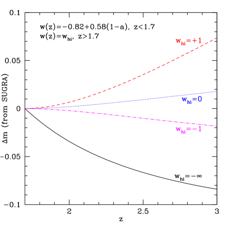
Figure 2: As Fig. 1, but with a fiducial model of SUGRA. This has a less negative equation of state than the cosmological constant (near present observational bounds), giving greater persistence of dark energy density to higher redshifts. Magnitude variations due to $z>1.7$ behavior still remain small, especially in the physically reasonable range $-1\leq w_{\rm hi}\leq 0$.

This demonstrates that even near perfect standard candles in a perfect universe do not motivate precision distance observations for $z>1.7$. As we will show, 1% distance accuracy will be enormously difficult to approach at these high redshifts, due in large part to systematics. Distance markers with greater intrinsic dispersion than SNe Ia, such as gamma ray bursts (which have 1000 times the intrinsic dispersion of SNe Ia (Friedman & Bloom, 2005)), are even less useful. Moreover, both the cosmology and observations have uncertainties and biasing mechanisms. We address some of these in the following sections, beginning with gravitational lensing due to the universe being imperfectly homogeneous.

2.2 Gravitational lensing

As light propagates over longer distances, the source has increased probability of amplification or deamplification due to gravitational scattering (lensing) off large scale structure. Averaged over many sources at a given redshift, the mean flux is unchanged but there is increased dispersion of the source luminosity function. Because the amplification probability distribution is non-Gaussian (skewed toward deamplification), the received flux distribution is also asymmetric and incomplete sampling due to a finite number of sources will impose a bias. This presents a danger in drawing cosmology conclusions from relatively small numbers of high redshift sources, hence affecting gamma ray bursts and gravitational wave sources much more than supernovae. We consider both the dispersion and bias effects.

Holz & Linder (2005) give a rigorous approach to including lensing in cosmological distance measurements. (Note that treating lensing through the matter power spectrum instead of the Monte Carlo method of Holz & Linder (2005) is only a rough approximation and does not incorporate non-Gaussianity or bias.) Their prescription is that for more than $\sim 10$ sources per $0.1z$ interval, the statistics approach Gaussian, the bias is much less than a statistical standard deviation, and the extra dispersion can be treated statistically by adding in quadrature to each supernovae an uncertainty

$$\sigma_{\rm lens}=0.1z/(1+0.07z).$$ (1)

This approximation extends the Holz & Linder (2005) result of $\sigma_{\rm lens}=0.093z$ for dispersion in magnitudes to redshifts $z>2$ (also see Premadi & Martel (2005)).

For the fiducial case of a SNAP-like SN survey, we expect more than a thousand SNe Ia in the range $z=1.7-3$ (see §3.1) so treating lensing as an added dispersion is an excellent approximation, in contrast to cases where there might be only tens of sources in this range. We include lensing effects in this manner for the remainder of this article. Note that out to $z=1.7$, lensing has a small effect for a SNAP-like survey, with less than 5% degradation of cosmological parameter estimation, for SN combined with the distance to the CMB last scattering surface. In §3.5 we consider the tails of the lensing amplification distribution where lensing can cause appreciable (de)magnification, leading to possible confusion between SN types if categorized solely by luminosity. In the next section we examine cosmological bias, due to lensing in part but mostly from misestimation of redshift.

2.3 Redshift errors and bias

The two key quantities entering the distance probe are the flux (as just discussed) and the redshift. An important question is how much the redshift uncertainty degrades the Hubble diagram and cosmological parameter estimation. The great majority of the thousands of SNe discovered at $z>1.7$, especially by a survey dedicated to the follow up of $z\leq 1.7$ events, will lack spectroscopic redshifts. We examine the possibility of photometric redshifts in §3.3; here we investigate the effects in terms of a generic uncertainty $\delta z$.

Propagating redshift uncertainties through even a Fisher matrix approach is nontrivial due to correlations and dependencies. A correct technique would be to include the full covariance matrix ($N_{\rm source}\times N_{\rm source}$) of magnitude errors induced by redshift uncertainties. However, the standard practice in the literature (e.g. Huterer et al. (2004)) is to consider only uncorrelated, Gaussian, redshift bin centroid errors. While Huterer et al. (2004) implement this in terms of new fit parameters, to be marginalized over, we adopt the approach of treating redshift uncertainties as an additional source of dispersion, i.e. approximating the full covariance matrix by diagonal entries. In addition, though, we also consider redshift errors as a systematic effect and, as a function of cosmological parameter bias tolerated, bound the allowed correlated error.

In the statistical approach, the uncertainty $(\partial m/\partial z)\,\delta z$ is added in quadrature with the other magnitude errors. The typical amplitude of the distance modulus contribution to the source magnitude uncertainty is 1.7-0.8 over the range $z=1.7-3$. This is not the full story, however, as the source magnitude must be corrected to the calibrated peak magnitude. The redshift uncertainty also propagates into this through, e.g., the light curve width or stretch correction, which contributes to $m$ a term $\alpha(s-1)$ (Perlmutter et al., 1999). Since the stretch is defined as the observed width $s_{0}$ corrected for time dilation, $s=s_{0}/(1+z)$, then a redshift error gives rise to a magnitude error of $dm=\alpha ds=-\alpha s\,dz/(1+z)$. We adopt the typical SN Ia values of $\alpha=1.5$ and $s=1$.

Figure 3 shows the influence of the photometric redshift statistical uncertainties (and gravitational lensing amplification) on the dark energy equation of state (EOS) determination (as does Fig. 4 for the SUGRA case), assuming a SNAP-like survey extended with 1000 SNe distributed uniformly in $z=1.7-3$. The present value of the EOS is $w_{0}$ and its time variation is measured by $w_{a}=-dw/da|_{z=1}$. First, we see that as mentioned the effects of lensing are small for the canonical SNAP-like SN survey to $z=1.7$. Note that even if the space observations were able to continue detailed, spectroscopic characterization of thousands of SNe Ia out to $z=3$ (note that diffraction limited spectroscopy time increases as $(1+z)^{6}$), with the same systematic error floor of $dm_{\rm sys}=0.02(1+z)/2.7$, the improvement in cosmological parameter estimation is modest.

Next we consider no spectroscopy for SNe Ia in the range $z=1.7-3$, yet somehow keeping the same systematic floor, however adding new systematics from photometric redshift errors. These take the form of random Gaussian uncertainties $\sigma_{\ln(1+z)}$ on the individual source redshifts. Even an uncertainty of 0.05, readily achieved today for $z\lesssim 1$ (Ilbert et al., 2006), brings the cosmology estimation contour most of the way to the ideal case of full spectroscopy. However, the caveat of retaining all other systematics at the same level, without spectroscopic characterization of the SN, is a major obstacle. Even if this were possible, the improvement on extending the distance measurement photometrically to $z=3$ relative to the standard $z=1.7$ survey is only 15% (less than 20% with full spectroscopy). This confirms that the $z=1.7$ depth is well chosen.

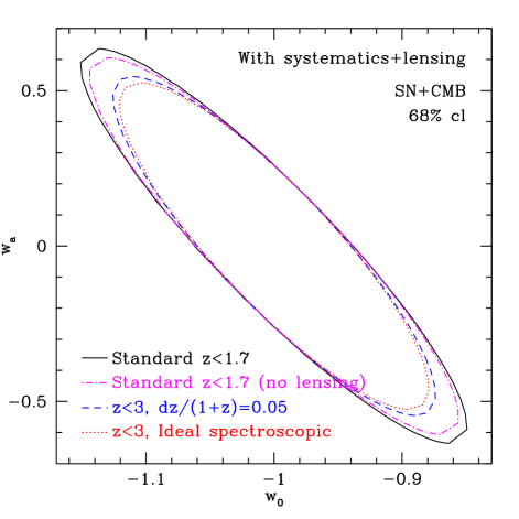
Figure 3: The standard, tightly systematics controlled, $z=1.7$ depth supernova survey is seen to be close to optimal for determination of the dark energy equation of state parameters. Lensing adds less than 5% degradation. Extending the depth to $z=3$, under the ideal case of full spectroscopy and tight systematics control, improves dark energy parameter estimation by less than 20%.

Figure 4: As Fig. 3, for SUGRA dark energy. Due to the model’s greater persistence of dark energy to higher redshift, the improvement of the ideal $z=3$ depth survey relative to the standard $z=1.7$ depth survey can be $\sim 35\%$. However, such persistence may be ruled out by structure growth constraints, e.g. SUGRA deviates by 40% in the matter power spectrum amplitude relative to the cosmological constant case.

A more challenging problem is constraining a systematic component of the photometric redshift errors of the $z>1.7$ SNe, rather than their random scatter. A systematic offset will lead to a bias in cosmological parameter extraction, of more concern than an increased dispersion. Here the redshift error is treated as a coherent systematic shift $\Delta z$ of the derived photometric redshift relative to the true redshift. The resulting bias on a cosmological parameter $p_{i}$ can be obtained through the standard Fisher bias

$$\Delta p_{i}=F^{-1}{}_{ij}\int_{0}^{z_{\rm max}}dz\,N(z)\frac{\partial m}{\partial p_{j}}\Delta m(z)/\sigma_{m}^{2}(z),$$ (2)

where $\Delta m=(dm/dz)\,\Delta z$ is the magnitude offset (including stretch) caused by the redshift systematic $\Delta z$, $\sigma_{m}$ is the overall magnitude dispersion, $N(z)$ is the SN redshift distribution, and $F_{ij}$ is the Fisher matrix.

The bias can be quite pernicious as it can mimic a smooth change in cosmology (see Linder (2006c) for general discussion of biased cosmology). Figure 5 shows the effect of different levels of coherent redshift systematic on cosmological parameter misestimation, for a survey extended to $z=3$. The confidence contours are shifted, biasing the parameters by amounts visible as the difference between the symbols giving the best fit and the heavy x showing the true cosmology. We show 39% confidence level contours so the biases $\Delta w_{0}$ and $\Delta w_{a}$ can be read directly by projecting to the axes.

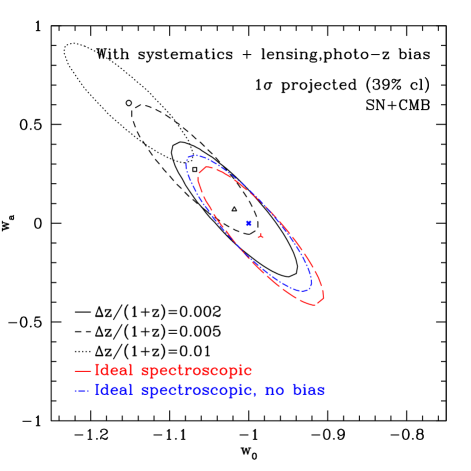
Figure 5: Coherent systematics, such as miscalibrated photometric redshifts or incompletely sampled gravitational lensing amplification, cause bias in cosmological parameter extraction. With many sources, lensing causes a shift of only a small fraction of the statistical uncertainty, from the true cosmology marked with a heavy x to the three legged symbol. Photometric redshift errors can give biases of a substantial fraction of $1\sigma$ (open symbols).

The case labeled “ideal spectroscopic, no bias” shows the contour if one could extend the survey spectroscopically to $z=3$, and unrealistically ignoring lensing bias. The “ideal spectroscopic” (long dashed, red) contour includes the effect of lensing bias. We see that bias from incompletely sampling the lensing amplification distribution is not a major effect, amounting to $<0.2\sigma$ (our sample has about 75 sources per 0.1 redshift bin above $z=1.7$; if we have fewer sources, the bias goes up but so does the statistical uncertainty, so bias is never dominant in the lensing case).

Considering three levels of redshift error, the bias from these can be important, shifting the best fit cosmology by a significant fraction of the statistical uncertainty, as shown by the open symbols. A reasonable fit to the cosmological bias from the propagated redshift error (including stretch) is

$$\frac{\Delta p}{\sigma(p)}\approx 0.2\left(\frac{\Delta z}{1+z}\Big{/}0.001\right),$$ (3)

for $p=w_{0},\,w_{a}$ (the effect is about 2/3 this on $\Omega_{m}$). Thus the photometric redshifts must be calibrated to $\Delta z/(1+z)\lesssim 0.002$ if sources at $z>1.7$ are to be used for cosmology.

While for SUGRA the possible improvement of going from $z=1.7$ to 3 was $\sim$35%, we see that the perils of coherent redshift uncertainties are also more severe (Fig. 6), with parameter biases of 0.26, 0.22, and 0.32$\sigma$ respectively on $w_{a}$, $w_{0}$, and $\Omega_{m}$ per $[\Delta z/(1+z)]/0.001$.

Figure 6: As Fig. 5, for SUGRA dark energy. While the persistence of dark energy density to higher redshifts allows tighter constraint of the cosmological parameters, it also makes them more susceptible to bias from miscalibrated photometric redshifts.

Overall, the random scatter in photo-z’s is not a worry, but possible systematic uncertainties require calibration at the challenging level of 0.002 if the high redshift objects are to give accurate cosmological constraints. Spectroscopy of a thousand $z>1.7$ SN would be quite expensive in time required. In any case, we emphasize that, apart from the numerous pitfalls, standardized candle surveys at $z>1.7$ offer little cosmological leverage on dark energy.

3 Measuring supernovae beyond $z=1.7$

Very high redshift supernovae can be quite interesting for astrophysical issues (which in turn might impact cosmology), to be discussed in §4. Here we consider the measurement aspects of such a sample, and the implementation of observations characterizing the sources, as a practical counterpoint to the theoretical considerations of the previous section.

3.1 Rates

Thousands of supernovae should exist, and be detected by SNAP, at $z>1.7$. See Figure 7 for estimates of both rates; the intrinsic SNe Ia rates are from a fit of observed Supernova Legacy Survey (SNLS: Astier et al. (2006)) rates at $0.3<z<0.8$ (Sullivan et al., 2006b) to the model of Scannapieco & Bildsten (2005). In this model, each of two SN Ia populations has rates proportional either to the star formation rate (SFR) or the total stellar mass. Core-collapse supernova rates are based on HST GOODS rates at $0.3<z<0.7$ (Dahlen et al., 2004) and assume that supernova rates are proportional to the SFR.

We calculate the efficiency of SNAP discovering SNe Ia by assuming a limiting AB magnitude of 28 in each of its nine passbands (Aldering et al., 2004), and a 0.35 magnitude dispersion before correction for light curve shape. We find that SNAP will be almost complete in its discoveries out to $z=3.5$.

For core-collapse supernovae, their heterogeneity and the unknown relative rates of subtypes prevent a meaningful calculation of expected discoveries relative to the total rate shown in Fig. 7. Instead, SNAP itself will furnish unique information on the core-collapse population at high redshift. SNAP’s depth will provide high-redshift core-collapse rates and probe deep into the faint end of their luminosity functions.

The measured rate of core collapse supernovae as a function of redshift will have important implications outside of stellar astrophysics. For one thing, SN feedback is an important ingredient in galaxy formation and properties (e.g. Dekel et al. (1986); Scannapieco et al. (2005)). For another, it determines the spectrum of the SN background in neutrino flux calculations. The Super-Kamiokande detector, once gadolinium trichloride is added to its water, will have excellent sensitivity to the SN background neutrino flux (Beacom & Vagins, 2004). Since the threshold will be $\sim$ 10 MeV (comparable to the average neutrino energy expected from core collapse SNe), the measurable neutrino flux will have contributions from SNe up to $z\mathrel{\raise 1.1625pt\hbox{$<$}\kern-6.99997pt\lower 3.05696pt\hbox{{$\scriptstyle\sim$}}}2$ (Ando & Sato, 2004). A well measured core collapse supernova rate up to high redshifts would thus allow unfolding the average SN energy spectrum (Yueksel, Ando & Beacom, 2005).

Figure 7: The solid and dashed curves show the expected intrinsic observer-frame supernova rates $dN/(dtd\Omega dz)$ of Type Ia and core-collapse supernovae respectively, based on the models discussed in the text. The dot-dashed line is the expected discovery rate of SN Ia with SNAP, adopting an AB=28 limiting magnitude. While uncertainty in the luminosity function precludes a straight-forward prediction of the detectability of the highest redshift core collapse SNe, the SNAP detection threshold should cause a significant roll-over by $z\sim 2-2.5$.

3.2 Light curves

Extracting supernova science from the detected sources requires good characterization of their light curves, or flux vs. time behavior. We calculate the expected signal-to-noise ($S/N$) of the multi-band light curves generated by the “deep” SNAP survey, which repeatedly scans the same sky area, using the SNe Ia spectral template library of Nugent (2005).

Even for a $z=3$ SN Ia that is 0.75 mag fainter than normal, we determine that in the reddest SNAP filter there will be 4 epochs with $S/N>5$ (and many more at a frequency of one point per rest-frame day with slightly lower $S/N$). SNAP will be complete for at least 98% of the unextincted, unlensed supernova luminosity function and essentially complete for $s=1$ SNe Ia. Malmquist bias will be negligible. Section 3.5 discusses the effect of lensing amplification on the SN discovery rate.

From the projected light curve S/N we can estimate how well the SNe Ia distances can be determined. The SNAP filter set consists of nine filters evenly spaced in $\log{\lambda}$ where the effective wavelength of filter $n$ is $\lambda_{n}=(1.16)^{n}\times 4400$Å with $n\in\{0,\dots 8\}$. This spacing, somewhat finer than that of the Johnson-Cousins set, bounds $B$ to $V$-band K-correction uncertainties to less than 0.02 mag (Davis et al., 2006). The supernova-frame $B$-band shifts out of the penultimate $n=7$ filter at $z\gtrsim 1.8$. The low UV flux gives a weak supernova signal in the $n=7$ filter at $z\gtrsim 3$. Thus, color-corrected supernovae at $1.8<z<3$ can be used to measure distances if SNe Ia are standardizable over rest-frame $2500-4000$Å (i.e. around $U$ band).

Whether the $U$-band is useful for determining supernova distances is an open question. Theory suggests that the UV emission is sensitive to metallicity (Domínguez et al., 2001; Lentz et al., 2000). Jha et al. (2006) find that $U$ peak magnitudes are not tightly standardizable, but show a correlation between optical and $U$ light-curve decline rates. Guy et al. (2005) have used published photometry of low-$z$ SNe Ia to establish that $U$-band is stable enough to use for color/extinction corrections. Using the same SN light-curve modeling technique, Astier et al. (2006) show that the $U$ magnitude can be predicted using $B$ and $V$ — to within $\pm 0.03$ magnitude for well-measured SNLS supernovae. In addition high-quality restframe UV spectroscopy of SNLS SNe Ia shows good agreement with that of low-redshift SNe Ia (Sullivan et al., 2006c).

SNAP itself provides UV peak-brightness spectroscopy and light curves of thousands of $z<1.7$ supernovae. If SNe Ia are indeed standardizable in the UV, these data will be used to derive distance-determination algorithms for even higher redshift supernovae. The UV spectral template can be constructed from the subset of objects with measured spectral time-evolution and the supplementary coarse multi-epoch spectroscopy derived from redshift-dependent light-curve shapes. K-corrections and uncertainties for the off-peak photometry necessary for analysis of photometry lacking a corresponding spectrum can be determined as in Nugent et al. (2002); Davis et al. (2006).

Assuming UV standardizability, the SNAP wavelength window provides sufficient coverage to allow extinction corrections of $z>1.7$ supernovae. Based on the expected $S/N$ of $z=2$, 2.5, and 3 supernovae, we calculate the uncertainty in distance modulus $\mu$ obtained from a simultaneous fit of the Cardelli et al. (1989) dust-model parameters $A_{V}$ and $R_{V}$ as well as the supernovae parameters of stretch, peak magnitude, and time of explosion, using the Fisher matrix formalism. For a $z=2$ supernova we find $\sigma(\mu)=0.15$ and 0.05 while fitting for the two- and one-parameter ($R_{V}$ fixed) dust models respectively, compared to the intrinsic dispersion $\sigma_{\rm int}\approx 0.15$. However, for $z=2.5$ these numbers increase to 0.52 and 0.09, while for $z=3$ the two-parameter model is unconstrained, and when $R_{V}$ is fixed to 3.1 then $\sigma(\mu)=0.16$. Uncertainty in the wavelength dependent dust absorption is a major systematic for supernova cosmology. SNAP is specifically designed to control possible dust evolution for SNe at $z<1.7$ by allowing fits of multiparameter dust models. However, SNAP can furnish standardized distances for SNe out to $z=3$ if the dust properties can be adequately constrained.

The expected achievable precision per supernova and the large sample (see §3.1) with high S/N measurements allow determination of the average magnitude in a 0.1 redshift bin to about 0.005 mag. Since the impact on cosmology of an individual bin is small and strongly correlated, one can use bin-to-bin variations to constrain or identify potential systematic effects from K-corrections and photo-z’s.

3.3 Redshift determination

The calculations of §2.3 showed the importance of accurate redshifts for the high-redshift Hubble diagram. In addition, knowledge of redshifts aids in selecting targets for follow-up complementary to that which SNAP will obtain on its own. Here we discuss implementation of such measurements. Obtaining redshifts for such high-redshift SNe will pose a challenge, due to both their faintness and transient nature. Measurement of photometric redshifts of the SN host galaxies can provide an efficient, and possibly necessary, alternative, in combination with calibrating spectroscopic redshifts from the James Webb Space Telescope (JWST) or a thirty meter telescope (generically TMT). We discuss some pros and cons of this and some other possibilities in the remainder of this section.

Supernova host galaxies are expected to have bright luminosities. Even more so than for local SNe Ia the production rate at high redshift should follow the rest-frame $B$ luminosity, and thus the distribution of host galaxy luminosities tracks the luminosity-weighted galaxy luminosity function. The incidence of core-collapse SNe tracks star formation, and star-forming regions have high surface brightness and emit across the full range of SNAP filters. In the SNAP deep field it should be possible to obtain $S/N=10$ photometry for (compact) galaxies as faint as $m_{AB}\sim 29$ at optical/NIR wavelengths (Aldering et al., 2004), corresponding to $M_{B}\sim-18$ at $z=3$. SNAP is thus able to provide precision multi-band photometry covering the spectral features necessary for photometric redshift determination of a large fraction of supernova hosts out to $z=3$.

Detection of the 4000Å break will be possible to $z\sim 3$ with the SNAP filter set for sufficiently luminous host galaxies possessing significant old stellar populations. Galaxies that would evolve into present day ellipticals would have blue spectra at $z\sim 3$ resembling those of present-day Sb galaxies, so the 4000Å break will be present in many galaxies. In these cases there is no redshift determination bias introduced a priori since this feature is stable and carries the most weight in redshift estimation. For starburst galaxies, spectral features are much more subtle (Shapley et al., 2003; Abraham et al., 2004) and the continuum shape, which is affected by extinction, the stellar IMF, and IGM absorption, has relatively more weight. This generally leads to larger scatter in photometric redshifts, and may make photometric redshifts for starburst galaxies more prone to bias. (Redshifts of $1.7<z<3$ starbursts could be better constrained with the help of deep ground-based $U$-band observations of the SNAP deep field.)

Spectroscopic redshifts are required to accurately calibrate SNAP photometric redshifts. The accuracy of SNAP photometric redshifts of galaxies during the mission should be sufficient to allow reliable selection of SNAP transients for complementary follow-up studies (Aldering et al., 2004; Dahlen, 2006). The final set of precise photometric redshift calibration necessary for cosmological analysis would not be needed until SNAP observations are well underway. Even for photometric redshifts with scatter at very high redshift of $\sigma_{\ln(1+z)}\sim 0.05$, one thousand calibration spectra could achieve the level $\Delta z/(1+z)\sim 0.002$ needed to use SNe Ia with $z>1.7$ for unbiased cosmology (see §2.3). (Recall that for $z<1.7$, $\partial m/\partial z$ is larger and significantly more stringent redshift determination is required.)

The necessary calibration reaching to the photometric redshift limit of SNAP is probably tractable with multi-slit spectroscopy of galaxies in the SNAP deep field using JWST or TMT. The surface density of galaxies in the SNAP deep field will be of order 250 arcmin^-2 (Aldering et al., 2004), allowing for efficient multi-object spectroscopy. At optical wavelengths TMT could easily obtain redshifts to $m_{AB}=26$ for a few thousand galaxies per night; this would be sufficient to calibrate the brighter star-forming galaxies. For the oldest — UV-faint — galaxies, near infrared (NIR) spectroscopy with NIRspec on JWST might be necessary. Self-contained spectroscopy of galaxies which land “for free” in the SNAP IFU spectrograph — obtained in parallel with SNAP imaging observations — also provides some calibration of photometric redshifts. NIRspec on JWST would require 30 hours to reach $S/N\sim 10$ per resolution element for m${}_{AB}\sim 28$ galaxies with $R\sim 100$, and would be able to observe $\sim 100$ objects simultaneously at NIR wavelengths (Jakobsen et al., 2005). TMT would require of order 80 hrs to reach comparable $S/N$ to m${}_{AB}\sim 28$ at optical wavelengths, with $\sim 500$ galaxies observed at once. Multi-week campaigns on these facilities would be necessary to achieve sample sizes of order 1000 galaxies with m${}_{AB}\sim 28$. Note that follow-up of the SNAP deep fields is likely to be of major interest for, e.g., JWST and TMT, independent of a need for photometric redshift calibration.

The efficacy of measuring photometric redshifts from the supernovae themselves depends heavily on SN physical properties. Type Ia supernova light curves, due to their phase-dependent color evolution and sensitivity to broad spectral features, enable photometric determination of redshifts. Current algorithms and templates applied to the SNLS dataset predict photometric redshifts for which 90% of SNe Ia deviate by $\mathrel{\raise 1.1625pt\hbox{$<$}\kern-6.99997pt\lower 3.05696pt\hbox{{$\scriptstyle\sim$}}}0.08$ and the median absolute error is 0.03 when compared to spectroscopically measured redshifts (Sullivan et al., 2006a). Next generation telescope surveys with more filters and higher $S/N$ should yield further improvement.

The precision and accuracy that supernova photometric redshifts can achieve are limited, however. Complications could arise if the SN photospheric velocity, which decreases as the light curve brightens and fades, were to change systematically with redshift. As shown in §2.3, a photometric redshift bias no larger than 0.002 can be tolerated for $z>1.7$ cosmological measurements. This translates into a maximum allowable shift in the ensemble photospheric velocity — potentially introduced by sample selection biases or intrinsic changes in SNe Ia — of 600 km/s. The scatter amongst SNe Ia at a given phase is $\sim 1300$ km/s (Benetti et al., 2005). Hence the ensemble velocity need only shift by less than half the observed scatter in order to greatly impact cosmological measurements at such high redshift. Thus external constraints on expansion velocity evolution, e.g. up to $z=1.7$ from the SNAP spectrograph, will be needed to assess the efficacy of using photometric redshifts from the SNe Ia themselves for cosmology.

As described above, calibrated photometric redshifts from the host galaxies are sufficient to satisfy the bias limit for the redshift range $z>1.7$. Independently determined photometric redshifts from the SN lightcurves could then play a role in resolving remaining ambiguities. The accuracy of the photometric redshifts is certainly sufficient for triggering targeted follow-up programs, e.g. using JWST.

3.4 Supernova typing

Categorizing the supernovae into types is an essential element of supernova, astrophysical, and cosmological studies. Photometric segregation of supernovae can be performed with some success based on lightcurve and color evolution. Early variations of this approach have been presented in Poznanski et al. (2002); Gal-Yam et al. (2004); Riess et al. (2004); Barris & Tonry (2004). In general, when restframe UV data are available Type II SNe are seen to be UV-bright whereas opacity from iron-group elements in SNe Ia suppresses the UV brightness. In addition, the lightcurves of SNe IIP are quite distinct from those of other SN types. Using a Monte Carlo lightcurve simulation appropriate to the color coverage, cadence, and depth of SNAP we confirm that for the $S/N$ achievable for SNe Ia at $z=3$ the shape of the B-band lightcurve distinguishes between Type Ia and Type IIP SNe.

Distinguishing Types Ib and Ic from Type Ia is more difficult, especially in the face of an uncertain redshift and dust extinction. SNe Ib/c are generally redder than SNe Ia (with restframe B-V color about 0.5 magnitudes redder (Poznanski et al., 2002)). The color evolution is different as well: Type Ib/c have similar pre- and post-maximum colors while Type Ia become redder after their maximum brightness is reached. The colors and magnitude can be used to largely break the degeneracy between dust reddening and SN type once a full lightcurve is obtained. The precise multi-band photometry afforded by SNAP can greatly improve the power of such techniques.

The largest and most complete sample on which this technique has been tested to date is the Supernova Legacy Survey. Sullivan et al. (2006a) use 4-color lightcurve photometry to reject all ten SNe II while rejecting only one SN Ia in a sample of 85 spectroscopically-classified high-redshift SNe. However, Sullivan et al. (2006a) do not demonstrate their ability to reject SNe Ib/c and they do not comment on whether or not all the SNe II were IIP, or might have included SNe IIL.

At the redshifts $z>1.7$ considered here, all stellar populations will be young, and therefore galaxy morphology based shortcuts applicable at lower redshift, e.g. that ellipticals never host core-collapse SNe, cannot be used. With the spatial resolution (e.g. 1 kpc at $z=3$) and multicolor information from SNAP it may be possible to sufficiently constrain the stellar population age at the (projected) location of a SN to partly discriminate some core-collapse SNe from SNe Ia. The critical assumption here is that most core-collapse SNe will be produced in regions dominated by a single starburst, and that the light of such a starburst will have high surface brightness and thus dominate over any underlying older population. In this case multicolor photometry covering the restframe UV can constrain the starburst age and therefore the lowest mass of the stars completing their evolution. Taking $8~{}M_{\odot}$ as the dividing line between core-collapse and thermonuclear supernovae (Iben & Renzini, 1983), evidence of a starburst younger than 50 Myr (Schaller et al., 1992; Schaerer et al., 1993) at the location of a SN would strongly suggest that the SN is a core-collapse SN. Protracted starbursts, low-level star formation, and projection effects will complicate this technique. Absence of detectable star formation anywhere near a SN would suggest a SN Ia, but it will be difficult to rule-out low-level star formation and hence a core-collapse origin. Again, SNAP spectroscopic follow-up of SNe hosts at lower redshift will help calibrate this technique.

Detection of the shock breakout from core-collapse SNe would provide a completely new and independent means of discriminating SN types. As discussed in §4.3, predictions of luminosity and timescale, and hence detectability, are quite uncertain. It is encouraging in this respect that shock breakout has been detected at restframe optical wavelengths in low redshift Type II (SN 1987A, Menzies et al. (1987); Hamuy et al. (1988)), IIb (SN 1993J, Lewis et al. (1994); Richmond et al. (1994)), and Ib/c (SN 1999ex, Stritzinger et al. (2002)) SNe with timescales and luminosities that SNAP could detect out to high redshift. SNAP will sample the restframe UV of high-redshift SNe, where the hot shock breakout will be brighter, however, the fastest events may be missed due to SNAP’s 1-2 day restframe cadence.

It is tempting to exploit the fact that core-collapse SNe are generally fainter at peak than SNe Ia to obtain the type. However, the luminosity functions do overlap (Richardson et al., 2002, 2006), and gravitational lensing (see the next section), extinction, and redshift errors can further blur this distinction. Using luminosity as the sole type discriminant would surely bias any cosmological measurement by modifying the statistical distribution of true SNe Ia and inviting interlopers (Homeier, 2005). Luminosity still may prove useful as a weak prior in concert with other type discriminants. Without the need to trigger spectroscopic followup, one can wait for the full light curve to type the supernova. The magnitude might, however, be used to feed the supernova to JWST or TMT; this poses no danger as that spectroscopic information will confirm the type.

3.5 Typing and lensing amplification

Gravitational lensing can confuse typing through both amplification and deamplification of the intrinsic luminosity. While SN Ib/c have a wider intrinsic dispersion than Ia, typically they are 1-2.5 magnitudes fainter. The probability of SN Ib/c being sufficiently strongly amplified by lensing to reach Ia luminosity is small, and likely would be accompanied by multiple images or other signs that lensing is present.

We can assess the converse process – Ia being demagnified by 1 mag – through looking at the maximum demagnification possible as a function of redshift. Since magnification is dominated by the Ricci focusing of light by density inhomogeneities, and one cannot have an underdensity with density less than zero, then the maximum demagnification is determined by the empty beam distance $d_{\rm empty}$ where all matter is removed from the line of sight. The distance-redshift relation for arbitrary clumpiness (over- or underdensity) and arbitrary dark energy equation of state was derived by Linder (1988). The demagnification is then bounded by $\Delta m<5\log(d_{\rm empty}/d)$, where $d$ is usual Friedmann-Robertson-Walker luminosity distance.

Figure 8 shows that for $z<3$ the demagnification is less than 0.7 mag and hence SNe Ia are only likely to overlap with the bright tail of the SNe Ib/c luminosity function in the most extreme empty beam case, and only at the highest redshifts. A fitting formula valid to better than 0.01 mag out to $z=4$ for the maximum demagnification in a dark energy cosmology is given by

$$\Delta m = Az^{2},\quad z<1$$ (4)

$$= A+1.93A(z-1),\quad z\geq 1$$ (5)

where $A=0.14-0.04[1+w(z=1)]$.

Figure 8: The maximum demagnification is given by difference between apparent magnitude in an empty beam model (zero matter along the line of sight) and a smooth, FRW model. The curves show the results for two different dark energy models.

3.6 Using lensed high redshift supernovae

In addition to acting as noise, causing dispersion and bias, gravitational lensing also provides an astrophysically useful signal. The extension of Eq. (1) to high redshift contains important information on structure formation. The dispersion as a function of depth can provide constraints on the mass amplitude $\sigma_{8}$ and the evolution of the matter power spectrum (Frieman, 1997; Dodelson & Vallinotto, 2005), while the cosmic variance along different lines of sight also carries valuable knowledge of the matter distribution (Pen, 2004; Cooray et al., 2006).

Individual, strongly lensed standardized candles, as well as their statistics, provide important probes of cosmology and galaxy cluster mass profiles and velocity dispersions through the amplification time variation, multiple image separations, image flux ratios, and time delays (Holz, 2001; Goobar et al., 2002; Lewis & Ibata, 2002; Linder, 2004). The high quality, multiband, cadenced sample of tens of strongly lensed, very high redshift supernovae from SNAP will contribute a rich science resource.

4 Astrophysics and systematics

Very high redshift supernovae open windows on several areas of astrophysics. We examine here the use of such observations to learn about supernova physics and dust properties.

4.1 Progenitor and environmental systematics

The study of supernovae at high redshifts offers the possibility of seeing evolutionary effects in action. SNAP will exploit this feature extensively to decouple systematics from the true cosmological signal using its $z<1.7$ sample. Given the relative insensitivity of luminosity distance to dark energy for $z>1.7$ (see §2.1), deviations in the Hubble diagram could potentially be useful as a means to reveal astrophysical systematics (Riess & Livio, 2006). The value of such higher redshift SNe Ia for probing systematics that could affect cosmological measurements thus hinges on whether or not some property of SNe Ia is especially-well probed or constrained in this redshift interval. Such circumstances might include extraordinarily low metallicity or extension of the lookback time early enough such that the upper limit set by the age of the universe meaningfully constrains the timescales for SN Ia progenitor models.

In reality, extending the study of SNe Ia from $z=1.7$ to $z=3$ increases the lookback time by a mere 1.7 Gyr. Since the age for a $\Omega_{m}=0.3$, flat $\Lambda$CDM universe at $z=3$ is 2.2 Gyr, the first generations of stars in the canonical 3–8 $M_{\odot}$ mass range expected for C/O white dwarf progenitors (Iben & Renzini, 1983) will have evolved and begun producing SNe Ia via the various channels currently in contention (Belczynski et al., 2005). Therefore, it will remain difficult to directly probe systematic effects due to the progenitor mass. Even proposed channels with long delay times of 2–4 Gyr (Strolger et al., 2004; Scannapieco & Bildsten, 2005) would be operative over the $1.7<z<3$ redshift range. Therefore, in order to distinguish between progenitor scenarios, detailed modeling of star formation histories, binary parameters, etc., for various progenitor scenarios will be required just as it is for the $z<1.7$ SN Ia population (e.g. Förster et al., 2006).

Similarly, one cannot expect SNe Ia progenitors to be dominated by low-metallicity systems. Most of the gas that assembles into stars that will explode as SNe Ia at $1.7<z<3$ will be enriched with metals, as the most massive galaxies are already in place by $z\sim 3$ (Steidel et al., 1996; Heavens et al., 2004; van Dokkum et al., 2006). Even the lower-density, lower SN-yield, environments probed by damped Lyman-$\alpha$ absorbers are enriched. This can be seen directly from [Zn/H] measurements of damped Lyman alpha systems (DLAs) (Prochaska et al., 2003; Kulkarni et al., 2005), which show $-0.4<{\rm[Fe/H]}<-2.5$ over the range $1.7<z<4$. This is despite the fact that DLAs will exhibit lower metallicity than the average due to several selection effects, including the preferential selection of outer regions of the galaxies associated with the DLAs, metallicity gradients in galaxies, the upper limit on $N_{HI}$ included in the definition of DLAs, etc. (Zwaan et al., 2005; Johansson & Efstathiou, 2006). This range in DLA metallicity is not that much larger than that found amongst nearby galaxies.

Determining the evolution timescale(s) is important for understanding the allowed combinations of binary systems leading to the creation of SNe Ia. The ideal laboratory for such studies is a delta-function episode of star-formation, since then the starting time is defined. In reality one must deal with finite star-formation timescales, either within specific galaxies or across all galaxies. The rising global SFR at $z\sim 3$ (Hopkins & Beacom, 2006) means that those progenitor systems formed at much higher redshift with potentially much lower metallicity and having a long delay time will be overwhelmed in numbers by younger progenitors having lower delay times. Conversely, the dramatic roll-over of the global SFR for galaxies at $z<1$ (Heavens et al., 2004; Juneau et al., 2005; Hopkins & Beacom, 2006) may make this redshift range the most useful in revealing details of a progenitor population having a long delay time.

Important effects, especially those related to metallicity, may still be revealed. For instance modeling by Domínguez et al. (2001) and Lentz et al. (2000) suggest that changes in progenitor metallicity will affect the metallicity of the ejecta composition, and thus its opacity and brightness in the UV. On the other hand, Kobayashi et al. (1998) have suggested that the production of SNe Ia will be inhibited as the metallicity of the gas from the donor star decreases, choking-off around [Fe/H] $\sim-1$. The broad ramification of this model for cosmology is that SNe Ia from [Fe/H] $<-1$ progenitors will not exist, and therefore metallicity-dependent effects will be truncated. Indeed, as metallicity correlates much more strongly with galaxy luminosity than with redshift, metallicity-dependent systematics studies from higher redshift SNe Ia may be secondary to what can be learned by the study of SNe Ia in local galaxies (Hamuy et al., 2000; Gallagher et al., 2005).

In the simple galaxy chemical evolution models presented by Kobayashi et al. (1998), the SN Ia rate would plummet around $z\sim 1.2$, where the galaxy metallicity crosses the [Fe/H] $\sim-1$ threshold. In reality the redshift at which a galaxy passes the [Fe/H] $\sim-1$ threshold will be mass-dependent, and environmental affects on galaxy star formation histories will further blur the [Fe/H] $\sim-1$ threshold in redshift space. Therefore, what may be observed is a gradual drop in the SNe Ia rate, superimposed on the modulation already expected due to the SFR, that could well continue to $z\sim 3$. As galaxy metallicities at $z\sim 3$ will be difficult to obtain directly (e.g. Shapley et al. (2005)), modeling of this effect will be strongly coupled to galaxy formation and SF models.

It is also possible that extremely low metallicity environments (Jimenez & Haiman, 2006), will lead to so-called “Type 1.5” SNe, in which the C/O core of an AGB star reaches the Chandrasekhar limit (Iben & Renzini, 1983). For instance, Tsujimoto & Shigeyama (2006) has proposed that ultra-metal-poor stars, with [Fe/H] $<-5$ will produce SNe 1.5. It may be possible that stars up to [Fe/H] $\sim-1$ can produce SNe 1.5, e.g., if the mass loss from stellar winds decreases sufficiently with decreasing metallicity (Zijlstra, 2004). These events would be hydrogen rich, possibly similar to SN 2002ic (Wood-Vasey, 2002; Hamuy et al., 2003; Wood-Vasey et al., 2004) or SN 2005gj (Prieto et al., 2005; Aldering et al., 2006). The potential of such SNe as standard candles has yet to be explored.

All things considered, typical $1.7<z<3$ SNe Ia may not probe a fundamentally different region of parameter space than those at $z<1.7$. Of course it is still possible that individual SNe Ia, e.g. in an ultra-low metallicity or very young environment, will offer important clues to understanding SNe Ia. For these, higher $S/N$ photometry extending to longer wavelengths, as well as spectroscopy, would be very valuable. In these cases JWST could be employed if the uniqueness of such SNe can be realized in time from SNAP observations to trigger dedicated follow-up. Meanwhile, local SN observations are rapidly expanding efforts to probe young stellar populations in low metallicity environments (Wood-Vasey et al., 2004; Aldering et al., 2006), as well as continuing the unique study of SNe Ia in old and/or metal-rich stellar populations possible at low redshift.

4.2 Extinction and dust properties

Accurate extinction measurements are necessary for the cosmological use of supernovae as standard candles. Alternatively, we can view supernovae as providing a source with known spectral energy distribution by which we can constrain the extinction properties of dust. This also allows tests of the applicability of the Cardelli et al. (1989) extinction model at observed SN-frame wavelengths (as discussed in §3.2, SNe Ia standardizability in the UV can be tested with SNAP data itself). Beyond this, a foundation for models of extinction wavelength-dependence may be laid by study of the subset of $z<1$ SNe II caught at shock breakout, through deviations from fixed blackbody color at the Rayleigh-Jeans tail (see §4.3). Additionally, strongly lensed quasars in the SNAP fields provide differential extinction on different lines of sight (Falco et al. (1999), but see McGough et al. (2005)).

SNAP observation of supernovae at $z>1.7$ furnishes information on dust extinction in the UV. Together with supplemental JWST followup, we can have measurements of UV-optical or optical-NIR extinction along many supernova lines of sight. This extends such astrophysical dust studies over the great majority of the age of the universe.

One final challenge will be absorption from the intergalactic medium. Simulations (Madau, 1995; Meiksin, 2006) and observations (Songaila, 2004) indicate observer-frame $B$-band absorption of $\sim 0.1$ mag by $z=2.5$ and 0.3-0.4 mag by $z=3$, largely from hydrogen. Likewise, observer-frame $V$-band absorption is expected to be $\sim 0.1$ mag by $z=3$. Longer wavelengths relevant for high-redshift SNe Ia will not be affected by hydrogen, but the UV spectra of the brightest SNe II will be affected. Metal lines could in principle affect longer wavelengths in certain filters, depending on the sightline. But on average they should cause absorption well below 0.01 mag (Songaila, 2005). For SNe seen through DLA systems broadband extinction may not be negligible (Ellison et al., 2005; York et al., 2006).

4.3 Shock breakout in core collapse SNe

Core collapse SNe exhibit the signature phenomenon of shock breakout (Colgate, 1968) when the forward shock reaches the stellar surface. Observation of this event would help type the SN and carries potentially valuable information on the physical properties of the progenitor. The characteristic timescale of the shock breakout depends on the structure of the progenitor star, with compact blue supergiants (BSG) expected to produce shocks with cosmological restframe timescales of 0.03 hrs, compared to 0.3 hrs for the much more extended red supergiants (RSG) (Matzner & McKee, 1999). These values for all but the largest stars will be affected by the light travel time across the star (Ensman & Burrows, 1992). Both progenitor types are expected to produce peak shock temperatures in the range $T\sim 0.5-1\times 10^{6}$ K and peak luminosities of $L\sim 10^{45}$ erg s^-1. While this emission peaks at soft X-ray wavelengths, there can be significant emission in the restframe UV wavelengths that SNAP will sample. Moreover, the timescale for strong emission in the UV can range from a significant fraction of a day to several days (Ensman & Burrows, 1992; Young et al., 1995; Blinnikov et al., 1998, 2000).

There exist four examples of low-redshift core-collapse SNe to date where detection of shock breakout is certain (SN 1987A, SN 1993J, and SN 1999ex) or probable (GRB 060218/ SN 2006aj; for this case there is concern that the emission is not necessarily all from classical shock breakout). To our knowledge, these also constitute the full sample of core-collapse SNe discovered within a day or two of explosion, but we caution that still it is possible that they are not representative. Restframe U-band observations of these events indicate approximate un-dereddened absolute AB magnitudes greater than $-15.3$, $-19.5$, $-14.7$ for SN 1987A, SN 1993J, and SN 1999ex, respectively, and equal to $-18.2$ for GRB 060218/SN 2006aj during the shock breakout phase (Moreno & Walker, 1987; Menzies et al., 1987; Hamuy et al., 1988; Lewis et al., 1994; Richmond et al., 1994; Stritzinger et al., 2002; Campana, 2006). (The lower limits reflect the fact that the peak of shock breakout emission in $U$-band was missed in most cases.) Perhaps more relevant for typing purposes is that for all cases except SN 1999ex, the shock breakout phase was the brightest epoch of the $U$-band lightcurve. Thus, if SNAP detects a core-collapse SN, it appears likely that it will also be sensitive to the shock breakout.

As SNAP will sample further into the restframe UV — down to restframe Ly-$\alpha$ in its bluest bands, detections should be somewhat stronger, depending on the amount of dust extinction. For example at restframe 1800 Å, GRB 060218/SN 2006aj exhibited an absolute AB magnitude of $-18.4$ (Campana, 2006). The shock breakout for SN 1993J, having a RSG progenitor (Aldering et al., 1994; Van Dyk et al., 2002), is one example that SNAP should be capable of detecting out to $z\sim 3$.

SNAP samples any given patch of sky with 4 exposures of 300 sec in each of the bluest (optical) filters and with 8 exposures of 300 sec in each of the reddest (NIR) filters. Consecutive observations in each of the 9 SNAP filters means that a given patch of sky is monitored continuously for 1.1 hrs every 4 days in the observer frame. Thus, with fortuitous timing — likely for some fraction of the thousands of core-collapse SNe SNAP will detect — SNAP may obtain multi-epoch coverage in up to 9 filters, possibly covering the most luminous period of an event even for fast-declining BSG progenitors. This will allow a determination of the luminosity and temperature (spectral) evolution of the shock breakout. In simple shock breakout models (Matzner & McKee, 1999) this evolution is set primarily by the stellar radius, followed in importance by the explosion energy, and finally the total ejecta mass. Determinations of the redshift and dust extinction will be needed to set the correct scale for these quantities for each SN. Some common physical parameters (such as opacities — expected to be dominated by electron scattering — and characteristic density profiles) will need to be determined for the population as a whole in order obtain the best constraints (Matzner & McKee, 1999; Calzavara & Matzner, 2004). However, distinguishing between BSG and RSG progenitors for shock breakout events with good temporal coverage should be straightforward, and this discrimination is already sufficient to provide more detailed constraints on the star formation history of the universe than can be obtained from the integrated light of galaxies or from SN rates alone.

5 Conclusions

As part of its normal operation SNAP will discover and obtain lightcurves for thousands of SNe with $z>1.7$. For SNe Ia, we find that SNAP will have good sensitivity out to $z\sim 3$, where the nominal 4-day observer-frame cadence will equal an unprecedented daily cadence in the rest-frame.

However, we find that attempting to use $z>1.7$ standardized candles for cosmology leads to weak statistical gains and is prone to new systematic errors – a high risk, low yield strategy that undoes the careful systematics control SNAP provides at $z<1.7$. We conclude that in the case of SNe Ia, limited wavelength coverage, and lack of SN and host spectroscopy, would additionally open the door to biases in redshift, contamination from SNe IIL and Ib/c, and poorer standardizability due to dust and metallicity in the rest-frame UV. These observational issues could be remedied in principle with supporting JWST spectroscopy and rest-frame optical lightcurves. Largely due to overhead, SNAP-quality follow-up of even 100 SNe Ia in the range $1.7<z<3$ with JWST would constitute a very large program, and attaining SNAP-level calibration might also be an issue.

While the utility of such SNe Ia appears marginal for precision measurements of the cosmological parameters, such SNe — both thermonuclear and core collapse — will be valuable for understanding many aspects of stellar and galaxy evolution. The core collapse SNe will further help in understanding the neutrino background. JWST follow-up of the most unusual SNe, including lensed SNe, could also prove useful — for general astrophysical problems, and perhaps for dark matter and cosmological measurements.

References

- Abraham et al. (2004) Abraham, R. G., et al. 2004, AJ, 127, 2455
- Aldering et al. (1994) Aldering, G., Humphreys, R. M., & Richmond, M. 1994, AJ, 107, 662
- Aldering et al. (2004) Aldering, G., & the SNAP collaboration 2004, astro-ph/0405232
- Aldering et al. (2006) Aldering, G., & the SNfactory collaboration 2006, ApJ, accepted astro-ph/0606499
- Ando & Sato (2004) Ando, S., & Sato, K. 2004, New Journal of Physics, 6, 170
- Astier et al. (2006) Astier, P. et al. 2006, A&A, 447, 31
- Barris & Tonry (2004) Barris, B. J., & Tonry, J. L. 2004, ApJ, 613, L21
- Beacom & Vagins (2004) Beacom, J. F., & Vagins, M. R. 2004, Physical Review Letters, 93, 171101
- Belczynski et al. (2005) Belczynski, K., Bulik, T., & Ruiter, A. J. 2005, ApJ, 629, 915
- Blinnikov et al. (1998) Blinnikov, S. I., Eastman, R., Bartunov, O. S., Popolitov, V. A., & Woosley, S. E. 1998, ApJ, 496, 454
- Blinnikov et al. (2000) Blinnikov, S., Lundqvist, P., Bartunov, O., Nomoto, K., & Iwamoto, K. 2000, ApJ, 532, 1132
- Benetti et al. (2005) Benetti, S., et al. 2005, ApJ, 623, 1011
- Calzavara & Matzner (2004) Calzavara, A. J., & Matzner, C. D. 2004, MNRAS, 351, 694
- Campana (2006) Campana, S. 2006, Nature, accepted, (astro-ph/0603279)
- Cardelli et al. (1989) Cardelli, J. A., Clayton, G. C., & Mathis, J. S. 1989, ApJ, 345, 245
- Colgate (1968) Colgate, S. A. 1968, Canadian J. Phys. 46, 476.
- Cooray et al. (2006) Cooray, A., Holz, D., & Huterer, D. 2006, ApJ, 637, L77
- Dahlen et al. (2004) Dahlen, T., et al. 2004, ApJ, 613, 189
- Dahlen (2006) Dahlen, T., http://www.physto.se/~dahlen/PhotozSNAP.html
- Davis et al. (2006) Davis, T. M., Schmidt, B. P., & Kim, A. G. 2006, PASP, 118, 205
- Dekel et al. (1986) Dekel, A. & Silk, J. 1986, ApJ, 303, 39
- Dodelson & Vallinotto (2005) Dodelson, S. & Vallinotto, A., astro-ph/0511086
- van Dokkum et al. (2006) van Dokkum, P. G., et al. 2006, ApJ, 638, L59
- Domínguez et al. (2001) Domínguez, I., Höflich, P., & Straniero, O. 2001, ApJ, 557, 279
- Ellison et al. (2005) Ellison, S. L., Hall, P. B., & Lira, P. 2005, AJ, 130, 1345
- Ensman & Burrows (1992) Ensman, L., & Burrows, A. 1992, ApJ, 393, 742
- Falco et al. (1999) Falco, E. E., et al. 1999, ApJ, 523, 617
- Förster et al. (2006) Förster, F., Wolf, C., Podsiadlowski, P., & Han, Z. 2006, MNRAS, 397 .
- Friedman & Bloom (2005) Friedman, A. S. & Bloom, J. S. 2005, ApJ, 627, 1.
- Frieman (1997) Frieman, J. A. 1997, Comments Astrophys. 18, 323
- Gallagher et al. (2005) Gallagher, J. S., Garnavich, P. M., Berlind, P., Challis, P., Jha, S., & Kirshner, R. P. 2005, ApJ, 634, 210
- Gal-Yam et al. (2004) Gal-Yam, A., Poznanski, D., Maoz, D., Filippenko, A. V., & Foley, R. J. 2004, PASP, 116, 597
- Goobar et al. (2002) Goobar, A., Mortsell, E., Amanullah, R., Nugent, P., A&A, 393, 25
- Guy et al. (2005) Guy, J., Astier, P., Nobili, S., Regnault, N., & Pain, R. 2005, A&A, 443, 781
- Hamuy et al. (1988) Hamuy, M., Suntzeff, N. B., Gonzalez, R., & Martin, G. 1988, AJ, 95, 63
- Hamuy et al. (2000) Hamuy, M., Trager, S. C., Pinto, P. A., Phillips, M. M., Schommer, R. A., Ivanov, V., & Suntzeff, N. B. 2000, AJ, 120, 1479
- Hamuy et al. (2003) Hamuy, M., Phillips, M. M., Suntzeff, N. B., Maza, J., Gonzalez, L. E., Roth, M., Krisciunas, K., Morrell, N., Green, E. M., Persson, S. E., & McCarthy, P. J. 2003, Nature, 424, 651
- Heavens et al. (2004) Heavens, A., Panter, B., Jimenez, R., & Dunlop, J. 2004, Nature, 428, 625
- Holz (2001) Holz, D. E. 2001, ApJ, 556, L71
- Holz & Linder (2005) Holz, D. E. & Linder, E. V. 2005, ApJ, 631, 678
- Homeier (2005) Homeier, N. L. 2005, ApJ, 620, 12
- Hopkins & Beacom (2006) Hopkins, A. M. & Beacom, J. F. 2006, ApJ, accepted, astro-ph/0601463
- Huterer et al. (2004) Huterer, D., Kim, A., Krauss, L.M., Broderick, T. 2004, ApJ, 615, 595
- Iben & Renzini (1983) Iben, I., & Renzini, A. 1983, ARA&A, 21, 271
- Ilbert et al. (2006) Ilbert, O., et al. 2006, astro-ph/0603217
- Jakobsen et al. (2005) Jakobsen, P., et al. 2005, BAAS, 207
- Jha et al. (2006) Jha, S., et al. 2006, AJ, 131, 527
- Jimenez & Haiman (2006) Jimenez, R., & Haiman, Z. 2006, Nature, 440, 501
- Johansson & Efstathiou (2006) Johansson, P. H., & Efstathiou, G. 2006, astro-ph/0603663
- Juneau et al. (2005) Juneau, S., et al. 2005, ApJ, 619, L135
- Kim & Miquel (2006) Kim, A.G. & Miquel, R. 2006, Astropart. Phys. 24, 451
- Knop et al. (2003) Knop, R. A., et al. 2003, ApJ, 598, 102
- Kobayashi et al. (1998) Kobayashi, C., Tsujimoto, T., Nomoto, K., Hachisu, I., & Kato, M. 1998, ApJ, 503, L155
- Kulkarni et al. (2005) Kulkarni, V. P., Fall, S. M., Lauroesch, J. T., York, D. G., Welty, D. E., Khare, P., & Truran, J. W. 2005, ApJ, 618, 68
- Lentz et al. (2000) Lentz, E. J., Baron, E., Branch, D., Hauschildt, P. H., & Nugent, P. E. 2000, ApJ, 530, 966
- Lewis & Ibata (2002) Lewis, G. F, & Ibata, R. A. 2002, MNRAS, 337, 26
- Lewis et al. (1994) Lewis, J. R., et al. 1994, MNRAS, 266, L27
- Linder (1988) Linder, E. V. 1988, A&A, 206, 190
- Linder & Huterer (2003) Linder, E. V. & Huterer, D. 2003, Phys. Rev. D 67, 081303
- Linder (2004) Linder, E. V. 2004, Phys. Rev. D 70, 043534
- Linder (2006a) Linder, E. V. 2006a, Astroparticle Physics, 25, 167
- Linder (2006b) Linder, E. V. 2006b, Astroparticle Physics, accepted (astro-ph/0603584)
- Linder (2006c) Linder, E. V. 2006c, Astroparticle Physics, accepted (astro-ph/0604280)
- Madau (1995) Madau, P. 1995, ApJ, 441, 18
- Matzner & McKee (1999) Matzner, C. D., & McKee, C. F. 1999, ApJ, 510, 379
- McGough et al. (2005) McGough, C., Clayton, G. C., Gordon, K. D., & Wolff, M. J. 2005, ApJ, 624, 118
- Meiksin (2006) Meiksin, A. 2006, MNRAS, 365, 807
- Menzies et al. (1987) Menzies, J. W., et al. 1987, MNRAS, 227, 39P
- Moreno & Walker (1987) Moreno, B., & Walker, S. 1987, IAU Circ., 4316, 1
- Neill et al. (2006) Neill, J. D., et al. 2006, astro-ph/0605148
- Nugent et al. (2002) Nugent, P., Kim, A., & Perlmutter, S. 2002, PASP, 114, 803
- Nugent (2005) Nugent, P. 2005, http://supernova.lbl.gov/~nugent/nugent_templates.html
- Oguri & Takahashi (2006) Oguri, M. & Takahashi, K. 2006, Phys. Rev. D, accepted, astro-ph/0604476
- Pen (2004) Pen, U-L. 2004, New Astron. 9, 417
- Perlmutter et al. (1999) Perlmutter, S. et al. 1999, ApJ, 517, 565
- Poznanski et al. (2002) Poznanski et al. 2002, PASP, 114, 833
- Premadi & Martel (2005) Premadi, P. & Martel, H. 2005, in Proc. 22nd Texas Symposium on Relativistic Astrophysics, astro-ph/0503446
- Prieto et al. (2005) Prieto, J., Garnavich, P., Depoy, D., Marshall, J., Eastman, J., & Frank, S. 2005, IAU Circ., 8633, 1
- Prochaska et al. (2003) Prochaska, J. X., Gawiser, E., Wolfe, A. M., Castro, S., & Djorgovski, S. G. 2003, ApJ, 595, L9
- Richardson et al. (2002) Richardson, D., Branch, D., Casebeer, D., Millard, J., Thomas, R. C., & Baron, E. 2002, AJ, 123, 745
- Richardson et al. (2006) Richardson, D., Branch, D., & Baron, E. 2006, AJ, 131, 2233
- Richmond et al. (1994) Richmond, M. W., Treffers, R. R., Filippenko, A. V., Paik, Y., Leibundgut, B., Schulman, E., & Cox, C. V. 1994, AJ, 107, 1022
- Riess et al. (2004) Riess, A. G., et al. 2004, ApJ, 600, L163
- Riess & Livio (2006) Riess, A. G, & Livio, M. 2006, astro-ph/0601319
- Scannapieco et al. (2005) Scannapieco, C., Tissera, P. B., White, S. D. M. & Springel, V. 2005, MNRAS, 364, 552
- Scannapieco & Bildsten (2005) Scannapieco, E., & Bildsten, L. 2005, ApJ, 629, L85
- Schaerer et al. (1993) Schaerer, D., Meynet, G., Maeder, A., & Schaller, G. 1993, A&AS, 98, 523
- Schaller et al. (1992) Schaller, G., Schaerer, D., Meynet, G., & Maeder, A. 1992, A&AS, 96, 269
- Shapley et al. (2003) Shapley, A. E., Steidel, C. C., Pettini, M., & Adelberger, K. L. 2003, ApJ, 588, 65
- Shapley et al. (2005) Shapley, A. E., Coil, A. L., Ma, C.-P., & Bundy, K. 2005, ApJ, 635, 1006
- Songaila (2004) Songaila, A. 2004, AJ, 127, 2598
- Songaila (2005) Songaila, A. 2005, AJ, 130, 1996
- Steidel et al. (1996) Steidel, C. C., Giavalisco, M., Pettini, M., Dickinson, M., & Adelberger, K. L. 1996, ApJ, 462, L17
- Stritzinger et al. (2002) Stritzinger, M., et al. 2002, AJ, 124, 2100
- Strolger et al. (2004) Strolger, L.-G., et al. 2004, ApJ, 613, 200
- Sullivan et al. (2006a) Sullivan, M., et al. 2006a, AJ, 131, 960
- Sullivan et al. (2006b) Sullivan, M., et al. 2006b, ApJ, accepted, astro-ph/0605455
- Sullivan et al. (2006c) Sullivan, M., Nugent, P. E., & Ellis, R., in preparation
- Tsujimoto & Shigeyama (2006) Tsujimoto, T. & Shigeyama, T. 2006, ApJ, 638, L109
- Van Dyk et al. (2002) Van Dyk, S. D., et al. 2002, PASP, 114, 1322
- Wood-Vasey (2002) Wood-Vasey, W. M. 2002, IAU Circ., 8019, 2
- Wood-Vasey et al. (2004) Wood-Vasey, W. M., Wang, L., & Aldering, G. 2004, ApJ, 616, 339
- York et al. (2006) York, D. G., et al. 2006, MNRAS, 367, 945
- Young et al. (1995) Young, T. R., Baron, E., & Branch, D. 1995, ApJ, 449, L51
- Yueksel, Ando & Beacom (2005) Yueksel, H., Ando, S., & Beacom, J. F. 2005, astro-ph/0509297.
- Zijlstra (2004) Zijlstra, A. A. 2004, MNRAS, 348, L23
- Zwaan et al. (2005) Zwaan, M. A., van der Hulst, J. M., Briggs, F. H., Verheijen, M. A. W., & Ryan-Weber, E. V. 2005, MNRAS, 364, 1467