Medium resolution INT Library of Empirical Spectra

Abstract

A new stellar library developed for stellar population synthesis modeling is presented. The library consist of 985 stars spanning a large range in atmospheric parameters. The spectra were obtained at the 2.5m INT telescope and cover the range $\lambda\lambda$ 3525–7500 Å  at 2.3 Å  (FWHM) spectral resolution. The spectral resolution, spectral type coverage, flux calibration accuracy and number of stars represent a substantial improvement over previous libraries used in population synthesis models.

1 Introduction

With this paper we start a project aimed at improving the existing tools for extracting stellar population information using the optical region of composite spectra. Although the main motivation of this work is to use this new calibration to study the stellar content of galaxies using spectra of unresolved stellar populations, we expect that the material presented here and in future papers will be useful in other areas of astronomy. This includes a new stellar library, a set of homogenous atmospheric parameters, a re-definition and re-calibration of spectral line indices, empirical fitting functions describing the behavior of indices with stellar parameters, and stellar population model predictions.

A comprehensive spectral library with medium-to-high resolution and a good coverage of the Hertzsprung-Russell (HR) diagram is an essential tool in several areas of astronomy. In particular, this is one of the most important ingredients of stellar population synthesis, providing the behavior of individual stellar spectra as a function of temperature, gravity and chemical abundances. Unfortunately, the empirical libraries included in this kind of models up to now contained few stars with non-solar metallicities, compromising the accuracy of predictions at low and high metallicities.

This problem has usually been partially solved by using empirical fitting functions, polynomials that relate the stellar atmospheric parameters ($T_{\rm eff}$, $\log g$, and [Fe/H]) to measured equivalent widths (e.g. Gorgas et al. 1993; Worthey et al. 1994, Worthey & Ottaviani 1997). These functions allow the inclusion of any star required by the model (but within the stellar atmospheric parameter ranges covered by the functions) using a smooth interpolation. However, the new generation of stellar population models goes beyond the prediction of individual features for a simple stellar population (SSP), and they attempt to synthesize full spectral energy distributions (SED) (Vazdekis 1999; Vazdekis et al. 2003; Bruzual & Charlot 2003). In this case, the fitting functions can not be used, and a library of stars covering the full range of atmospheric parameters in an ample and homogeneous way is urgently demanded. Moreover, although the evolutionary synthesis codes do not require absolute fluxes,the different stellar spectra must be properly flux calibrated in a relative sense so that the whole spectral energy distribution can be modeled. This, however, is quite difficult to achieve in practice, due to the wavelength dependent flux losses caused by differential refraction when a narrow slit is used in order to obtain a fair spectral resolution.

Another important caveat in the interpretation of the composite spectrum of a given galaxy is the difficulty of disentangling the effects of age and metallicity (eg. Worthey 1994). Due to blending effects, this problem is worsened when working at low spectral resolution, as it is the case when low resolution stellar libraries are used (eg. Worthey et al. 1994; Gunn & Stryker 1983). There are a few studies that have attempted to include spectra features at higher resolution (Rose 1994; Jones & Worthey 1995; Vazdekis & Arimoto 1999). However, predicting such high-dispersion SEDs is very difficult owing to the unavailability of a library with the required input spectra.

Whilst the new generation of large telescopes is already gathering high quality spectra for low and high redshift galaxies, the stellar population models suffer from a lack of extensive empirical stellar libraries to successfully interpret the observational data. At the moment, the available stellar libraries have important shortcomings such as small number of stars, poor coverage of atmospheric parameters, narrow spectral ranges, low resolution and non flux-calibrated response curves. Here we present a library that overcomes some of the limitations of the previous ones. The new library, at spectral resolution of 2.3 Å (FWHM), contains 985 stars with metallicities ranging from [Fe/H] $\sim-2.7$ to $+1.0$ and a wide range of temperatures.

The outline of the paper is the following. In order to justify the observation of a new stellar library, in Section 2 we review previous libraries in the optical spectral region. Section 3 presents the criteria to select the sample and, in Section 4, the observations and data reduction are summarized. Section 5 presents the library, while a quality control and comparison with spectra from previous libraries are given in Sections 6 and 7 respectively. Finally, Section 8 summarizes the main results of this paper.

2 Previous stellar libraries in the optical region

Table 1 shows some of the previous libraries in the blue spectral range with their principal characteristics. We only include those libraries which have been used or have been built for stellar population synthesis purposes. In the following paragraphs we comment on the main advantages and caveats of a selected subsample.

The most widely used library up to now has been the Lick/IDS library (Gorgas et al. 1993; Worthey et al. 1994), which contains about 430 stars in the spectral range $\lambda\lambda$4000–6200 Å . Examples of population models using this library are those of Bruzual & Charlot (1993); Worthey (1994); Vazdekis et al. (1996); Thomas, Maraston & Bender (2003); Thomas, Maraston & Korn (2004). The Lick library, based on observations taken in the 1970’s and 1980’s with the IDS, a photon counting device, has been very useful, since it contains stars with a fair range of $T_{\rm eff}$, $\log g$, and [Fe/H]. However, a number of well-known problems is inherent to this library. Since the stars are not properly flux calibrated, the use of the predictions on the Lick system requires a proper conversion of the observational data to the instrumental response curve of the original dataset (see the analysis by Worthey & Ottaviani 1997). This is usually done by observing a number of Lick stars with the same instrumental configuration as the one used for the galaxy. Then, by comparing with the tabulated Lick measurements, one can find empirical correction factors for each individual absorption feature. Another important step to be followed is the pre-broadening of the observational spectra to match the resolution of Lick/IDS, which suffers from an ill-defined wavelength dependence. Note that this means that part of the information contained in high resolution galaxy spectra is lost. Furthermore, the spectra of this library have a low effective signal-to-noise ratio due to the significant flat-field-noise (Dalle Ore et al. 1991; Worthey et al. 1994; Trager et al. 1998). This translates into very large systematic errors in the indices much larger than present-day galaxy data. In fact, the accuracy of the measurements based in the Lick system is often limited by the stellar library, rather than by the galaxy data.

With the availability of new and improved stellar libraries, a new generation of stellar population models are able to reproduce galaxy spectra and not just line strengths. Jones’ library (Jones 1997) was the first to provide flux calibrated spectra with a moderately high spectral resolution (1.8 Å). Using this library, Vazdekis (1999) presented, for the first time, stellar population synthesis models predicting the whole spectrum of a single stellar population. Another example of a population synthesis model using this library is Schiavon et al. (2002). However, Jones’ library is limited to two narrow wavelength regions, 3820–4500 and 4780–5460  Å, and it is sparse in dwarfs hotter than $\sim$ 7000 K and metal-poor giants ([Fe/H] $\leq-0.5$). The first limitation prevents stellar population models from predicting populations younger than 4 Gyr, while the second limitation affects the models of old, metal poor systems like globular clusters. More recently, a new stellar library at very high spectral resolution (0.1 Å), and covering a much larger wavelength range (4100–6800 Å), has become available (ELODIE; Prugniel & Soubiran 2001). The physical parameter range of this library is limited, and the flux calibration is compromised by the use of an echelle spectrograph. Recently, an updated version of ELODIE stellar library (Prugniel & Soubiran 2004, ELODIE.3 hereafter) has been also incorporated into a new population synthesis models (Le Borgne et al. 2004). This version doubles the size of the previous one and offer an improved coverage of atmospheric parameters.

Bruzual & Charlot (2003) have recently presented new stellar populations synthesis models at the resolution of 3 Å (FWHM) across the wavelength range from 3200 to 9500 Å. Their predictions are based on a new library (STELIB) of observed stellar spectra recently assembled by Le Borgne et al. (2003). This library represents a substantial improvement over previous libraries commonly used in population synthesis models. However, the sample needs some completion for extreme metallicities and the number of stars is not very high. In particular, the main problem of this library is the lack of metal-rich giants stars.

Finally, near completion of the present paper a new stellar library (INDO-US; Valdes et al. 2004) was published. This library contains a large number of stars (1273) covering a fair range in atmospheric parameters. Unfortunately, the authors could not obtain accurate spectrophotometry but they fit each observation to a spectral energy distribution standard with a close match in spectral type using the compilation of Pickles (1998).

To summarize, the quality of available stellar libraries for population synthesis has improved remarkably over the last years. However, a single library with simultaneous fair spectral resolution (eg. ELODIE), atmospheric parameter coverage (eg. INDO-US), wide spectral range (eg. STELIB) and with an accurate flux calibration is still lacking. In the following sections we will compare the new library (MILES) with the previous ones in some of the above relevant characteristics.

Table 1: Some of the previous libraries in the optical region devoted to stellar population studies.

Reference	Resolution	Spectral range	Number of stars	Comments
	FWHM(Å)
Spinrad (1962)				Spectrophotometry
Spinrad & Taylor (1971)				Spectrophotometry
Gunn & Stryker (1983)	20-40	3130–10800 Å	175
Kitt Peak (Jacoby et al. 1984)	4.5	3510–7427 Å	161	Only solar metallicity
Pickles (1985)	10-17	3600–1000 Å	200	Solar metallicity except G-K giants
Lick/IDS (Worthey et al. 1994)	9-11	4100–6300 Å	425	Not flux calibrated, variable resolution
Kirkpatrick et al. (1991)	8/18	6300–9000 Å	39	No atmospheric correction
Silva & Cornell (1992)	11	3510–8930 Å	72 groups	Poor metallicity coverage
Serote Roos et al. (1996)	1.25	4800–9000 Å	21
Jones (1997)	1.8	3856–4476 Å	684	Flux calibrated
		4795–5465 Å
Pickles (1998)		1150–10620 Å	131 groups	Flux calibrated
ELODIE (Prugniel & Soubiran 2001)	0.1	4100–6800 Å	709	Echelle
STELIB (Le Borgne et al. 2003)	3.0	3200–9500 Å	249	Flux calibrated
INDO-US (Valdes et al. 2004)	1.0	3460–9464 Å	1273	Poor flux calibrated
MILES	2.3	3525–7500 Å	995

3 Sample selection

Although the new library is expected to have different applications, the selection of the stars is optimized for their inclusion in stellar population models. Figure 1 shows a pseudo-HR diagram for the whole sample. MILES includes 232 of the 424 stars with known atmospheric parameters of the Lick/IDS library (Burstein et al. 1984; Faber et al. 1985; Burstein, Faber & González 1986; Gorgas et al. 1993; Worthey et al. 1994). The atmospheric parameter coverage of this subsample is representative of that library, and spans a wide range in spectral types and luminosity classes. Most of them are field stars from the solar neighborhood, but stars covering a wide range in age (from open clusters) and with different metallicities (from galactic globular clusters) are also included. In addition, with the aim of filling gaps and enlarging the parameter space coverage, stars from additional compilations were carefully selected (see below).

G8–K0 metal rich stars ($+0.02<{\rm[Fe/H]}<+0.5$) with temperatures between 5200 and 5500 K were extracted from Castro et al. (1997), Feltzing & Gustafsson (1998), Randich et al. (1999), Sadakane et al. (1999), and Thorén & Feltzing (2000). We also obtained some stars from a list kindly provided by K. Fuhrmann (private communication). We also added to the sample some stars with temperatures above 6000 K and metallicities higher than $+0.2$ (from González & Laws 2000), which will allow to reduce the uncertainties in the predictions of our models at this metallicity.

The inclusion of hot dwarf stars with low metallicities are essential to predict the turn-off of the main sequence due to their high contribution to the total light. We obtained these stars from Cayrel de Strobel et al. (1997).

MILES also contains dwarf stars with temperatures below 5000 K. These stars, which were absent in the Lick library, allow to make predictions using IMF with high slopes, and have been obtained from Kollatschny (1980), McWilliam (1990), Castro et al. (1997), Favata, Micela & Sciortino (1997), Mallik (1998), Perrin et al. (1998), Zboril & Byrne (1998), Randich et al. (1999), and Thorén & Feltzing (2000).

We also included 17 stars to the region of the diagram corresponding to cool and metal rich (with [Fe/H] $>+0.15$) giants stars from McWilliam (1990), Ramírez et al. (2000), and Fernández–Villacañas et al. (1990). Some metal poor giant stars with $T_{\rm eff}<6000$ K, from McWilliam (1990), were also incorporated in order to improve the predictions of old stellar populations and to study the effect of the horizontal branch.

In the selection of the sample we have tried to minimize the inclusion of spectroscopic binaries, peculiar stars, stars with chromospheric emission and stars with strong variability in regions of the HR diagram where stars are not expected to vary significantly. For this purpose, we used SIMBAD and the Kholopov et al. (1998) database of variable stars.

Fig. 2 shows the atmospheric parameters coverage of MILES compared with other libraries. As can be seen, the numbers of cool and super metal rich stars, metal poor stars, and hot stars ($T_{\rm eff}>6500$ K) have been greatly enhanced with respect to previous works.

Figure 1: Gravity-temperature diagram for the library stars. Different symbols are used to indicate stars of different metallicities, as shown in the key.

Figure 2: Parameter coverage of MILES (left panel) compared with other stellar libraries.

4 Observations and data reduction

The spectra of the stellar library were obtained during a total 25 nights in five observing runs from 2000 to 2001 using the 2.5 m INT at the Roque de los Muchachos Observatory (La Palma, Spain). All the stars were observed with the same instrumental configuration, which ensures a high homogeneity among the data.

Each star was observed with three different setups, two of them devoted to obtain the red and the blue part of the spectra, and a third one, with a wide slit (6 arcsec) and a low dispersion grating (WIDE hereafter), which was acquired to ensure a fair flux calibration avoiding selective flux losses due to the atmospheric differential refraction. A description of these and other instrumental details is given in Table 2. Typical exposure times varied from a few seconds for bright stars to 1800 s for the faintest cluster stars. These provided typical values of SN(Å) (signal-to-noise ratio per angstrom) averaged over the whole spectral range of $\sim 150$ for field and open cluster stars, and $\sim 50$ for globular cluster stars.

	Grating	Detector	Dispersion
Red	R300V	EEV10	0.9 Å/pixel
Blue	R150V	EEV10	0.9 Å/pixel
Wide	R632V	EEV10	1.86 Å/pixel
	Slit width	Spectral coverage	Filter
Red	0.7′′	3500-5630	GG495
Blue	0.7′′	5000-7500	none
Wide	6.0′′	3350-7500	WG360

Table 2: Observational configurations. “Wide” refers to the configuration with the wide slit.

The basic data reduction was performed with IRAF and REDucm E (Cardiel 1999). REDucm E  allows a parallel treatment of data and error frames and, therefore, produces an associated error spectrum for each individual data spectrum. We carried out a standard reduction procedure for spectroscopic data: bias and dark subtraction, cosmic ray cleaning, flat-fielding, C-distortion (geometrical distortion of the image along the spatial direction) correction, wavelength calibration, S-distortion (geometrical distortion of the image along the spectral direction) correction, sky subtraction, spectrum extraction and relative flux calibration. Atmospheric extinction correction was applied to all the spectra using wavelength dependent extinction curves provided by the observatory (King 1985, http://www.ing.iac.es). Some of the reduction steps that required more careful work are explained in detail in the following subsections.

4.1 Wavelength calibration

Arc spectra from Cu-Ar, Cu-Ne and Cu-N lamps were acquired to perform the wavelength calibration. The typical number of lines used ranged from 70 to 100. In order to optimize the observing time, we did not acquire comparison arc frames for each individual exposure of a library star but only for a previously selected subsample of stars covering all the spectral types and luminosity classes in each run. The selected spectra were wavelength calibrated with their own arc exposures taking into account their radial velocities, whereas the calibration of any other star was performed by a comparison with the most similar, already calibrated, reference spectrum. This working procedure is based on the expected constancy of the functional form of the wavelength calibration polynomial within a considered observing run. In this sense, the algorithm that we used is as follows: after applying a test $x-$shift (in pixels) to any previous wavelength calibration polynomial, we obtained a new polynomial which was used to calibrate the spectrum. Next, the calibrated spectrum was corrected from its own radial velocity and, finally, the spectrum was cross-correlated with a reference spectrum of similar spectral type and luminosity class, in order to derive the wavelength offset between both spectra. By repeating this procedure, it is possible to obtain the dependence of the wavelength offset as a function of the test $x-$shift and, as a consequence, to derive the required $x-$shift corresponding to a null wavelength offset. The RMS dispersion of the residuals is of the order of 0.1 Å.

Once the wavelength calibration procedure was applied to the whole star sample, we still found small shifts due to uncertainties in the published radial velocities. In order to correct for this effect, each star was cross-correlated with the high resolution solar spectrum obtained from BASS2000 (BAse de donnees Solaire Sol; http://bass2000.obspm.fr) in the wavelength region of the Ca H and K lines. First the solar spectrum was cross-correlated with the stars that were cool enough to have the H and K lines. The derived shifts were then applied to the corresponding spectra. As a next step we then cross-correlated the hotter stars with stars that did exhibit simultaneously Ca H and K, and Balmer lines, and applied the shifts.

4.2 Spectrum extraction

A first extraction of the spectra was performed adding the number of scans which maximised the S/N. However, in these spectra, the presence of scattered light was weakening the spectral lines. Scattered light in the spectrograph results from undesired reflections from the refractive optics and the CCD, imperfections in the reflective surfaces and scattering of the light outside first order from the spectrograph case. Scattered light amounting to 6% of the dispersed light is scattered fairly uniformly across the CCD surface, affecting more strongly to the spectra with low level signal. To minimize the uncertainties due to scatterd light we extracted the spectra adding only 3 scans (the central and one more to each side). Although, in principle, the extraction of a reduce number of spectra may affect the shape of the continuum (due to the differential refraction in the atmosphere), we performed the flux calibration using a different set of stars observed with a slit of 6 arcsec (see next section). Therefore, the accuracy of the flux calibration is not compromised by this extraction.

4.3 Flux calibration. The second order problem

One of the major problems of the Lick/IDS library for computing spectra from stellar population models is that the stars are not properly flux calibrated. Therefore, the use of model predictions based on that system requires a proper conversion of the observational data to the characteristics of the instrumental IDS response curve (see discussion by Worthey & Ottaviani 1997). Also, a properly flux calibrated stellar library is essential to derive reliable predictions for the whole spectrum, and not only for individual features (Vazdekis 1999; Bruzual & Charlot 2003). It must be noted that we have not attempted to obtain absolute fluxes since both, the evolutionary synthesis code and the line-strength indices, only require relative fluxes.

In order to perform a reliable flux calibration several spectrophotometric standards (BD+33 2642, G 60-54, BD+28 4211, HD 93521 and BD+75 325) were observed along each night at different air-masses. A special effort was made to avoid the selective flux losses due to the differential refraction. For this reason, all stars were also observed through a 6^′′ slit. This additional spectrum was flux calibrated using the standard procedure and the derived continuum shape was then imposed on the two high resolution spectra.

In spite of using a colour filter, the red end ($\lambda>$ 6700 Å) of the low resolution spectra suffered from second order contamination. Fortunately, since the low resolution spectra begin at 3350 Å, it was possible to correct from this contamination. To do that, we made use of two different standard stars, S_a and S_b. The observed spectra of the standard stars before flux calibrating can be expressed as:

$$S_{a}=C_{1}T_{a}+C_{2}T_{2a}\\ S_{b}=C_{1}T_{b}+C_{2}T_{2b}$$ (1)

where $T_{a}$ and $T_{b}$ are the tabulated data for $S_{a}$ and $S_{b}$ respectively and $T_{2a}$ and $T_{2b}$ are these re-sampled to twice the resolution and displaced 3350 Å. $C_{1}$ and $C_{2}$ represent the instrumental response for the light issuing from the first and second dispersion orders, respectively. Solving the system of equations (1) we obtain the response curves as:

$$C_{2}=\frac{T_{a}S_{b}-T_{b}S_{a}}{T_{2b}T_{a}-T_{2a}T_{b}}$$ (2)

and

$$C_{1}=\frac{S_{a}-C_{2}T_{2a}}{T_{a}}$$ (3)

With these response curves, we obtain the flux calibrated star from 3350 to 6700 Å  as:

$$S_{a}^{\prime}(\lambda<6700\rm{\AA})=\frac{S_{a}}{C_{1}}$$ (4)

and after, resampling $S_{a}^{\prime}$ to a double dispersion and shifting the spectra by 6700 Å  (we refer to the resulting spectra of these operations as $S_{2a}^{\prime}$), we finally obtain the whole calibrated spectrum as:

$$S_{a}^{\prime}=\frac{S_{a}-C_{2}S^{\prime}_{2a}}{C_{1}}$$ (5)

Figure 3 shows the flux calibrated spectrum of the standard star BD+33 2642 before and after correcting for this second order contamination with the above procedure.

Figure 3: Standard star spectrum after and before correcting for second order contamination.

4.4 The spectral resolution

Since it is important to know the spectral resolution of MILES, we first used the different calibration lamp spectra to homogenise the spectral resolution of the stars. After that, we selected a set of 6 stars from the INDO-US library (Valdes et al. 2004), and fitted a linear combination of these stars to the spectrum of every star in 11 different wavelength regions. During the process, the resolution of the MILES-spectra was obtained by determining the best-fitting Gaussian with which the linear combination of INDO-US spectra had to be convolved, and correcting for the intrinsic width of the INDO-US spectra (checked to be 1.0Åfor HD 38007, a G0V star, similar to the Sun, by comparing with a high resolution solar spectrum). To do that, we used the task ppxf (Cappellari & Emsellem 2004). The average resolution of the stars is given in Fig. 4. The figure shows that the resolution amounts to 2.3$\pm$0.1 Å.

Figure 4: Mean FWHM (expressed in Å) of MILES spectra measured in 11 different spectral regions. The error bars indicate the RMS dispersion of the values measured with all the stars of the library.

5 The final spectra and the database

At the end of the reduction, spectra in the red and blue spectral ranges were combined to produce a unique high-resolution flux-calibrated spectrum for each star, together with a corresponding error spectrum. The spectra in the two wavelength ranges share a common spectral range (from 5000 to 5630  Å) in which a mean spectrum was computed by performing an error-weighted average. In Figure 5 we show a typical example of the match between the red and the blue spectra in this wavelength interval. If we take into account that the two spectra have been calibrated independently, the agreement is very good. This gives support to the quality of the reduction process.

Figure 5: RED (thick line) and BLUE (thin line) spectra of the star HD157214 in the spectral range in common between the two instrumental configurations.

Finally, all the stellar spectra were corrected for interstellar reddening using Fitzpatrick (1999) reddening law. For 444 stars, $E(B-V)$ values were taken from Savage et al. (1985), Friedemann (1992), Silva & Cornell (1992), Gorgas et al. (1993), Carney et al. (1994), Snow et al. (1994), Alonso, Arribas, & Martínez–Roger (1996), Dyck et al. (1996), Harris (1996), Schuster et al. (1996), Twarog et al. (1997), Taylor (1999), Beers et al. (1999), Dias et al. (2002), Stetson, Bruntt, & Grundahl (2003), and V. Vanseviĉius (private communication).

For stars lacking $E(B-V)$ estimates, we obtained new values following the procedure described in Appendix A. With this method we achieved reddenings for 275 new stars. For the remaining 284 stars without reddening determinations these were estimated as follows:

For 51 stars, $E(B-V)$ values were calculated following Schuster et al. (1996) from $uvby$-$\beta$ photometry obtained from Hauck & Mermilliod (1998). The RMS dispersion between the values obtained with this procedure and those published in the literature (see previous references) is 0.012 mag. For another subsample of 41 stars, reddenings were calculated with the calibration by Bonifacio, Caffau, & Molaro (2000) using synthetic broad-band Johnson colours and the line indices KP and HP2 measured directly over our spectra. The agreement between $E(B-V)$ values obtained with this procedure and the literature values is within 0.05 magnitudes. $E(B-V)$ values for 72 stars were calculated following Janes (1997) using DDO photometry; C(45-48) and C(42-45) were also measured in our spectra. The RMS dispersion between the values obtained with this method and those from the literature is 0.029 magnitudes. Despite all these efforts, 145 stars still lacked reddening determinations. For these stars, $E(B-V)$ values were calculated from their Galactic coordinates and parallaxes by adopting the extinction model by Chen et al. (1999), based on the COBE/IRAS all sky reddening map (Schlegel, Finkbeiner, & Davies 1998). The agreement between the $E(B-V)$ values derived in this way and the values extracted from the literature is within 0.048 magnitudes.

Table 3 summarizes the different methods of extinction determinations in order of preference. The last column of the table contains the number of $E(B-V)$ obtained with each method.

Method	$\sigma$	Number
1) Literature		444
2) Appendix	0.032	275
3) Jones (1997)	0.029	72
4) Schuster et al. (1996)	0.012	51
5) Bonifacio et al. (2000)	0.050	41
6) Extinction Maps	0.048	145

Table 3: Methods applied to obtain reddenings for the library stars, listed in order of preference. Second column shows the RMS dispersion in the comparison of each method with the values collected from the literature. Third column shows the number of stars with $E(B-V)$ determined with each different procedure.

Figure 6: Sequences of spectral types for a sample of (a) dwarf and (b) giant stars from the library. Effective temperatures, names, spectral types and surface gravities are given in the labels.

As an example of final spectra, Figure 6 shows comparative sequences of spectral types for a sample of dwarf and giant stars from the library. Information for each star in the database is presented in Table 4, available in the electronic edition and at the Library web site ( http://www.ucm.es/info/Astrof/ MILES/miles.html). Individual spectra for the complete library are available at the same www page. The atmospheric parameters have been derived from values in the literature, transforming them to a homogeneous system following Cenarro et al. (2001). The detailed description of this method will be given in a forthcoming paper (Peletier et al. 2006; in preparation). The last two columns of Table 4 show the adopted $E(B-V)$ values and the reference from which they were obtained (see the electronic version of the table for an explanation of the reference codes). When several references are marked, an averaged value has been adopted.

Star	RA (J2000.0)	DEC (J2000.0)	Sp. Type	$T_{\rm eff}$	$\log g$	[Fe/H]	$E(B-V)$	Ref
BD +00 2058	07:43:43.96	-00:04:00.9	sd:F	6024	4.50	$-1.56$	0.020	4,5
BD +01 2916	14:21:45.26	+00:46:59.2	K0	4238	0.34	$-1.49$	0.030	6
BD +04 4551	20:48:50.72	+05:11:58.8	F7Vw	5770	3.87	$-1.62$	0.000	8
BD +05 3080	15:45:52.40	+05:02:26.6	K2	5016	4.00	$-0.79$	0.000	4,6
BD +06 0648	04:13:13.11	+06:36:01.7	K0	4400	1.03	$-2.12$	0.000	1,7
BD +06 2986	15:04:53.53	+05:38:17.1	K5	4450	4.80	$-0.30$	0.006	24
BD +09 0352	02:41:13.64	+09:46:12.1	F2	5894	4.44	$-2.20$	0.020	4
BD +09 2190	09:29:15.56	+08:38:00.5	A0	6316	4.56	$-2.71$	0.010	4,6
BD +09 3223	16:33:35.58	+09:06:16.3		5350	2.00	$-2.26$	0.045	23
BD +11 2998	16:30:16.78	+10:59:51.7	F8	5373	2.30	$-1.36$	0.024	23

Table 4: A portion of the Table 4 is shown for guidance regarding its format and content. The full table is electronically available at http://www.ucm.es/info/Astrof/MILES/miles.html.

Final stellar spectra were corrected for telluric absorptions of O₂ (headbands at $\sim 6280$ Å and 6870 Å) and H₂O ($\sim 7180$ Å) by the classic technique of dividing into a reference, telluric spectrum. In short, an averaged, telluric spectrum for the whole stellar library was derived from $\sim 50$ hot (O – A types) MILES spectra, the ones were previously shifted in the spectral direction by cross-correlating around their telluric regions to prevent systematic offsets among telluric lines arising from stellar, radial velocity corrections. The resulting spectrum was continuum normalised, with regions free from telluric absorptions being artificially set to 1. The spectral regions for which corrections have been carried out run in the ranges $\sim 6000-6320$ AA, $\sim 6760-7070$ AA and $\sim 7120-7380$ AA. For each star in the library, an specific, normalized telluric spectrum matching the position of the stellar telluric features was again derived from cross-correlation. Such a specific, normalized telluric spectrum was used as a seed to generate a whole set of scaled, normalized telluric spectra with different line-strengths. The stellar spectrum was then divided into each normalized, telluric spectrum of the set. The residuals of the corrected pixels with respect to local, linear fits to these regions were computed separately for the O₂ and H₂O bands in each case. Finally, the corrections minimizing the residuals for the different bands were considered as final solutions.

As pointed out in Stevenson (1994), the present technique may not be completely optimal when, as in this case, the velocity dispersion of the spectra is lower than $\sim 40$ km s^-1. It is therefore important to emphasize that individual measurements of line-strengths within the corrected regions may not be totally safe. The major improvement arises, however, when different stellar spectra are combined together (following, for instance, the prescriptions of SSP evolutionary synthesis models), as possible residuals coming from uncertainties in the telluric corrections are proven to cancel because of their different positions in the de-redshifted stellar spectrum (see Vazdekis et al. 2006; in preparation).

6 Quality control

In order to verify the reliability of our spectra and the reduction procedure, we have: (i) carried out a detailed analysis of stars with repeated observations to check the internal consistency, and (ii) compared synthetic photometry on the spectra with published values.

6.1 Internal consistency

There are in total 157 repeated observations for 151 different stars in the library with independent flux-calibrations. We have measured synthetic $(B-V)$ colours by applying the relevant Johnson & Morgan (1953) filter transmission curves (photoelectric USA versions) to these fully calibrated spectra that are not corrected for interstellar reddening and found, from pairwise comparisons, a global RMS dispersion of 0.013 magnitudes. This is an estimate of the random errors affecting the flux-calibration of the library. Figure 7 illustrates this comparison by plotting offsets in $(B-V)$ colours from repeated observations versus Johnson colours from the Lausanne database (http://obswww.unige.ch/gcpd/gcpd.html) (Mermilliod et al. 1997). Note that this error does not account for possible systematic errors uniformly affecting the whole library.

Figure 7: Internal B-V error for our repeated observations versus published $(B-V)$ colours from Mermilliod et al. (1997).

6.2 External comparisons

Once we have obtained an estimate of the random errors affecting the flux calibration, the comparison with external measurements can provide a good constraint of the possible systematic uncertainties affecting that calibration. In this sense, we have carried out a comparison between the synthetic $(B-V)$ colours derived from our library spectra and the corresponding colours extracted from the Lausanne photometric database (http://obswww.unige.ch/gcpd/gcpd.html) (Mermilliod et al. 1997). The Johnson $(B-V)$ colour has been chosen to perform such a comparison in since it constitutes by far the largest photometric dataset in that catalogue. In order to constrain the non-trivial problem of using an accurate zero point for the B and V filters, we used the SED from Bohlin & Gilliland (2004), based on high signal to noise STIS observations and extrapolated to higher wavelengths using Kurucz model atmospheres. After normalising the MILES spectra to the SED of VEGA individually we measured the synthetic $(B-V)$ colours by applying the same method described above for the internal consistency check. Figure 8 shows the colour residuals (synthetic minus catalogue values) versus $(B-V)$ from the catalogue for the spectrum of Vega. The mean offsets and standard deviations of the comparison is indicated within each panel. The absolute value of the offset is small (around 0.015 mag), which sets an upper limit to the systematic uncertainties of our photometry in the spectral range of MILES up to $\sim$ 6000 Å.

Furthermore, the measured RMS dispersions are, as expected, larger than the previous standard deviation derived in the internal comparison, and they can be easily understood just by assuming a typical error in the compiled photometry of the external catalogue of $\sim$ 0.02 magnitudes.

Figure 8: Residuals of the comparison between synthetic and empirical $(B-V)$ colours from the Lausanne database. The numbers within the panels show the derived mean offsets and standard deviations. See the text for details.

7 Comparison with other spectral libraries

Since MILES contains a considerably number of stars in common with other libraries, it is an interesting task to study how well our spectra compare with theirs. We carried out this test in two steps. First, we analyzed the differences in synthetic colours computed using the common spectral wavelength range, and, next, we compared the measured Lick/IDS indices.

For the photometric comparison we selected the following spectral libraries: Jones (1997), ELODIE (Prugniel & Soubiran 2001), STELIB (Le Borgne et al. 2003) and INDO-US (Valdes et al. 2004).

All the libraries were broadened to match the poorest spectral resolution (3 Å FWHM) of the different datasets, and re-sampled to a common 0.9 Å/pixel linear dispersion. Prior to the comparison, we present some details of the comparing libraries:

• Jones (1997): This library, with 295 stars in common with MILES, covers two narrow wavelength ranges (3856–4476 Å and 4795–5465 Å) and has been flux calibrated. However, the spectra are not corrected from interstellar reddening.

• ELODIE (Prugniel & Soubiran 2001): MILES has 202 spectra in common with the dataset of ELODIE. Their spectra cover a wavelength range from 4100 to 6800 Å.

• STELIB (Le Borgne et al. 2003): The MILES database contains 106 stars in common with STELIB. This library is flux calibrated and corrected for interstellar extinction.

• INDO-US (Valdes et al. 2004): We have analyzed 310 stars in common between this library and MILES. The library has not calibrated in flux. However, as it was said before, the authors have fitted the continuum shape of each spectrum to standard SEDs from the Pickles’ (1998) library with a close match in spectral type. The library includes 14 stars for which a flat continuum applied, and which we have not used in the comparison.

7.1 Photometric comparison

In order to carry out this comparison, we defined 7 box filters in different spectral regions (see the definitions in Table 5). We measured relative fluxes within the filters and a combination of them provided several (as many as 5, depending on the library) synthetic colours for the stars of the different datasets.

Filter	$\lambda_{\rm c}$(Å)	Width (Å)
b4000	4000	200
b4300	4300	200
b4900	4900	200
b5300	5300	200
b4600	4600	800
b5400	5400	800
b6200	6200	800

Table 5: Characteristics of the box filters used in the comparison with other libraries. We list the central wavelengths ($\lambda_{\rm c}$) and the filter widths.

Fig. 9 shows the residuals of the synthetic colours measured on MILES and on the spectra from the other datasets. The residuals have been obtained as the colour in the comparing library minus the colour in MILES. Table 6 lists the mean offsets and the dispersions found in these comparisons. The agreement is generally good, with the systematic effect in all the cases lower than 0.06 mag. Note that, when significant, the offsets are generally in the sense of MILES being somewhat bluer than the previous libraries.

Figure 9: Residuals of the comparison between synthetic colours measured in MILES and in other stellar libraries versus $\theta=5040/T_{\rm eff}$. The different symbols indicate stars of different metallicities, as coded in Fig. 1. Dashed lines correspond to $1\sigma$ RMS.

In general, the best agreement is obtained with INDO-US library, for which we do not find significant differences in the broader colours (lower part of Table 6). To further explore the possible differences in the photometric calibration, we have also measured synthetic $(B-V)$ colours on all INDO-US stars in common with MILES, obtaining a mean offset between both libraries of $\Delta(B-V)=0.000$ mag, with a RMS dispersion of $0.102$ mag (see Figure 10). This gives us confidence about our photometric calibration, since Pickles’ library (Pickles 1998) is considered to be very well flux calibrated. However, in both Figs 9 and 10, residuals seems to follow a different behaviour for stars colder and hotter than $\sim$5600 K ($\theta=0.9$). Stars colder than this temperature exhibit larger residuals, with some of them as high as 0.4 magnitudes. This could be due to the different criteria applied by these authors to the cool and hot stars with the aim of assigning a continuum shape to each star from the Pickles library. To examine these differences in more detail, we have compared the INDO-US spectra of the stars with highest residuals with those from MILES, ELODIE or STELIB libraries, finding some stars for which INDO-US provide very different continuum shapes. Therefore, although in general the shape of the continuum for the stars of this library has been well approximated, the method applied by the authors can lead to some large errors in the assigned shape of the continuum of some cool stars.

Figure 10: Residuals of the comparison between synthetic $(B-V)$ colours from the INDO-US library and MILES ($\Delta(B-V)=(B-V)_{\rm INDO-US}-(B-V)_{\rm MILES}$). Symbols are the same as in Fig. 1.

Concerning the comparison with the STELIB dataset, and in order to quantify the differences in the photometric calibration, we have also compared the synthetic $(B-V)$ colours obtained in this library with those measured in the MILES spectra. The residuals, plotted in Figure 11, reveal that, on the average, STELIB spectra are redder than MILES ones by $\Delta(B-V)=0.010$ mag, with a RMS dispersion of $0.100$ mag. It is interesting to compare this dispersion with the one obtained in the comparison of MILES with tabulated colours from the Lausanne database (section 6.2; RMS $\simeq 0.024$ mag). This suggests that most of the above dispersion comes from uncertainties in the calibration of STELIB. Le Borgne et al. (2003) indeed find, in their own comparison with the Lausanne data), an RMS dispersion of 0.083 mag.

Figure 11: Residuals of the comparison between synthetic $(B-V)$ colours from the STELIB dataset and MILES ($\Delta(B-V)=(B-V)_{\rm STELIB}-(B-V)_{\rm MILES}$). Symbols are the same as in Fig. 1.

The largest systematic differences in the comparison of the colours between MILES and other libraries are obtained with the Jones’ dataset. One of the reasons for these discrepancies could be the absence of interstellar reddening correction in Jones’ library. In order to test this, we have searched for a possible correlation between the residuals of the ($b4900-b5300$) colour and the colour excesses $E(B-V)$ of the stars in the comparison. The results show that, although the three stars with the highest $E(B-V)$ values are also the ones with the highest colour differences, for the rest of the stars there does not exist such a correlation. Therefore, we do not know the causes of the reported differences, although it must be noted that the flux calibration for some stars in Jones’ library has errors higher than 25%, due to the selective flux losses in the spectrograph slit (see Vazdekis 1999).

	Jones		STELIB		INDO-US
	offset	RMS	offset	RMS	offset	RMS
b4000-b4300	0.037	0.042	0.034	0.052	0.017	0.072
b4900-b5300	0.058	0.048	$-$0.001	0.035	$-$0.006	0.044
	ELODIE		STELIB		INDO-US
	offset	RMS	offset	RMS	offset	RMS
b4600-b5400	0.019	0.042	0.028	0.067	$-$0.005	0.078
b4600-b6200	0.007	0.048	0.043	0.142	0.001	0.131
b5400-b6200	0.026	0.080	0.014	0.095	0.005	0.055

Table 6: Mean offsets and standard deviations (RMS) from the comparison between the synthetic colours of MILES and other libraries. Bold typeface is used when the offsets are statistically different from 0 for a 95% level of confidence.

7.2 Comparison of the Lick indices

In this section we present the comparison between the Lick/IDS indices measured on the common stars between MILES and the other stellar libraries. We only show the results for the libraries whose spectra have been incorporated into stellar population models (i.e. Jones’ library, STELIB and ELODIE.3). Figures 12, 13 and 14 show this comparison. For each index we have fitted a straight line and the slope is indicated within each panel. These fits have been obtained iteratively, by removing, in each step, the stars that deviated more than 3 $\sigma$. The final numbers of stars are also given in the panels. Table 7 lists the coefficients of the fits together with the corresponding RMS. As can be seen, the slopes are, in general, around one, except in the comparison with Jones’s, where the slopes are always smaller than 1, which means that there exists a general trend for our strongest indices to be weaker than in this library.

There exists also small differences in the intercept of the fits. It is important to remark that these systematic effects should be taken into account when comparing predictions of models using different spectral libraries. As a check observers who want to compare galaxy observations with models could include several MILES stars in their observing run in order to check that there are no systematic differences in the line-strengths. Such a check would of course apply for people using other libraries, like STELIB. We emphasize however that this is not strictly necessary, because the MILES database has been fully flux calibrated with the explicit purpose of making observations of line strengths easy and reproducible.

	Jones			STELIB			ELODIE.3
	slope	$a_{0}$	RMS	slope	$a_{0}$	RMS	slope	$a_{0}$	RMS
H$\delta_{A}$	0.969	$0.217$	0.269	1.003	$0.821$	0.489	1.015	$0.394$	0.465
H$\delta_{F}$	0.975	$0.059$	0.140	1.005	$0.104$	0.166	1.020	$0.283$	0.202
CN1	0.956	$-0.008$	0.010	0.977	$-0.020$	0.009	1.031	$-0.009$	0.019
CN2	0.958	$-0.008$	0.010	0.966	$-0.023$	0.012	1.001	$-0.006$	0.019
Ca4227	0.976	$0.031$	0.062	1.046	$-0.031$	0.082	1.092	$-0.075$	0.104
G4300	0.965	$0.098$	0.182	0.971	$-0.007$	0.198	0.982	$-0.040$	0.276
H$\gamma_{A}$	0.962	$-0.155$	0.332	0.967	$-0.680$	0.635	1.005	$0.137$	0.362
H$\gamma_{F}$	0.975	$-0.004$	0.138	1.005	$-0.183$	0.110	1.012	$0.106$	0.198
Fe4383	0.968	$0.160$	0.232	1.000	$1.078$	0.514	0.993	$0.071$	0.295
Ca4455				1.097	$-0.230$	0.221	0.991	$0.012$	0.124
Fe4531				0.969	$-0.209$	0.260	1.002	$0.088$	0.154
C4668				0.896	$0.147$	0.566	1.020	$-0.268$	0.345
H$\beta$	0.987	$0.011$	0.106	1.005	$-0.041$	0.135	1.009	$-0.074$	0.118
Fe5015	0.983	$0.043$	0.175	0.988	$0.325$	0.281	1.003	$0.138$	0.271
Mg1	0.952	$0.006$	0.009	0.980	$-0.005$	0.007	0.971	$0.007$	0.007
Mg2	0.975	$0.011$	0.009	0.996	$-0.002$	0.006	0.985	$0.008$	0.008
Mgb	0.999	$0.075$	0.095	0.995	$-0.015$	0.117	1.005	$0.083$	0.103
Fe5270	0.984	$0.080$	0.119	0.988	$0.003$	0.187	0.984	$0.010$	0.131
Fe5335	0.986	$-0.064$	0.101	1.030	$-0.134$	0.183	0.998	$-0.117$	0.130
Fe5406	0.994	$0.008$	0.063	0.988	$0.030$	0.075	0.996	$-0.026$	0.072
Fe5709				1.016	$-0.032$	0.098	0.955	$-0.178$	0.125
Fe5782				0.973	$0.054$	0.069	0.950	$-0.093$	0.112
Na5849				0.999	$0.060$	0.140
TiO1				0.965	$0.009$	0.005
TiO2				0.974	$0.001$	0.008

Table 7: Comparison of the Lick indices measured on MILES spectra with indices measured, after the corresponding spectral resolution correction, in Jones, STELIB and ELODIE.3 libraries. For each dataset, the first two columns list the slope and intercept (Other library-MILES) of a straight line fit to data in Figures 12 and 13.

Figure 12: Differences of the Lick/IDS indices between MILES spectra and Jones’ library against the indices measured in MILES. The number of stars in the comparison are displayed within each panel. The meaning of the symbols is the same as in Figure1.

Figure 13: Differences between the Lick/IDS indices measured in MILES and STELIB spectra against MILES’s indices. In each panel, the number of stars in the comparison is indicated. Stars with different metallicities are displayed with different symbols as in Figure 1.

Figure 14: Differences between the Lick indices measured on MILES and in the most recent version of ELODIE spectra against MILES’s indices. In each panel, the number of stars fitted and the slope of the fit are indicated. Stars with different metallicities are displayed with different symbols as in Figure 1.

8 Summary

We have presented a new stellar library, MILES, which contains 995 stars covering the spectral range $\lambda\lambda$3500-7500 Å at a resolution of 2.3 Å (FWHM). The main motivation of this work was to provide a homogeneous set of stellar spectra to be incorporated into population synthesis models. For this reason, special care has been put in the homogeneity of the spectra and in the sample selection. However, the library can also be useful for a variety of astronomical purposes, from automatic stellar classification (Kurtz 1984) (e.g., to train neural networks) to test synthetic stellar spectra, among others.

The main improvements with respect to other previous libraries are:

1. The number of stars of the sample.

2. The homogeneity of the whole catalogue. All the stars have been observed with the same instrumental configuration and all the spectra share exactly the same wavelength scale and spectral resolution.

3. The moderately high spectral resolution. This will allow to define new line-strength indices with an improved sensitivity to the stellar population parameters, which, in turn, will help to break the well-known degeneracies in the spectra of relatively old stellar populations, like the one between age and metallicity.

4. The much improved stellar parameter coverage (see Figure 2). The sample has been carefully selected to cover important regions of the parameter space in order to provide reliable predictions for the more critical phases of the stellar evolution.

5. The accuracy of the (relative) flux calibration. The spectra are very close to a true spectrophotometric system. This will allow to make predictions of whole spectral energy distributions, and not only of the strength of selected spectral features. The approach to compare model predictions with galaxy spectra will be to smooth the synthetic spectra to the same resolution as the observations, allowing us to analyze the observed spectrum in its own system and to use all the information contained in the data at its original spectral resolution.

Appendix A Computing colour excesses

For an important fraction of the stars with unknown reddenings from the literature it has been posible to derive colour excesses by measuring synthetic colours in the spectra. In this sense, we have employed the subset of stellar spectra with published $E(B-V)$ values to check the accuracy of our own determinations of reddenings. Once the method has shown its capabilities to provide accurate colour excesses for a given interval in effective temperature and gravity (for the whole metallicity range), we have employed the same technique to derive $E(B-V)$ measurements for the subset of stars in those ranges with unpublished reddenings.

In more detail, the procedure followed to compute colour excesses has been the following. In a first step, we identified the subset of stars with published $E(B-V)$ values that exhibit, in a practical sense, negligible reddenings, more precisely those verifiying $E(B-V)<0.001$ mag. Next, we employed the transmission curves of typical filters in the spectral range covered by our stellar library ($\lambda\lambda$ 3500–7500 Å), to measure synthetic colours. In particular, we used the $B$ and $V$ Johnson filters, the Strömgren $b$, $v$ and $y$, and the Couch-Newell $R_{\rm F}$ filter. The normalized transmission curves of these filters are displayed in Fig. 15a. In addition to those well known filters, we have also employed a set of filters defined as simple box functions of 600 Å width, which are also graphically shown in Fig. 15b.

Using all the possible pairs that can be built from any combination of the previous 12 filters, we measured all these colours in the reddening free stellar subsample. As it is expected, there is a clear variation of any of these colours with effective temperature, with additional variations due to metallicity for stars of intermediate temperature, and also to surface gravity. An illustration of this behavior for the $(v-R_{\rm F})$ colour is shown in Fig. 16. Since for $\log(T_{\rm eff})>3.6$ and $\log(g)\geq 3.5$ the effect of gravity is much less important than those of temperature and metallicity, we have derived empirical fitting functions for the colour variation as a function of only $T_{\rm eff}$ and [Fe/H] for these temperature and gravity intervals. The fitting functions have been obtained with three different sets of polynomials, forced to have common function values and first derivatives at the joint points. The first and last polynomial sets are only cubic functions on $T_{\rm eff}$, and the middle set is also cubic on $T_{\rm eff}$ and linear on [Fe/H] (we have checked that no higher order in metallicity is required to reduce the residual variance of the fits). In all the cases, the two joint points of the three polynomial sets were also considered as free parameters and were determined via the minimization procedure of the fit. An example of these fitting functions are also plotted in Fig. 16 for the $(v-R_{\rm F})$ colour.

The derived fitting functions were then used to determine colour excesses of the stars with known $E(B-V)$ from the literature. In order to perform this computation, we previously obtained, empirically, the expected transformation between the colour excess of any of the synthetic colours and the colour excess in $(B-V)$. This was carried out by introducing ficticious reddenings in the reddening free stellar subsample, parametrized as a function of $E(B-V)$, and by measuring the corresponding excesses in the synthetic colour. In this step we employed the Galactic extinction curve of Fitzpatrick (1999), with a ratio of total to selective extinction at $V$ given by $R_{V}=3.1$. As it is expected, and illustrated in Fig. 17, for not very wide filters there is an excellent correlation, almost independent on any stellar atmospheric parameter, between reddenings estimated from different colours. By measuring the differences between the fitting function predictions and the actual synthetic colours of the stellar subsample with $E(B-V)$ from the literature, and using the conversion between colour excesses, it was straightforward to determine reddenings in $(B-V)$. The values obtained in this way were compared with those from the literature. The scatter of these comparisons were computed, and the best 1:1 relation with the lowest scatter was obtained for the $(b4500-b6400)$ synthetic colour, shown in Fig. 18

Once that we have determined the colour index that provided the best match with the literature, we applied the method to transform all the colour excesses in $(b4500-b6400)$ into $E(B-V)$ for the stars in the library whithout published values of this parameter (and in the ranges of effective temperature and gravity above described).

Figure 15: Normalized response functions of typical filters —panel (a)— and special filters —panel (b)—, employed to estimate colour excesses in the subset of stellar spectra without published reddenings. The displayed filters are the Johnson’s $B$ and $V$, the Strömgren’s $v$, $b$ and $y$, the Couch-Newell’s $R_{\rm F}$, and box functions of 600 Å width centered at 3900, 4500, 5100, 5800, 6400 and 7000 Å.

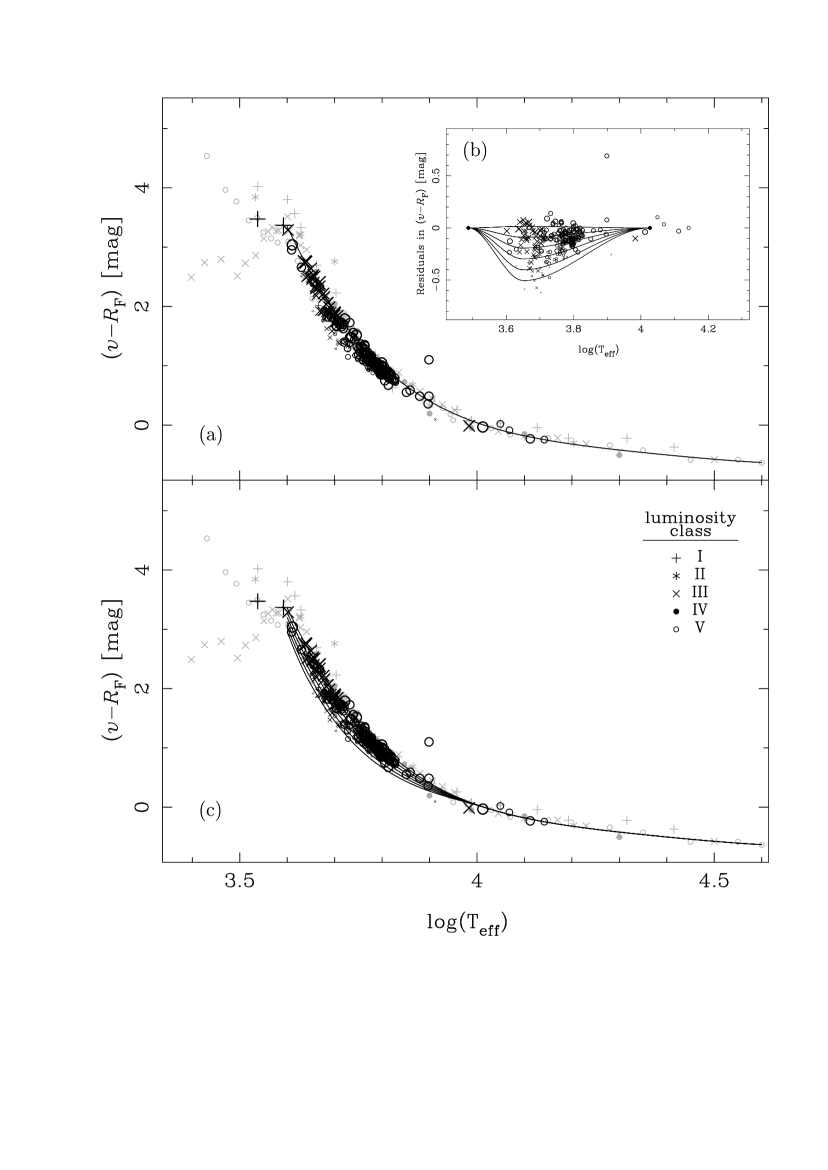
Figure 16: Variation of the $(v-R_{\rm F})$ colour as a function of effective temperature. Different symbols correspond to distint luminosity classes, as explained in the key, whereas symbol sizes are indicative of metallicity (larger symbols for higher [Fe/H]). In panel (a) and (c) we have overplotted, with light-grey symbols, the stellar sample of Pickles (1998). The inclusion of the latter has allowed us to obtain an initial fit only dependent on $T_{\rm eff}$ up to the highest temperature side. The inset in panel (b) corresponds to a zoom in the intermediate temperature interval (after subtracting the initial fit), where the dependence on metallicity is more important. A new set of polynomials where fitted in this interval to reproduce the behavior in both $T_{\rm eff}$ and [Fe/H] (where metallicities are [Fe/H]=$-2.0$, $-1.5$,$-1.0$, $-0.5$, 0.0, and $+0.5$ from bottom to top). The combination of these polinomyals and the initial fit leads to the final fitting functions displayed in panel (c). Note that these functions are not extrapolated below $\log(T_{\rm eff})<3.6$.

Figure 17: Comparison between the colour excess measured in the ($v-R_{\rm F}$) colour as a function of ficticious $E(B-V)$ artificially introduced in the spectra of the reddening free stellar subsample. Although we are using the same symbols than in Fig. 16, it is clear that the scatter introduced by distinct atmospheric stellar parameters is almost negligible. The relation is nicely fitted by a second order polynomial.

Figure 18: Comparison between $E(B-V)$ values from the literature with $E(B-V)$ estimations obtained from the excesses measured in the $(b4500-b6400)$ colour following the method described in this appendix.

References

- Alonso A., Arribas S., & Martinez–Roger (1996) Alonso A., Arribas S., Martínez–Roger C., 1996, A&A, 313, 873
- Beers et al. (1999) Beers T.C., Rossi S., Norris J.E., Ryan S.G., Shefler T., 1999, AJ, 117, 981
- Bohlin & Gilliland (2004) Bohlin R. C., Gilliland R. L., 2004, AJ, 127, 3508
- Bonifacio, Caffau, & Molaro (2000) Bonifacio P., Caffau E., Molaro P., 2000, A&AS, 145, 473
- Bruzual & Charlot (1993) Bruzual G., Charlot S., 1993, ApJ, 405, 538
- Bruzual & Charlot (2003) Bruzual G., Charlot S., 2003, MNRAS, 344, 1000
- Burstein et al. (1984) Burstein D., Faber S.M., Gaskell C.M., Krumm N., 1984, ApJ, 287, 586
- Burstein et al. (1986) Burstein D., Faber S.M., González J.J., 1986, AJ, 91, 1130
- Cappellari (2004) Cappellari M., Emsellem E., 2004, PASP, 116, 138
- Cardiel (1999) Cardiel N., 1999, Ph. D. Thesis, Universidad Complutense de Madrid
- Carney et al. (1994) Carney B.W., Latham D.W., Laird J.B., Aguilar L.A., 1994, AJ, 107, 2240
- Castro et al. (1997) Castro R.R., Rich R.M., Grenon M., Barbuy B., McCarthy J.K., 1997, AJ, 114, 376
- Cayrel de Strobel et al. (1997) Cayrel de Strobel G., Soubiran C., Friel E. D., Ralite N., Francois P., 1997, A&AS, 124, 299
- Cenarro et al. (2001) Cenarro A.J., Gorgas J., Cardiel N., Pedraz S., Peletier R.F., Vazdekis A., 2001b, MNRAS, 326, 981
- Chen et al. (1999) Chen B., Figueras F., Torra J., Jordi C., Luri X., Galadí–Enríquez D., 1999, A&A, 352, 459
- Dalle Ore et al. (1991) Dalle Ore C., Faber S.M., González J.J., Stoughton R., Burstein D., 1991, ApJ, 375, 427
- Dias et al. (2002) Dias W.S., Alessi B.S., Moitinho A., Lépine J.R.D., 2002, A&A, 389, 871
- Dyck et al. (1996) Dyck H.M., Benson J.A., van Belle G.T., Ridgway S.T., 1996, AJ, 111, 1705
- Faber et al. (1985) Faber S.M., Friel E.D., Burstein D., Gaskell C.M., 1985, ApJS, 57, 711
- Favata, Micela & Sciortino (1997) Favata F., Micela G., Sciortino S., 1997, A&A, 323, 809
- Feltzing & Gustafsson (1998) Feltzing S., Gustafsson B., 1998, A&AS, 129, 237
- Fernández-Villacañas (1990) Fernández–Villacañas J.L., Rego M., Cornide M., 1990, AJ, 99, 1961
- Fitzpatrick (1999) Fitzpatrick E.L., 1999, PASP, 111, 63
- Friedemann (1992) Friedemann C., 1992, Bull. Inf. Centre Donnes Stellaires, 40, 31
- González & Laws (2000) González G., Laws C., 2000, AJ, 119, 390
- Gorgas et al. (1993) Gorgas J., Faber S.M., Burstein D., González J.J., Courteau S., 1993, ApJS, 86, 153
- Gunn & Stryker (1983) Gunn J.E., Stryker L.L.,1983, ApJS, 52, 121
- Harris (1996) Harris W.E., 1996, AJ, 112, 1487
- Hauck & Mermilliod (1998) Hauck B., Mermilliod M., 1998, A&AS, 129, 431
- Jacoby (1984) Jacoby G.H., Hunter D.A., Christian C.A., 1984, ApJS, 56, 257
- Janes (1977) Janes K.A., 1977, PASP, 1977, 89, 576
- Johnson H.J., Morgan W.W. (1953) Johnson H.L., Morgan W.W., 1953, ApJ, 117, 313
- Jones (1997) Jones, L.A., 1997, Ph.D. Thesis, University of North Carolina, Chapel Hill
- Jones & Worthey (1995) Jones L.A., Worthey G., 1995, ApJ, 446, 31
- Kholopov (1998) Kholopov et al., 1998, Combined General Catalogue of Variable Stars
- King (1985) King, D., 1985, La Palma Technical Note 31
- Kirkpatrick et al. (1991) Kirkpatrick J.D., Henry T.J., McCarthy Jr D.W., 1991, ApJS, 77, 417
- Kollatschny (1980) Kollatschny W., 1980, A&A, 86, 308
- Kurtz (1984) Kurtz M.J., 1984, Garrison R.F., eds, Proc. of the Workshop in honour of W.W. Morgan and P.C. Keenan, University of Toronto, David Dunlap Observatory
- Le Borgne et al. (2003) Le Borgne J.-F., Bruzual G., Pelló R., Lancon A., Rocca-Volmerange B., Sanahuja B., Schaerer D., Soubiran C., Vílchez-Gómez R., 2003, A&A, 402, 433
- Le Borgne et al. (2004) Le Borgne J.-F., Rocca–Volmerange B., Prugniel P., Lançon A., Fioc M., Soubiran C., 2004, A&A, 425, 881
- Mallik (1998) Mallik S.V., 1998, A&A, 338, 623
- McWilliam (1990) McWilliam A., 1990, ApJS, 74, 1075
- Mermilliod et al. (1997) Mermilliod J.-C., Mermilliod M., Hauck B., 1997, A&AS, 124, 349
- Perrin (1998) Perrin G., Coude Du Foresto V., Ridgway S.T., Mariotti J.M., Traub W.A., Carlenton N.P., Lacasse M.G., 1998, A&A, 331, 619
- Pickles (1985) Pickles A.J., 1985, ApJS, 59, 33
- Pickles (1998) Pickles A.J., 1998, PASP, 110, 863
- Prugniel & Soubiran (2001) Prugniel P., Soubiran C., 2001, A&A, 369, 1048
- Prugniel & Soubiran (2004) Prugniel P., Soubiran C., 2004, preprint (astro-ph/0409214)
- Ramirez et al. (2000) Ramírez S.V., Sellgren K., Carr J.S., Balachandran S.C., Blum R., Terndrup D., Steed A., 2000, ApJ, 537, 205
- Randich et al. (1999) Randich S., Gratton R., Pallavicini R., Pasquini L., Carreta E., 1999, A&A, 348, 487
- Rose (1994) Rose J.A., 1994, AJ, 107, 206
- Sadakane et al. (1999) Sadakane K., Honda S., Kawanomoto S., Takeda Y., Takada–Hidai M., 1999, PASJ, 51, 505
- Savage et al. (1985) Savage B.D., Massa D., Meade M., & Wesselius P.R., 1985, ApJS, 59, 397
- Schiavon et al. (2002) Schiavon R.P., Faber S.M., Castilho B.V., Rose J.A., 2002, ApJ, 580, 850
- Schlegel, Finkbeiner, & Davis (1998) Schlegel D.J., Finkbeiner D.P., Davis M., 1998, ApJ, 500, 525
- Schuster et al. (1996) Schuster W.J., Nissen P.E., Parrao L., Beers T.C., Overgaard L.P., 1996, A&AS, 117, 317
- Serote Roos et al. (1996) Serote Roos M., Boisson C., Joly M., 1996, A&AS, 117, 93
- Silva & Cornell (1992) Silva D.R., Cornell M.E., 1992, ApJS, 81, 865
- Snow et al. (1994) Snow T.P., Lamers H.J.G.L.M., Lindholm D.M., Odell A.P., 1994, ApJS, 95, 163
- Spinrad (1962) Spinrad H., 1962, ApJ, 135, 715
- Spinrad & Taylor (1971) Spinrad H, Taylor B.J., 1971, ApJS, 22, 445
- Stetson, Bruntt & Grundahl (2003) Stetson P.B., Bruntt H., Grundahl F., 2003, PASP, 115, 413
- Stevenson (1994) Stevenson C.C, 1994, MNRAS, 267, 904
- Taylor (1999) Taylor B.J., 1999, A&AS, 134, 523
- Thomas et al. (2003) Thomas D., Maraston C., Bender R., 2003, MNRAS, 343, 279
- Thomas et al. (2004) Thomas D., Maraston C., Korn A., 2004, MNRAS, 351, 19
- Thorén & Feltzing (2000) Thorén P., Feltzing S., 2000, A&A, 363, 692
- Trager et al (1998) Trager S.C., Worthey G., Faber S.M., Burstein D., González J.J., 1998, ApJS, 116, 1
- Twarog et al. (1997) Twarog B.A., Ashman K.M., Anthony-Twarog B.J., 1997, AJ, 114, 2556
- Valdes et al. (2004) Valdes F., Gupta R., Rose J.A., Singh H.P., Bell D.J., 2004, ApJS, 152, 251
- Vazdekis (1999) Vazdekis A., 1999, ApJ, 513, 224
- Vazdekis & Arimoto (1999) Vazdekis A., Arimoto N., 1999, ApJ, 525, 144
- Vazdekis et al. (1996) Vazdekis A., Casuso E., Peletier F.R., Beckman J.E., 1996, ApJS, 106, 307
- Vazdekis et al. (2003) Vazdekis A., Cenarro A.J., Gorgas J., Cardiel N., Peletier R.F., 2003, MNRAS, 340, 1317
- Worthey (1994) Worthey G., 1994, ApJS, 95, 107
- Worthey & Ottaviani (1997) Worthey G., Ottaviani D. L., 1997, ApJS, 111, 377
- Worthey et al. (1994) Worthey G., Faber S.M., González J.J., Burstein D., 1994, ApJS, 94,68
- Zboril & Byrne (1998) Zboril M., Byrne P.B., 1998, MNRAS, 299, 753