The tails in the Helix Nebula NGC 7293

Abstract

Aims. We have examined a stream-source model for the production of the cometary tails observed in the Helix Nebula NGC 7293 in which a transonic or moderately supersonic stream of ionized gas overruns a source of ionized gas. We have compared the velocity structures calculated with the available observational data. We have also investigated the suggestion that faint striations visible in the nebular gas are the decaying tails of now destroyed cometary globules.

Methods. We have selected relevant results from extensive hydrodynamic calculations made with the COBRA code.

Results. The velocities calculated are in good agreement with the observational data on tail velocities and are consistent with observations of the nebular structure. The results also are indicative of a stellar atmosphere origin for the cometary globules. Tail remnants persist for timescales long enough for their identification with striations to be plausible.

1 Introduction

Many PNe contain extended cometary tail-like structures. These emanate from dense, neutral (Meaburn et al. 1992; Huggins et al. 1992) globules with radiatively ionized surfaces and point away, comet-like, from the central star. The most studied are those in the highly evolved PNe NGC 7293 (the Helix Nebula). A brief review of the two broad classes of models proposed to account for them is given by Dyson (2003). “Shadow” models (e.g., Van Blerkom & Arny 1972; Cantó et al. 1998; López-Martin et al. 2001) use an opaque cloud to shield gas from the direct radiation field of the PNe nuclear star. The shadow region is energized by a diffuse radiation field of different quality from the direct stellar field. “Stream-source” models (Dyson et al. (1993) - henceforth Paper I, Falle et al. (2002) - henceforth Paper II) are based on mass injection from embedded clumps in global flows. There are three relevant length scales (Hartquist & Dyson 1993). The smallest is the mass injection scale and the largest scale is that for assimilation of injected gas into the global flow. The intermediate scale where injected material largely retains its own identity, produces a tail feature that is dynamically affected by momentum transfer from the global flow.

Lefloch & Lazareff (1994) argued for tail formation during the photoionization of dense globules, a suggestion also made by Rijkhorst et al. (2006) who did not, however, present any models. Yet as shown by Pavlakis et al. (2001), the diffuse radiation field which was neglected by Lefloch & Lazareff (1994) can suppress tail formation if it has an intensity of a few percent of the direct stellar flux. Given that there are several thousand tails distributed throughout the nebula with concommitant variations in direct flux, diffuse flux and inevitably globule properties, it is hard to see how the tail system could be produced by this mechanism. Stream-source models also have the advantage that they are inherently dynamic in distinction to the majority of shadow models where the dynamics of the gas is neglected, though the model of López-Martin et al. (2001) includes a flow of ionized gas perpendicular to a tail feature as the gas exits from a D-critical ionization front at the ionized sound speed. However, the only detailed observational study of the velocity structure of the Helix tails by Meaburn et al. (1998) shows no evidence for significant ionized gas velocities perpendicular to the tails.

The ratio of tail length to head diameter of the Helix cometary features ranges from $\approx 1$ to $\approx 100$ in the spectacular knot 38 (Meaburn et al. 1998) which has a deprojected actual tail length of $\approx 2.5\times 10^{17}\;{\rm cm}$. Tails are aligned to within a few degrees along radial vectors originating at the central star. Our discussions are directed specifically at the Helix tails and clumps and their generalisation to other PNe may be inappropriate.

In this paper we re-examine the stream-source models proposed in Paper I using extensive calculations of stream-source interactions by Dyson et al. (in preparation - henceforth Paper IV). In Paper I, a hot subsonic stream of bottled-up shocked stellar wind gas was assumed to interact with a source of cooler gas to produce tails. Serious objections to this tail generation mechanism were raised by O’Dell (2000) and Meaburn et al. (2005). The main problem is that the central cavity in the Helix is occupied by a hot ($T_{\rm e}\mathrel{\hbox to0.0pt{\lower 3.0pt\hbox{$\sim$}\hss}\raise 2.0pt\hbox{$>$}}2\times 10^{4}\;{\rm K}$) He⁺ emitting gas and it is hard to see where the hot shocked stellar wind gas resides. In fact much earlier, Meaburn & White (1982) had raised a similar objection because of the presence of an inner [OIII] emitting shell that would shield the cometary globules from the direct impact of any fast (subsonic or supersonic) wind.

Therefore we examine the suggestion that the cometary tail heads are overrun by a transonic or supersonic stream of photoionized gas (Meaburn et al. 1992, 1998; O’Dell 2000; Meaburn et al. 2005). We compare results with the knot dynamics observed by Meaburn et al. (1998) and show these are reasonably well reproduced. We briefly discuss the significance of clump motions for these models.

Meaburn et al. (2005) noted the existence of “headless” radial spokes close to the central star of NGC 7293 and suggested that these spokes were tails left behind after their cometary knots were photoevaporated away. Henry et al. (1999) and O’Dell et al. (2004) also noted similar striations in the nebular gas. We examine the effects of switching off the mass injection and show that tails persist for typical timescales of thousands of years before they are advected away by the stream flow, lending plausibility to the suggested origin (Meaburn et al. 2005).

2 Stream-source tail production

Paper I argued that long thin tails are produced only when subsonic streams interact with subsonic mass injection (all Mach numbers are defined in the reference frame of the clump). Paper II dealt with the interactions of hypersonic and transonic streams with injected matter. Pittard et al. (2005, henceforth Paper III) investigated the interaction of hypersonic flows with multiple clumps and the interaction of transonic flows with two adjacent clumps. We will consider only single clump interactions although both photographs of tails and the recent estimate of 23000 cometary knots (Meixner et al. 2005) suggest multiple clump interactions might occur in the Helix.

In Papers I to III it was assumed that there was a large temperature contrast between a hot global flow and injected gas with the stream gas behaving adiabatically and the injected gas behaving isothermally. Tail dynamics and morphology are determined by the thermal behaviour and temperature contrast of the stream and source gas as well as by the Mach number of the incident stream. Paper IV investigates a broader range of incident Mach numbers and temperature contrasts using spherical clump geometry (Paper III shows that the differences between spherical and cylindrical geometry are small). Results are also given for the case where both stream and source gases behave isothermally. This is appropriate if the stream gas as well as the source gas is photoionized and we utilise these results here. Computational details are given in Papers III and IV.

An important result from these new calculations is that identifiable long thin tails persist to appreciably higher Mach number interactions than suggested in Papers I and II. This is quantified in Paper IV.

Mass loss from the clumps in the Helix is due to photoionization. Clump images show the mass injection is strongest in the direction towards the central star. In Paper III it was shown that anisotropic mass injection made very little difference to the flow morphology in the case of a hypersonic wind interacting with source material. Comparison of tail structures for subsonic and transonic stream interactions where there is anisotropic injection is given in Paper IV. Results for a mass injection rate contrast of 20:1 (front to rear) show small differences in the tail morphologies and tail velocity structures between the isotropic and anisotropic cases once the flow has gone a few injection radii. We use results for isotropic mass injection here.

Although the models of Paper IV are far more extensive than previously given, they have still a major simplification. They contain only two gas phases (stream and injected gas) which may mix. The Helix tails possibly represent a three phase system that includes ionised stream gas and both neutral and ionised injected gas (e.g., O’Dell & Handron 1996; O’Dell 2000). To treat this properly requires the inclusion of radiation transfer.

3 Tail production

Meaburn et al. (1998), O’Dell (2000) and Meaburn et al. (2005) have shown that it is likely that clumps are overrun by photoionized gas that may be ionized AGB wind possibly contaminated with evaporated knot gas. We consider tail formation in an interaction where photoionized gas overruns clumps that lose material by photoionization. An isothermal-isothermal assumption for the thermal behaviour of the stream and source gas is appropriate.

It is unlikely in general that the clumps are being overrun by the very hot He⁺⁺ gas since the clumps have an average outward velocity of $14\;\hbox{${\rm{\rm\thinspace km}{\rm\thinspace s}^{-1}\,}$}$ (Meaburn et al. 1998) and the hot gas is dynamically inert with an expansion velocity of less than $11\;\hbox{${\rm{\rm\thinspace km}{\rm\thinspace s}^{-1}\,}$}$ (Meaburn et al. 2005). On the other hand, there might be clumps that are overrun by this hot gas since the velocity dispersion of the knots is around $6-8\;\hbox{${\rm{\rm\thinspace km}{\rm\thinspace s}^{-1}\,}$}$ (Meaburn et al. 1998). The temperature contrast between the stream gas and injected gas may be high. O’Dell (1998) suggests that the temperature of the He⁺⁺ gas is in excess of $2\times 10^{4}\;{\rm K}$ (because of the lack of O⁺⁺ cooling). Henry et al. (1999) have modelled the ionization structure of the nebula and shown that the gas temperature drops from about $4\times 10^{4}\;{\rm K}$ near the star to $10^{4}\;{\rm K}$ at a distance where helium is about 50% in the form of He⁺⁺.

Meaburn et al. (1998) and Meaburn et al. (2005) favour the overrunning of clumps by expanding photoionized gas in the region where [OIII] is emitted. This gas has a temperature of about $10^{4}\;{\rm K}$ (Henry et al. 1999), and is overrunning the clumps with a velocity of about $17\;\hbox{${\rm{\rm\thinspace km}{\rm\thinspace s}^{-1}\,}$}$ relative to the clump global expansion velocity of $14\;\hbox{${\rm{\rm\thinspace km}{\rm\thinspace s}^{-1}\,}$}$.

The temperature of gas injected from the source is uncertain. O’Dell et al. (2005) note that the temperature of photoionized gas flowing from a clump towards the star decreases outwards from the density peak just behind the ionisation front on the clump surface. Some injection will occur from the sides of clumps where the diffuse radiation field softens the average photon energy leading to gas temperatures that could be a factor of around 2 lower than the temperature of gas excited by the direct radiation field (Van Blerkom & Arny 1972; Cantó et al. 1998).

As a reasonable range for the temperatures we use calculations from Paper IV for ratios of isothermal sound speeds ($c_{\rm S}/c_{\rm i}$, stream gas to injected gas) of 1:1 (equal temperatures) and 2:1 (a temperature ratio of 4:1). In Fig. 1 we give tail density structures for a sound speed ratio of 2:1 for incident stream Mach numbers $M=1,2,4$.

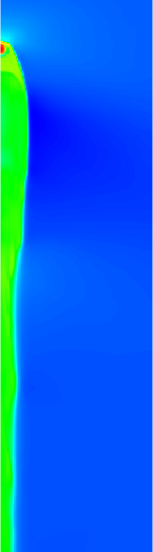
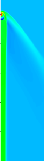
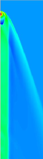
Figure 1: Tail density structures for sound speed ratio $c_{\rm S}/c_{\rm i}=$2:1. The stream Mach number, $M=1,2,4$ for the left, middle, and right panels respectively. Each panel shows a region $0<r<30$, $-100<z<10$. The logarithm of mass density is shown, with a scale of $-0.69$ to 0.39 (left), $-0.97$ to 0.99 (middle), and $-0.99$ to 1.60 (right). Blue denotes the lowest density, while red denotes the highest. The stream density is $0.25$. An injection region of unit radius is at the origin. See Paper II for further details about the computations.

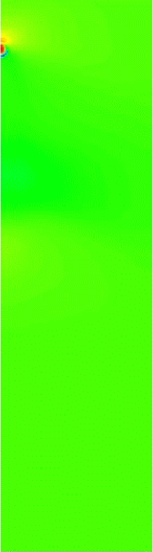
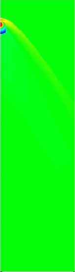
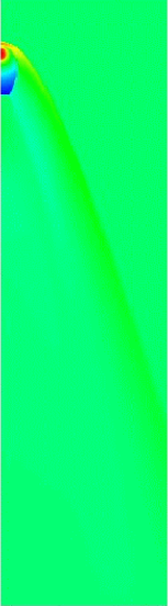
Figure 2: As Fig. 1 but for equal sound speeds with $M=1,2,4$ (left, middle, and right, respectively). The density scale extends from $-0.52$ to 0.39 (left), $-0.97$ to 0.99 (middle), and $-1.02$ to 1.59 (right). The stream density is 1.0.

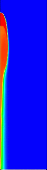
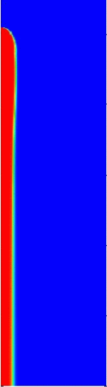
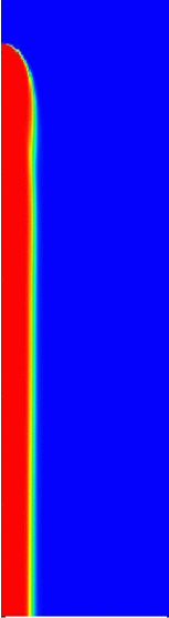
Figure 3: As Fig. 2 but showing advected scalar structures. Blue represents the stream gas, while red represents injected material (i.e. material evaporated from the clump into the flow).

In Fig. 2 we give the same information for a sound speed ratio 1:1. However a sound speed ratio of unity gives a tail density effectively the same as that of the stream and the plots of Fig. 2 therefore do not show systematic tail structure. The results of Paper IV demonstrate that the injected gas maintains its identity and there is very little mixing between it and stream gas. So to show this, we plot in Fig. 3 the advected scalar that distinguishes between the stream and injected gases. A recognisable tail of injected gas is embedded in stream gas. Some difference in emission or absorption properties (e.g., a different gas-to-dust ratio) is needed to make the tail visible as is clear from the density plot but it is a dynamical possibility for tail production.

4 Tail velocity structures

Important diagnostic information comes from the tail velocity structure in knot 38 given by Meaburn et al. (1998). In view of our model limitations, we use mass-weighted velocities for comparison with the data.

In Fig. 4 we show mass-weighted velocity profiles along tails for several incident Mach numbers and two stream-source gas temperature ratios. We give results only for the transonic and supersonic isothermal-isothermal flows that are relevant to the present paper.

Figure 4: $V_{\rm Z}$ vs $z$ for $M=1,2,4$, and sound speed ratios 1 and 2 (i.e. temperature ratios 1 and 4). The injection radius is $r_{\rm c}$.

For streams that are roughly in excess of transonic, the velocity increases quickly over a few injection radii. The initial increase is followed by a velocity decrease for Mach numbers less than about 3 then the velocity rises to a roughly coasting velocity. Once the Mach number is around 3, the initial increase is just followed by a very gentle rise or even roughly constant velocity over distances of tens of injection radii. Appreciably greater distances are probably not relevant to the Helix tails where the very longest tail (knot 38) has a length about 100 times its head diameter and we display results accordingly.

The final velocity reached depends on the temperature contrast between the stream and source gas and is higher (in terms of the stream velocity, $V_{\rm S}$) the lower the temperature contrast. This is as expected since the temperature contrast determines crudely the stream-injected gas density contrast and there is more momentum transfer from unit mass of the stream to unit mass of injected gas the less this contrast. At sufficiently high incident Mach number and low enough temperature contrast, the tail material achieves supersonic velocities in terms of the sound speed in the stream and obviously as well that of the injected gas (since the injected gas is either at the same temperature or cooler than the stream gas).

To compare the tail models with the observational data we assume that a stream of velocity $V_{\rm S}$ interacts with a clump which has a velocity $V_{\rm C}$, where both velocities are measured in the stellar frame. The relative velocity is therefore ($V_{\rm S}-V_{\rm C}$). We concentrate on knot 38 of Meaburn et al. (1998). The gas at the end of this tail has a velocity $V_{\rm T}=22\;\hbox{${\rm{\rm\thinspace km}{\rm\thinspace s}^{-1}\,}$}$ relative to the head (Meaburn & Redman 2003). Since this knot has a tail length-to-head diameter ratio of around 100:1 we take this to be equal to the coasting velocity from our calculations reached at 100 injection radii.

We can write $V_{\rm T}=\beta(M)(V_{\rm S}-V_{\rm C})=\beta(M)Mc_{\rm S}$ where $\beta(M)$ is a constant dependent on the Mach number $M$ of the interaction and the stream-source sound speed ratio and $M\equiv(V_{\rm S}-V_{\rm C})/c_{\rm S}$. In Table 1 we give values of $\beta(M)$ for the cases considered here.

Table 1: The value of $\beta(M)$ as a function of $M$ and $c_{\rm S}/c_{\rm i}$.

M	$c_{\rm S}/c_{\rm i}=1$	$c_{\rm S}/c_{\rm i}=2$
1	0.91	0.76
2	0.81	0.54
4	0.66	0.43

In Table 2 we give tail velocities calculated for various Mach numbers for the two temperature ratios above using the global knot velocity of $14\;\hbox{${\rm{\rm\thinspace km}{\rm\thinspace s}^{-1}\,}$}$. We use a sound speed of $11.7\;\hbox{${\rm{\rm\thinspace km}{\rm\thinspace s}^{-1}\,}$}$ (i.e. $c_{\rm i}=10^{4}\;{\rm K}$) for the source gas. We also list values of $V_{\rm S}$, the stream velocity in the stellar frame, for comparison with the value of $31\;\hbox{${\rm{\rm\thinspace km}{\rm\thinspace s}^{-1}\,}$}$ of the overrunning stream found by Meaburn et al. (1998).

The observed acceleration towards positive radial velocities along the tail from knot 38 is shown particularly well in the line profiles in Fig. 13 of Meaburn et al. (1998) and in the velocity images in Figs. 4 and 12 of that paper (though first correct the error in the legend for Fig. 12 which includes four panels whose indicated positions should all be reversed i.e. bottom-left, bottom-right, top-left, top-right should read top-right, top-left, bottom-right, bottom-left respectively). With this correction it can be seen in Fig. 12 that the tail furthest from the knot becomes more prominent in the more positive radial velocity range.

Table 2: Tail ($V_{\rm T}$) and stream ($V_{\rm S}$) velocities (${\rm{\rm\thinspace km}{\rm\thinspace s}^{-1}\,}$).

	$c_{\rm S}/c_{\rm i}=1$		$c_{\rm S}/c_{\rm i}=2$
M	$V_{\rm T}$	$V_{\rm S}$	$V_{\rm T}$	$V_{\rm S}$
1	11	26	18	38
2	19	37	25	61
4	31	61	40	107

We see that the tail and overrunning stream velocities are reasonably well reproduced with $M\approx 2$, $c_{\rm S}/c_{\rm i}=1$ and $M\approx 1$, $c_{\rm S}/c_{\rm i}=2$.

Tails should show more complex velocity structure closer to the injection zone particularly with anisotropic mass injection but we do not consider this further here.

The setting up time for the tail of knot 38 $\approx 2-4\times 10^{3}\;{\rm yrs}$ with a length of $2.5\times 10^{17}\;{\rm\thinspace cm}$ and a tail gas velocity of $10-20\;\hbox{${\rm{\rm\thinspace km}{\rm\thinspace s}^{-1}\,}$}$. This implies formation after fast wind activity has ceased. Although Patriarchi & Perinotto (1991) showed from IUE observations that 60% of central stars of PNe emit fast particle winds, Cerruti-Sola & Perinotto (1985) failed to detect one from the central star of NGC 7293. Shorter tails take proportionally shorter times to form and more “typical” tails with lengths of a few times $10^{15}\;{\rm\thinspace cm}$ could be set up in timescales of the order of a hundred years. It is not clear why the tails are generally fairly short. One possibility might be time fluctuations in stream or source injection properties.

5 Clump motions

The effects on tail production mechanisms of systematic clump motions, radial or non-radial, have received little attention. The non-radial component of the Helix knot expansion velocity is unclear. On general grounds, non-radial velocity components of clumps seem inevitable if clumps form in dynamical instabilities. If they are generated by shell fragmentation, they should have some dispersion around the shell velocity at fragmentation since it is highly unlikely that shells are strictly spherical.

Diamond & Kemball (2003) measured global proper motions of the SiO maser spots in the Mira variable TX Cam that correspond to velocities of about $10\;\hbox{${\rm{\rm\thinspace km}{\rm\thinspace s}^{-1}\,}$}$ and noted that “significant” non-radial velocity components are present. These motions are in a stellar atmosphere of radius $\sim{\rm few}\times 10^{13}\;{\rm\thinspace cm}$. If these spots move out to radial distances $\sim 10^{17}\;{\rm\thinspace cm}$, conservation of angular momentum ensures very small non-radial velocity components ($\ll 1\;\hbox{${\rm{\rm\thinspace km}{\rm\thinspace s}^{-1}\,}$}$).

In Paper IV results are given for situations where clumps move at an angle to a global flow. To a good approximation, well-developed tails lie along the resultant velocity vector of the stream-clump velocities. If we assume that the stream is strictly radial, then tails are aligned to an angle $\alpha\approx{\rm arc\;\;tan}[V_{\rm tan}/(V_{\rm S}-V_{\rm C})]$ with the radial direction, where $V_{\rm tan}$ is the non-radial velocity component of the clump velocity. In Table 3 we give maximum values of $V_{\rm tan}$ that allow an alignment angle of 5^∘ to the radial direction where we take this angle as characteristic.

Table 3: $V_{\rm tan}$ (${\rm{\rm\thinspace km}{\rm\thinspace s}^{-1}\,}$) for an alignment angle of 5^∘.

M	$c_{\rm S}/c_{\rm i}=1$	$c_{\rm S}/c_{\rm i}=2$
1	1	2
2	2	4
3	4	8

The best-fit cases for $V_{\rm T}$ and $V_{\rm S}$ detailed above require very small values of $V_{\rm tan}$ ($\mathrel{\hbox to0.0pt{\lower 3.0pt\hbox{$\sim$}\hss}\raise 2.0pt\hbox{$<$}}2\;\hbox{${\rm{\rm\thinspace km}{\rm\thinspace s}^{-1}\,}$}$) for alignment. This is unlikely to be satisfied with shell instability formation but is more consistent with the much lower non-radial velocity components expected if the clumps originated in stellar atmospheres.

6 Tail persistence

We have examined the persistence of tails where the injection is switched off to quantify the proposal by Meaburn et al. (2005) that this is responsible for the production of headless spokes. In Fig. 5 we show time frames for the evolution of the tails produced for the two best fit cases in Section 4 (i.e. $M\approx 2$, $c_{\rm S}/c_{\rm i}=1$ and $M\approx 1$, $c_{\rm S}/c_{\rm i}=2$). As before, for the case of a sound speed ratio of unity we give both the advected scalar plots and the density plots. Tails persist over timescales of at least 50 or so (in dimensionless units). The actual time unit is equal to $2r_{\rm C}/V_{\rm F}$, where $V_{\rm F}$ is the gas velocity in the clump frame (i.e. $V_{\rm S}-V_{\rm C}$). If we take the sound speed in the injected gas to be $11.7\;\hbox{${\rm{\rm\thinspace km}{\rm\thinspace s}^{-1}\,}$}$ as before, the flow speed in both cases is $23.4\;\hbox{${\rm{\rm\thinspace km}{\rm\thinspace s}^{-1}\,}$}$. If we take the injection radius as about $10^{15}\;{\rm\thinspace cm}$ corresponding to a typical clump diameter, the tails persist for times at least $\sim 1400\;{\rm yr}$. It appears plausible therefore that headless tails are the remains of tails behind recently destroyed clumps.

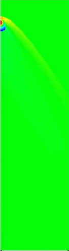
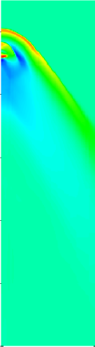
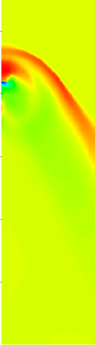
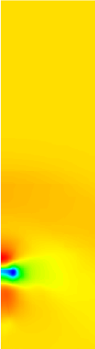
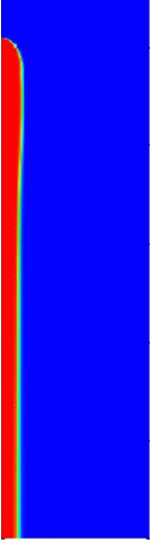
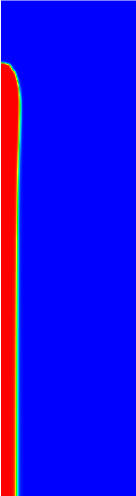
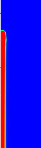
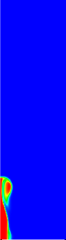
Figure 5: Evolution of the $M=2$, $c_{i}/c_{s}=1.0$ isothermal-isothermal simulation after the source injection is switched off. t=0 (left), 6.0, 13.4, 28.3, and 58.0 (right). The isothermal sound speed=1.0 for both the injected and ambient flow, and the ambient flow speed=2.0. The top panels show density plots, while the bottom panels show the tracer for injected material. The colour scaling of each density panel is different in order to best display the structure. From left to right, ${\rm log_{10}}\;\rho=-0.97$ to 0.99, $-0.14$ to 0.28, $-0.38$ to 0.15, $-0.38$ to 0.12, and $-0.28$ to 0.08. The density enhancement relative to the stream density (${\rm log_{10}}\;\rho=0.0$) declines as time evolves.

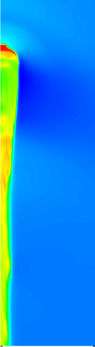
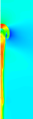
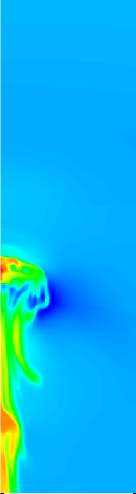
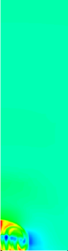
Figure 6: Evolution of the $M=1$, $c_{\rm S}/c_{\rm i}=2$ isothermal-isothermal simulation after the source injection is switched off. $t=0$ (left), 10.9, 21.7, 43.4, 76.4, and 120.4 (right). The isothermal sound speed=1.0 and 2.0 for the injected and ambient flow (respectively), and the ambient flow speed=2.0. The colour scaling of each panel is different in order to best display the structure. From left to right, ${\rm log_{10}}\;\rho=-0.69$ to 0.39, $-0.70$ to 0.11, $-0.81$ to 0.04, $-0.81$ to 0.03, $-0.74$ to 0.04, and $-0.74$ to $-0.32$. The density enhancement relative to the stream density (${\rm log_{10}}\;\rho=-0.60$) declines as time evolves.

7 Conclusions

Linear structures have been observed in several planetary nebulae. This morphology has led to two classes of models. However morphology itself is not sufficient to discriminate between them. Velocity structure is the key and only for two knots (14 and 38) in the Helix nebula is the necessary data available. The acceleration along the tail associated with the spectacular knot 38 suggests strongly that there is momentum transfer between a directed flow and a mass source. The advanced evolutionary state of the central star, and the details of the nebular structure, rule out any hypersonic stellar wind-mass source interaction. Although attractive in many respects, the interaction with a subsonic hot stream of shocked stellar wind gas is also ruled out because the existence of a reservoir of hot gas cannot be reconciled with the nebular structure. Much more plausible is tail formation taking place when a transonic or moderately supersonic stream of photoionized gas overruns gas injected by the photoionization of cometary globules. The injected gas is accelerated by momentum transfer from the stream and the velocities that are generated are in good agreement between those measured for the likely overrunning stream and the tail gas of knot 38 in the Helix. Thus the general scheme for the formation of cometary globules involves flows (or winds) overrunning a slowly expanding system of pre-existing dense neutral globules. At least for NGC 7293, the knotty nature of the ambient neutral shells associated with this object surely precludes any other possibility (instabilities in a global expanding shell for example). In fact the very strong radial alignment of the tails suggests that when overrun, the globules have a velocity that can at most have a very small non-radial component. This is consistent with density structures that originate at radii far less that the present scale size of the nebula. Finally, it also appears likely that the widely distributed striations seen in the nebular gas represent the remains of tail structures generated by mass injection from now destroyed globules.