Lensing signals in the Hubble Ultra-Deep Field
using all 2nd order shape deformations

Abstract

The long exposure times of the HST Ultra-Deep Field plus the use of an empirically derived position-dependent PSF, have enabled us to measure a cardioid/displacement distortion map coefficient as well as improving upon the sextupole map coefficient. We confirmed that curved background galaxies are clumped on the same angular scale as found in the HST Deep Field North. The new cardioid/displacement map coefficient is strongly correlated to a product of the sextupole and quadrupole coefficients. One would expect to see such a correlation from fits to background galaxies with quadrupole and sextupole moments. Events that depart from this correlation are expected to arise from map coefficient changes due to lensing, and several galaxy subsets selected using this criteria are indeed clumped.

1 Introduction

This letter expands upon previous work of two of us (Irwin and Shmakova, 2003b, 2005), hereafter [IS], aimed at identifying lensing signals created by small-scale structure and substructure, the ultimate purpose being the development of a unique small-scale cosmological signal.

In [IS] we described and developed a non-linear lensing method based on a complex power series lensing distortion map. The map is derived from a symplectic coordinate transformation from a reference frame at the telescope to a reference frame at the source galaxy. It has a succinct complex power series form: $w_{S}=w+a\bar{w}+b\bar{w}^{2}+d_{1}w\bar{w}+d_{2}w^{2}$, where $w=x+iy$ represents the position relative to the beam centroid. This map is a generalization of the usual linear weak lensing relationship. Each term in the series is a rotational eigenvector and creates a distinct distortion of an azimuthally symmetric source galaxy. There are two well-known linear terms: an amplification (“convergence”) and a term that produces a quadrupolar distortion (“shear”). For lensing $a(=a_{L})=-\gamma$.

The three 2nd-order map terms are: a sextupolar triangle-like distortion, a cardioid distortion, and a quadratically increasing displacement of circles. Since lensing simultaneously produces both the cardioid ($d_{2}$) and displacement ($d_{1}$) terms, they can be denoted by a single coefficient ($d$), with $d_{1}=2d$ and $d_{2}=\bar{d}$ . We call the so-combined $d$-terms the “cardioid/displacement” term. See fig.1 for examples of these shape distortions.

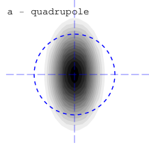
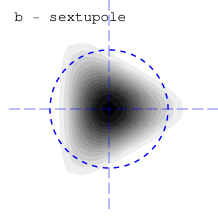
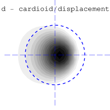
Figure 1: Shape deformations coming from different terms of a map. The dashed circles correspond to an original isophote. These pictures demonstrate the deformation due to the presence of single terms: either $a_{x}=0.3,\,b_{x}=-0.06,\,d_{x}=0.02$.

The lensing distortion map embodies a distinction between intrinsic galaxy shapes and allowed lensing distortions of that shape. The power of this approach will become particularly evident here as we expand our consideration to include all 2nd-order map coefficients. The interrelationship of these coefficients allows one to infer whether a particular background galaxy is likely to have been lensed.

In [IS] the lensing distortion map formalism was applied to the Hubble Deep Field North (HDFN). PSFs generated by TinyTim were convolved with mapped radial profiles. Parameters for the map and the radial profile were simultaneously determined by a least-squares fit to the background galaxy intensity matrices. Curved background galaxies, defined by the relative orientation (for that galaxy) of the quadrupole and sextupole map coefficients, were found to be spatially clumped when compared to randomly selected background galaxy subsets, suggesting that some fraction of curved galaxies are the result of lensing by foreground haloes and/or subhaloes. We find it improbable that the observed clumping could arise from intrinsic alignment of background galaxies since the members of identified clumps have a wide range of z-values.

We report here the results of extending that analysis to the HST Ultra-Deep Field (UDF). Due to the longer UDF exposure and access to an empirically derived time-averaged field-dependent PSF for the Hubble wide-field camera (WFC)(Anderson and King, 2006), we have again observed the clumping of curved galaxies and we have successfully measured an additional second-order map coefficient representing the cardioid/displacement distortion.

We find a strong correlation between the the cardioid/displacement coefficient and a product of the quadrupole and sextupole map coefficients. Such a correlation is expected from a fit to background galaxy shapes. Galaxies that do not comply with this correlation may be considered as candidates for quadrupole or sextupole lensing or both. We present results supporting this hypothesis.

2 UDF data processing

The F606W UDF data set which we analyze in this paper consists of 112 half-orbit exposures. Each exposure was taken at a different pointing, with two primary orientations that were rotated by $\approx 90^{\circ}$. We transformed each frame of the field into a distortion-free frame which one of us (Anderson, 2005) had constructed for the WFC.

Using the distortion-free transform of the first UDF frame as a frame of reference and bright point-like galaxies as locaters, we next determined linear transformations between the distortion-free transform of each of the remaining frames and this reference frame. These transformations were then used to map the center of each pixel in each frame into the reference frame. We removed the sky from the images by examining pixels in 800x800 patches and setting the background to zero.

The construction of the super-image is an iterative process. The super-image is chosen to be 2x super-sampled with respect to the image pixels. To construct this 8200x8200 super-image, we proceed pixel-by-pixel finding the closest corresponding pixel in each individual frame. This provides 112 independent estimates of the flux for each pixel. Since the individual frames have slightly different exposure times, we divide the flux by the ratio of the image’s exposure to a reference-image exposure time of 1200 seconds. We employ simple sigma-clipped averaging to find a representative value for that pixel, obtaining a first super-image estimate. Only one out of four pixels is statistically independent.

So that the super image can be interpolated without high frequency noise we smooth the first composite image with the kernel

$$\left[\matrix{0.0625&0.1250&0.0625\cr 0.1250&0.2500&0.1250\cr 0.0625&0.1250&0.0625}\right].$$

Then for each pixel in each individual exposure, we find the difference between it and the interpolated super-image (from the first iteration), thereby obtaining 112 frames of residuals. We add the sigma-clipped average of these residuals to the original pixel value, to get the final value of each super-image pixel.

To ensure that the galaxy shapes we are measuring are intrinsic to the galaxies and not artifacts of the detector, we propagate the model PSFs through the same stacking procedure as used for the galaxy images. To get a PSF appropriate for our super images, we generated an array of artificial stars in our reference frame. The stars had total fluxes of $10^{5}$ photons and were separated by $\sim 100$ pixels and placed with pixel phases of $(0,0)$, $(0.5,0)$, $(0,0.5)$ and $(0.5,0.5)$. We used the inverse transformations to determine where each of these stars landed in each of the 112 exposures, and then used the spatially variable PSF model of Anderson and King (2006) to generate an artificial set of exposures with this grid of stars in them.

Finally, we combine together the PSFs at different pixel phases to get a x4 representation of the PSF. It is this x4 PSF which we convolve with a x4 mapped radial profile to find the best fit to each galaxy image.

Since the fit procedure to find map parameters is designed to analyze galaxies with a single dominant peak, we have developed software to identify and select such galaxies. This software identifies all peaks within each galaxy (previously selected using SExtractor softwareBertin and Arnouts (1996)) and based on criteria such as separation, flux, and pixel height, decides whether these peaks should be considered part of a single peak. After all peaks are processed then, based upon a second set of criteria such as total flux and maximum-to-minimum height ratio, satisfactory central-peak regions are chosen to represent selected galaxies.

The fit-method is the same as that described in Section 3.3 of [IS]. The radial profile is taken to be a quadratic polynomial in $r^{2}$ times a Gaussian. A condition is imposed that the polynomial be positive. The map has four pairs of parameters: the centroid, the real and imaginary quadrupole coefficients, the real and imaginary sextupole coefficients, and the real and imaginary cardioid/displacement coefficients. The procedure begins by determination of the full-width-half-maximum of the image and its ellipticity. Then, without yet introducing the PSF, the radial profile and map coefficients are fit using a least-square difference with the selected region of the galaxy intensity matrix. Convolutions with ever larger footprint PSFs are similarly fit until the final PSF is convolved with the mapped radial profile and fit.

The distributions of the magnitudes for the quadrupole, sextupole, and cardioid/displacement coefficients of background galaxies $(z>0.5)$ are shown in fig. 2. The radial spreading caused by the PSF causes the map coefficients to be smaller then they are for the pre-PSF shape.

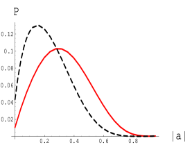
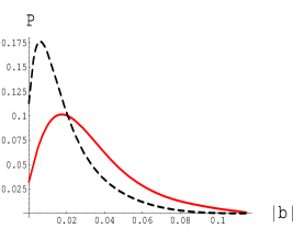
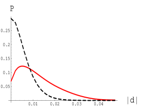
Figure 2: Distributions of the magnitude of the quadrupole coefficients ($a$, left panel), the sextupole coefficients ($b$, center panel), and the cardioid/displacement coefficients ($d$, right panel), of background galaxies using the radial-fit method without PSF (dashed) or the model method with the PSF (solid).

3 Clumping of curved galaxies

We looked for evidence of a spatial clumping of both curved and aligned galaxies as found in our HDFN analysis. The UDF was observed with the WFC camera which has a 2x smaller pixel size than the WFPC used for the HDFN. Because the total exposure time is about 10x longer, we were able to resolve 3 times more background galaxies per sq. min. We have used a different image stacking process and a different, empircally based PSF determination method. Strikingly, we find clumping of curved galaxies in the UDF at the same spatial angular scale as found in the HDFN. If lensing is the source of the clumping, it follows that the scattering lenses are similar in size and mass distribution. The probability of the observed clumping being random in the UDF is found to be $\approx 1\%$, as compared to our result of $4\%$ in the HDF. The distribution of the number of neighbors in circles of radius R=500 pixels is shown in fig.3. $1\%$ is the probability that randomly chosen subsets (of all background galaxies) with the same number of galaxies as the curved set have as many galaxies with N=8 or more neighbors as the curved set.

The clumping we observed for aligned galaxies in the HDFN is very weak in the UDF.

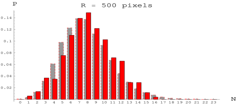
Figure 3: The foreground bars show the distribution of the number of curved neighbors in circles of radius R=500 pixels for the set of all curved galaxies. The background shows the same distribution averaged over randomly chosen subsets of galaxies with the same number of members. 500 pixels corresponds to 12 arcsec. Note the consistent shift to higher numbers of neighbors.

4 Correlations in background galaxy shapes

For our UDF images we have been able to measure the magnitude and orientation of an additional 2nd-order lensing-distortion-map coefficient, which we have referred to as the cardioid/displacement coefficient, or $d$-term. The $d$-term distorts the variable $r_{S}^{2}=w_{S}\bar{w}_{S}$ in the argument of an azimuthally-symmetric light stream profile with an amplitude proportional to $r^{3}\cos(\theta-\theta_{d})$. To our knowledge this is the first measurement of this coefficient with sufficient precision to exhibit the fundamental correlation we now describe.

We find the orientation of the $d$-term coefficient ($\theta_{d}$) to be correlated with the $\bar{a}b$ orientation ($\theta_{b}-\theta_{a}$). Scatter plots of $\theta_{d}$ vs. ($\theta_{b}-\theta_{a}$) are shown in the left and center panels of fig. 4. The center plot, in which the correlation is obvious, includes the PSF during the fit whereas the left plot, which barely has an indication of the correlation, ignores the PSF, illustrating the significance of the accuracy of the PSF treatment. We have studied the properties of the PSFs and find no evidence there for this correlation.

A projected distribution of galaxy count vs. $\theta_{d}-(\theta_{b}-\theta_{a})$ is shown for all galaxies in the left panel of fig. 5, and for curved galaxies in the center panel. For comparison, in the right panel we show the shape that would be predicted for an underlying delta-function correlation that incorporates the noise as predicted from a Fisher matrix study of the determination of these angles. The widths are similar, suggesting that the underlying correlation, though not necessarily a delta function, is indeed considerably sharper.

As the reference frame of the galaxy is rotated, the angles $\theta_{d}$ and $\theta_{b}-\theta_{a}$ increase linearly, explaining why the correlation in the center panel of fig.4 lies along a line of unit slope, and making it evident that this correlation is invariant under rotation. A feature of the PSF or an effect such as CTE (charge transfer efficiency), would not possess rotational invariance, and thus could not lead to such a correlation.

Another perspective on this correlation can be seen by plotting the real (imaginary) part of $d$ versus the real (imaginary) part of $\bar{a}b$. This is done in the right panel of fig. 4. One sees a general tilt to this diagram along the line $d=\frac{3}{5}\bar{a}b$. The factor $3/5$ has been determined, to a few percent, by a least-squares fit of a line to the data.

As a guide to find further correlations, one can use the moment methods of section 3.2 in [IS] to find the relationship $d-\frac{4}{5}a\bar{d}=\frac{1}{5}\bar{a}b-\frac{1}{5}(1-|a|^{2})m_{21}$ where $m_{21}\equiv\frac{M_{21}}{M_{22}}$ and $M_{nm}=\int w^{n}\bar{w}^{m}idA$. This equation was derived assuming an azimuthally symmetric root galaxy was mapped to fit a background shape. $M_{21}$ and $M_{22}$ are moments of the image of the root galaxy after the mapping.

An equation of this form is to be expected from general considerations. The quantities $d$, $b$, and $m_{21}$ are small enough that they occur only in first order. Furthermore as the reference coordinate system is rotated, $d$, $\bar{a}b$, $m_{21}$, $a^{2}\bar{b}$, $a\bar{d}$, and $a\bar{m}_{21}$ all rotate as vectors, so only these quantities can be involved. The terms with $m_{21}$ and $a\bar{m}_{21}$ can be added together and treated as the unknown. And only one of the two quantities $a\bar{d}$ and $a^{2}\bar{b}$ need be retained, as they are redundant.

Minimizing the (combined) $m_{21}$ term results in the approximate equation

$$d-\frac{4}{5}a\bar{d}\approx\frac{3}{5}\bar{a}b-\frac{1}{5}(1-|a|^{2})m_{21}.$$ (1)

The $3/5\,\bar{a}b$ and $4/5\,a\bar{d}$ are good fits to the data, and an additional $a^{2}\bar{b}$ term, if present, has a very small coefficient. The $1-|a|^{2}$ dependence of the coefficient of $m_{21}$ was adopted from the moment equation.

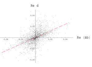
Figure 4: The angle of the d-term ($\theta_{d}$) vs. the angle of $\bar{a}b$ ($\theta_{b}-\theta_{a}$), without including the PSF (left panel) and including the PSF (center panel). The right plot shows $Re[d]$ vs. $Re[\bar{a}b]$.

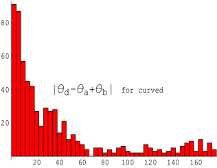
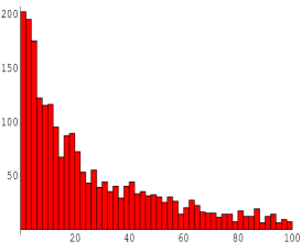
Figure 5: The left (center) panel shows the distribution of the angular difference $|\theta_{d}-(\theta_{b}-\theta_{a})|$ mod $180^{\circ}$ for all (curved) galaxies. The right panel shows our estimate, based on Fisher matrix calculations for each galaxy, of the expected measurement spread in $|\theta_{d}-(\theta_{b}-\theta_{a})|$ for a $\delta$-function correlation.

5 Evidence for cardioid/displacement lensing

The utility of the lensing-distortion-map parameterization is that if a background galaxy is subsequently lensed, this correlation, expressed in terms of the observed total $a\approx a_{L}+a_{S}$ and $b\approx b_{L}+b_{S}$, where $L$ indicates lensing and $S$ denotes the fit to the background source galaxy, would break down even if the lensing is quadrupole lensing alone. In other words, we know that in the presence of lensing, the map coefficients representing the shape of the source galaxy will add linearly to the lensing map coefficients. Since a contribution from lensing can be expected to change these coefficients, lensing will disturb this correlation condition. This will show up as a larger magnitude of $m_{21}$ when it is calculated using eq.1, because the change in $3/5\,\bar{a}b$ will be vectorially added to the existing $m_{21}$.

Hence if we choose those galaxies that are in the tail of the $|m_{21}|$ distribution (see the left panel of fig.6) they should be more likely to be lensed galaxies. We chose the cut at $|m_{21}|>0.023$ to end up with $\approx 200$ galaxies. Sets with less than 200 members have poorer statistics for clumping studies. The neighbor distribution for galaxies with $|m_{21}|>0.023$ is shown in the central panel of fig.6. It has a very small probability of occurring randomly, less than $1\%$.

Additionally we have investigated the small but tantalizingly distinct hump in the distribution of the curved galaxies shown in fig. 5 near $\theta_{d}-(\theta_{b}-\theta_{a})=180^{\circ}$. For these galaxies the sign of the coefficient of $d$ is opposite to that of $\bar{a}b$. This is the orientation for lensing events that are non-zero for all three lensing coefficients, and for which the $d$-term coefficient would be responding to the presence of $\Sigma^{\prime}$ (the gradient of the projected mass density function) in the lensing plane.

Since this is a small set of galaxies, it is difficult to convincingly establish lensing as a probable cause of this hump by a study of clumping probabilities. However we have done that, and when compared to randomly chosen curved galaxies of the same size, it has a probability of arising randomly of $\approx 3\%$. It is perhaps more convincing to look directly at the neighbors distribution, as shown in the right panel of fig.6. The neighbors distribution is compared for three distinct subsets of curved galaxies having the same number of members. The galaxy subset with $150^{\circ}<\theta_{d}-(\theta_{b}-\theta_{a})<180^{\circ}$ clearly has larger numbers of neighbors. Though this is suggestive, we would not claim to have conclusively observed $\Sigma^{\prime}$ lensing.

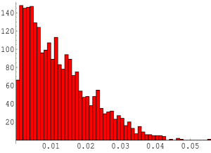
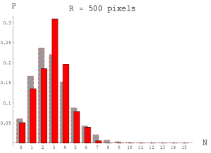
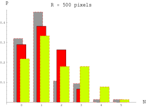
Figure 6: The left panel shows the distribution of the magnitudes of $m_{21}$ as calculated from eq.1. Large $|m_{21}|$ is a signal for a violation of the $d$-term correlation. The central panel shows the neighbor distribution for 225 galaxies with $|m_{21}|>0.023$. The background shows the neighbor distribution averaged over randomly chosen subsets of galaxies with 225 members. Note the consistent shift to higher numbers of neighbors. The probability of this shift occurring randomly is $<1\%$. The right panel shows the distribution of the number of neighbors for three subsets of the curved galaxy distribution with 90 members: 1) $0-4.3^{\circ}$ (background), 2)$45-100^{\circ}$, and 3)$100-180^{\circ}$ (foreground).

6 Conclusions

We have confirmed in the UDF the spatial clumping of curved galaxies observed by [IS] in the HST Deep Field North. The clumping radius is the same as found in the HDFN with a smaller (now $\sim 1\%$) probability of occuring randomly for the UDF. We are now confident that we have observed nonlinear lensing due to small-scale structure.

We have measured, for the first time, the cardioid/displacement map coefficient ($d$-term) and its correlation with the quadrupole and sextupole. This correlation can be explained, in the absence of lensing, as arising from an $M_{30}^{S}$ moment in the source galaxies, which gives rise to a $b$-term and also, through $\bar{a}b$, to a $d$-term in the map. Galaxies not exhibiting this correlation are expected to be lensed, and we have presented evidence for the spatial clumping of the set of 200 galaxies having the largest values for the magnitude of $m_{21}$. The probability of this clumping being random was $<1\%$.

We have also used the orientation of the $d$-term with respect to the direction of $\bar{a}b$ to identify a set of about 80 galaxies that could have been lensed by the density derivative, $\Sigma^{\prime}$. As would be expected from strongly lensed galaxies, this subset consists almost exclusively of curved galaxies and appears to be spatially clumped.

As larger fields are observed, we believe there will arise the opportunity to accurately quantify the spatial structure and strength of small impact-parameter lensing events. We would expect the study of these events to provide a cosmological signal of small-scale substructure, and perhaps even be able to measure the extent to which sub-haloes are stripped.

References

- Anderson and King (2006) J. Anderson and I.R. King, STSCI Instrument Science Report ACS/ISR-2006-01.
- Anderson (2005) J. Anderson, The 2005 HST Calibration Workshop, STSCI, 2005, p11
- Bacon et al. (2005) D. J. Bacon, D. M. Goldberg, B. T. P. Rowe and A. N. Taylor, arXiv:astro-ph/0504478.
- Bertin and Arnouts (1996) E. Bertin and S. Arnouts, Astron. Astrophys. Suppl. Ser.117, 393 (1996)
- Goldberg, and Bacon (2005) D. M. Goldberg and D. J. Bacon, Astrophys. J. 619, 741 (2005) [arXiv:astro-ph/0406376].
- Irwin and Shmakova (2003b) J. Irwin and M. Shmakova, arXiv:astro-ph/0308007.
- Irwin and Shmakova (2005) J. Irwin and M. Shmakova, 2006 ApJ 645,1 [arXiv:astro-ph/0504200].
- Tiny Tim (2004) J. Krist, R. Hook, 2004 http://www.stsci.edu/software/tinytim.