Fundamental parameters of six neglected old open clusters

Abstract

In this paper we present the first $BVI$ CCD photometry of six overlooked old open clusters (Berkeley 44, NGC 6827, Berkeley 52, Berkeley 56, Skiff 1 and Berkeley 5) and derive estimates of their fundamental parameters by using isochrones from the Padova library (Girardi et al. 2000). We found that all the clusters are older than the Hyades, with ages ranging from 0.8 (NGC 6827 and Berkeley 5) to 4.0 (Berkeley 56) Gyr. This latter is one of the old open clusters with the largest heliocentric distance.
In the field of Skiff 1 we recognize a faint blue Main Sequence identical to the one found in the background of open clusters in the Second and Third Galactic Quadrant, and routinely attributed to the Canis Major accretion event. We use the synthetic Color Magnitude Diagram method and a Galactic model to show that this population can be easily interpreted as Thick Disk and Halo population toward Skiff 1. We finally revise the old open clusters age distribution, showing that the previously suggested peak at 5 Gyr looses importance as additional old clusters are discovered.

Basic parameters of old open clusters

1 Introduction

The present day age distribution of open star clusters in the Galactic disk is the result of the two competing processes: the star formation history of the Galactic disk and the dissolution rate of star clusters (de la Fuente Marcos & de la Fuente Marcos 2004).
The dissolution of star clusters is particularly important for the older clusters, the typical open cluster lifetime being of the order of 200 Myr (Wielen 1971). This way to trace back the cluster formation history in the Galactic disk is a challenging task. Recent compilations (Friel 1995, Ortolani et al. 2005) show that the age distribution of old open cluster has an e-folding shape with a possible peak at 5 Gyrs. The reality of this peak is however quite difficult to assess, and indeed a more recent analysis (Carraro et al. 2005, Fig. 10) shows that the inclusion of a few overlooked clusters significantly weakens the reality of this peak, and illustrates the importance of a careful hunting of old clusters before drawing definitive conclusions. The recent study of the old cluster Auner 1 (Carraro et al. 2006) with an age of 3.5 Gyr again stresses the fact that we are still missing several old clusters.

Beginning with the paper of Phelps et al. (1994) several attempts have been made to enlarge the sample of studied old open clusters (Hasegawa et al. 2004, Carraro et al. 2005 and references therein).

In an attempt to further contribute to this interesting field, in this paper we present the first photometric study of 6 overlooked, old open clusters having $53^{o}\leq l\leq 130^{o}$ and $-5^{o}.2\leq b\leq+5^{o}.6$ (see Table 1) and provide homogeneous derivation of basic parameters using the Padova (Girardi et al. 2000) family of isochrones.
These clusters are NGC 6827, Berkeley 5, 52, 44, and 56 (Setteducati & Weaver 1960) and Skiff 1 (Luginbuhl & Skiff 1990).

The plan of the paper is as follows. Sect. 2 describes the observation strategy and reduction technique. Sect. 3 deals with star counts and radius determination. The Color-Magnitude Diagrams (CMD) are described in Section 4, while Section 5 illustrates the derivation of the clusters’ fundamental parameters. Section 6 concentrates on the star cluster Skiff 1. Finally, Sect. 7 provides a detailed discussion of the results.

Table 1: Basic parameters of the clusters under investigation. Coordinates are for J2000.0 equinox and have been visually re-determined by us.

Name	$RA$	$DEC$	$l$	$b$
	$hh:mm:ss$	o : ′ : ′′	[deg]	[deg]
Berkeley 44	19:17:12	+19:28:00	53.21	+3.35
NGC 6827	19:48:54	+21:12:00	58.25	-2.35
Berkeley 52	20:14:18	+28:58:00	67.89	-3.13
Berkeley 56	21:17:42	+41:54:00	86.04	-5.17
Skiff 1	00:58:24	+68:28:00	123.57	+5.60
Berkeley 5	01:47:48	+62:56:00	129.29	+0.76

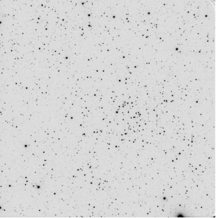
Figure 1: V 60 secs image centered on Berkeley 44. North is up, east on the left. The field is 10 arcmin on a side.

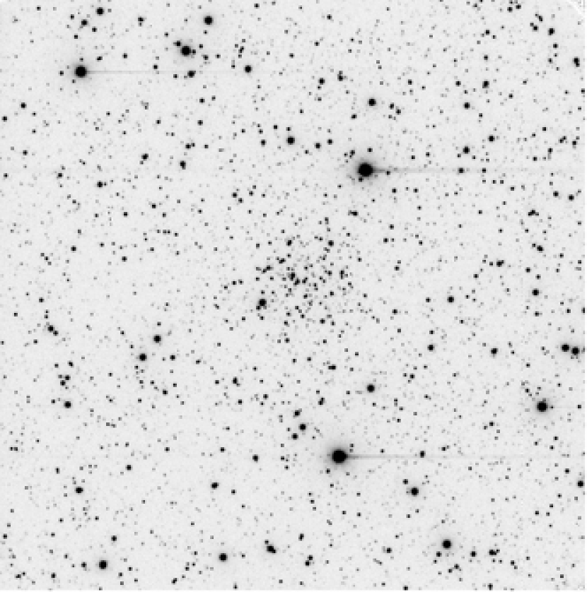
Figure 2: V 60 secs image centered on NGC 6827. North is up, east on the left.

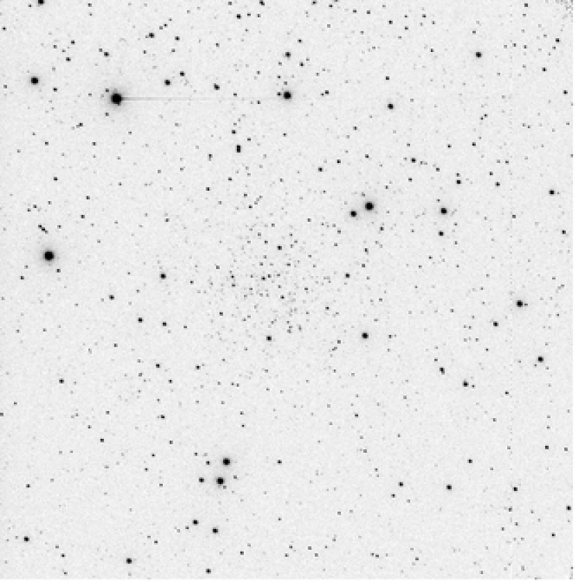
Figure 3: V 60 secs image centered on Berkeley 52. North is up, east on the left.

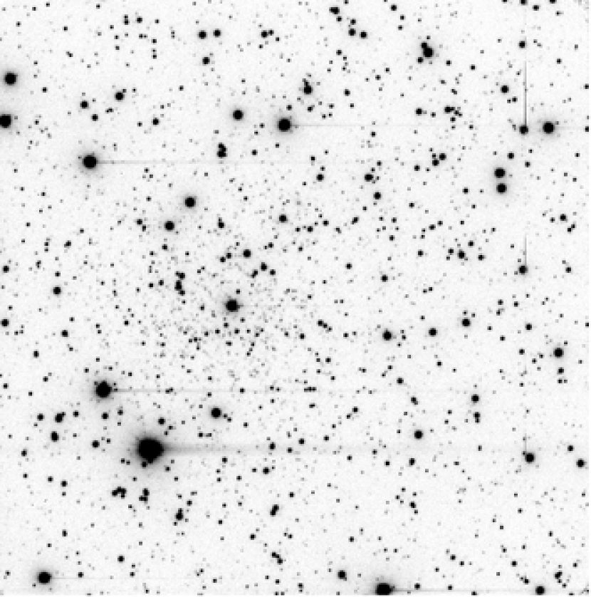
Figure 4: V 60 secs image centered on Berkeley 56. North is up, east on the left.

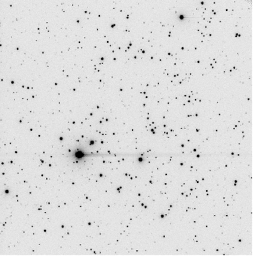
Figure 5: V 60 secs image centered on Skiff 1. North is up, east on the left.

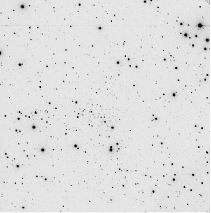
Figure 6: V 60 secs image centered on Berkeley 5. North is up, east on the left.

2 Observations and Data Reduction

The observations were done using the 2-m Himalayan Chandra Telescope (HCT), located at Hanle, IAO and operated by Indian Institute of Astrophysics. Details of the telescope and the instrument are available at the Institute’s homepage (http://www.iia.res.in/). The CCD used for imaging is a 2 K $\times$ 4 K CCD, where the central 2 K $\times$ 2 K pixels were used for imaging. The pixel size is 15 $\mu$ with an image scale of 0.297 arcsec/pixel and the average seeing was 1.3 and 1.4 arsec on August 9 and 30, respectively. The total area observed is approximately 10 $\times$ 10 arcmin². Images of the clusters are presented in Figures 1 - 6.

The data have been reduced with the IRAF packages CCDRED, DAOPHOT, ALLSTAR and PHOTCAL using the point spread function (PSF) method (Stetson 1987).

The nights were photometric and Landolt (1992) standard field SA110 was observed for calibration at different air-masses during the night to put the photometry into the standard system.

Table 2: Log of photometric observations on August 9 and 30, 2005.

Cluster	Date	Filter	Exp time (sec)
Be 44	09 August 2005	V	60, 180, 2X300
		B	2X120, 2X600
		I	2, 5, 10, 2X30, 2X60
Be 44 (Field)		V	60, 2X300
		B	2X600
		I	2, 2X60
NGC 6827	30 August 2005	V	60, 180, 2X300
		B	120, 300, 2X600
		I	10, 30, 60, 2X120
Be 52	09 August 2005	V	60, 180, 2X420
		B	120, 600, 900
		I	10, 30, 120, 300
Be 56	30 August 2005	V	30, 60, 2X180
		B	180, 300, 600
		I	10, 30, 60, 2X120
Skiff 1	30 August 2005	V	20, 60, 2X180
		B	30, 120, 300, 600
		I	10, 30, 60, 120
Skiff 1 (east)		V	30, 180
		B	60, 300
		I	30, 120
Be 5	30 August 2005	V	60, 3X180
		B	60, 300, 600
		I	10, 30, 180, 300

Figure 7: Star counts in the V passband for the clusters under investigation. The dashed lines in the Berkeley 44 and Skiff 1 panels indicate the level of the background as derived from the accompanying control field.

Figure 8: Color Magnitude Diagrams of NGC 6827 (lower panels) and Berkeley 56 (upper panels). Only the stars inside the cluster radius are shown.

Figure 9: Color Magnitude Diagrams of Berkeley 52 (lower panels) and Berkeley 5 (upper panels). Only the stars inside the cluster radius are shown.

Together with the clusters, we observed two control fields, one east of Skiff 1 at 01:06:24, +68:29:00 (J2000.0), and the other north of Berkeley 44 at 19:17:12, +19:38:00 (J2000.0), to deal with field star contamination. In fact these are the only two clusters which seem to extend beyond the field covered by the CCD.

The calibration equations are of the form:

$b=B+b_{1}+b_{2}\times X+b_{3}~{}(B-V)$
$v=V+v_{1}+v_{2}\times X+v_{3}~{}(B-V)$
$i=I+i_{1}+i_{2}\times X+i_{3}~{}(V-I)$ ,

Table 3: Coefficients of the calibration equations: August 9, 2005

$b_{1}=0.803\pm 0.007$	$b_{2}=0.25\pm 0.02$	$b_{3}=-0.043\pm 0.006$
$v_{1}=0.495\pm 0.006$	$v_{2}=0.16\pm 0.02$	$v_{3}=0.063\pm 0.004$
$i_{1}=0.826\pm 0.012$	$i_{2}=0.08\pm 0.02$	$i_{3}=0.044\pm 0.009$

Table 4: Coefficients of the calibration equations: August 30, 2005

$b_{1}=0.818\pm 0.008$	$b_{2}=0.26\pm 0.02$	$b_{3}=-0.043\pm 0.008$
$v_{1}=0.513\pm 0.005$	$v_{2}=0.14\pm 0.02$	$v_{3}=0.063\pm 0.005$
$i_{1}=0.824\pm 0.009$	$i_{2}=0.08\pm 0.02$	$i_{3}=0.048\pm 0.009$

where $BVI$ are standard magnitudes, $bvi$ are the instrumental ones and $X$ is the airmass; all the coefficient values are reported in Tables 3 and 4. The standard stars in these fields provide a very good color coverage being 0.1 $\leq(B-V)\leq$ 2.2 and 0.4 $\leq(V-I)\leq$ 2.6

Aperture correction was then derived from a sample of bright stars and applied to the photometry. We used aperture of 14 pixels for the standards stars and of 7-9 pixels for the science frames, depending on the frame. The average aperture correction amounted at 0.27, 0.29 and 0.20 mag in B,V and I, respectively for the August 9 night, and 0.25, 0.25 and 0.21 for the August 30 night.

Finally, the completeness corrections were determined by artificial-star experiments on our data. Basically, we created several artificial images by adding to the original images artificial stars. About a total of 4000 stars were added to the original images. In order to avoid the creation of overcrowding, in each experiment we added at random positions only 15$\%$ of the original number of stars. The artificial stars had the same color and luminosity distribution of the original sample. This way we found that the completeness level keeps above 50$\%$ down to V = 20.5.

The limiting magnitudes are B = 22.0, V = 22.5 and I =21.5.
The final photometric catalogs for (coordinates, B, V and I magnitudes and errors) consist of 11000, 10525, 12730, 2250, 2973, 7117, and 6486 stars for NGC 6827, NGC 6846, Berkeley 44, Berkeley 5, Berkeley 52, Berkeley 56 and Skiff 1, respectively, and are made available in electronic form at the WEBDA site maintained by E. Paunzen.

3 Star counts and cluster sizes

As a first step in the analysis of the clusters, we performed star counts to obtain an estimate of the cluster radius. This is an important step in order to pick up the most probable cluster members and minimize field star contamination. By inspecting clusters charts we identified the cluster center, and performed star counts in circular annuli 0.5 arcmin wide around the cluster center. In order to increase the contrast, we consider in each cluster only the stars fainter than the clump.
The results are shown in Fig. 7. Here the error bars are the Poisson error of the star counts in each annulus.
In the case of Berkeley 44 and Skiff 1 we estimate the level of the background from the accompanying offset field, and draw it with a dashed line in Fig. 7. By inspecting Fig. 7 the following considerations can be done:

• NGC 6827, NGC 6846, Berkeley 52, Berkeley 56 and Berkeley 5 are compact clusters with radii between 1 and 2 arcmin;

• Berkeley 44 does not show a well-defined outer radius, since star counts fall smoothly along the entire area covered by this study. For this cluster we have observed an offset field (see Sect. 2) which we are going to analyze in the following Section.

• Although there is a visible overdensity of stars in the Skiff 1 region the overdensity suggests the form of a ring structure 2 arcmin from the cluster nominal center. As shown in the following discussion, Skiff 1 is both a sparse cluster and rather more nearby than the other clusters. For this reason we have used a different annulus size (1.0 arcmin) to derive the profile.

Estimates of the cluster sizes, taken from Figure 7, are presented in Table 6; they are in good agreement with the Dias et al. (2002) compilation, which is based on visual inspection.

Figure 10: Color Magnitude Diagrams of Skiff 1 and Berkeley 44. The right panels are the comparison field. Note the anomalous blue MS with a TO at V = 19.5 in the CMD of Skiff 1 and its control field.

Table 5: Preliminary age estimates based on the $\Delta~{}V$ method

$Name$	$V_{T}O$	$(B-V)_{TO}$	$(V-I)_{TO}$	$V_{clump}$	$(B-V)_{clump}$	$(V-I)_{clump}$	$\Delta V$	$Age$
	mag	mag	mag	mag	mag	mag	mag	Gyr
Berkeley 44	17.50$\pm$0.05	1.75$\pm$0.10	2.00$\pm$0.10	16.50$\pm$0.11	2.25$\pm$0.12	2.50$\pm$0.14	1.00$\pm$0.12	1.1$\pm$0.25
NGC 6827	17.50$\pm$0.05	1.20$\pm$0.10	1.40$\pm$0.10	16.75$\pm$0.25	2.00$\pm$0.29	2.15$\pm$0.32	0.75$\pm$0.25	0.8$\pm$0.20
Berkeley 52	20.50$\pm$0.05	2.00$\pm$0.10	2.20$\pm$0.10	19.00$\pm$0.09	2.50$\pm$0.23	2.80$\pm$0.25	1.50$\pm$0.10	1.8$\pm$0.30
Berkeley 56	20.50$\pm$0.05	0.80$\pm$0.10	1.10$\pm$0.10	17.70$\pm$0.08	1.50$\pm$0.16	1.75$\pm$0.18	2.30$\pm$0.09	4.0$\pm$0.50
Skiff 1	15.50$\pm$0.05	1.10$\pm$0.10	1.30$\pm$0.10	14.70$\pm$0.11	1.80$\pm$0.13	2.00$\pm$0.13	0.80$\pm$0.12	0.9$\pm$0.20
Berkeley 5	19.50$\pm$0.05	1.30$\pm$0.10	1.50$\pm$0.10	18.60$\pm$0.17	2.10$\pm$0.21	2.40$\pm$0.23	0.90$\pm$0.18	1.0$\pm$0.20

4 Color Magnitude Diagrams: Are these real clusters?

By using the results of the previous section we generate the CMDs of the clusters considering only the stars within the assumed cluster radius (Table 6). The results are shown in Figs. 8 to 10. All of the clusters are located in crowded galactic plane fields and the CMDs are heavily contaminated with the projected background main sequence population of the galaxy. In spite of this contamination, an apparent red giant clump is noticeable on all of the diagrams. We use this as our first evidence for the existence of physical clusters.

We can improve the contrast between the clusters and the background field by employing a statistical method to clean the CMDs. For each cluster, we selected a field region far from the cluster region. This selection was done in in the same CCD field for all the clusters except Berkeley 44 and Skiff 1, for which we have at disposal an offset field. The cluster and field regions have the same area.

To perform the statistical subtraction, we employed the technique described in Vallenari et al. (1992) and Gallart et al. (2003).
Briefly, for any star in the field, we look for the closest (in color and magnitude) star in the cluster, and remove this star from the cluster CMD. This procedure takes into account the photometric completeness (see Section 2.)
The results are shown in the series of Figs. 11 to 16. In these figures, the left panel shows the CMD for stars inside the selected radius, whereas the mid-left panel shows the offset equal area field. The cleaned CMD is then shown in the mid-right panel. In each case, the cleaning process leaves an apparent cluster CMD; we assume in the remainder that all of these are physical systems.

Finally the isochrone fitting is presented in the right panel (see the next section).

To get a first estimate of cluster age, we now employ the $\Delta V$ (magnitude difference between the TO and the RGB clump) vs age calibration by Carraro $\&$ Chiosi (1994). This method is independent of distance and reddening, and depends only on metallicity. The results are summarized in Table 5 together with their uncentainties. The magnitude and colors of the TO have been estimated by eye, whilst the magnitude and colors of the clump are the mean magnitude and colors of the stars in the clump area in the CMD. Basing on this method all the clusters are of Hyades age or older, with Berkeley 56 being the oldest of the sample.

An inspection of each CMD allows us to derive the following considerations:

NGC 6827. The cluster looks like an intermediate-age one, with a prominent clump of stars at V $\approx$ 16.5 and (B-V) $\approx$2.7, (V-I) $\approx$ 2.1. The Turn Off point (TO) is located at V $\approx$ 17.75, (B-V) $\approx$ 1.0. The MS looks truncated at V$\sim$ 19.5 as a result of the cleaning procedure

Berkeley 52. This is a faint and heavily reddened cluster. The presence of a clear clump witnesses that the cluster is relatively old.

Berkeley 5 This cluster is poorly populated; the clump, if real, is very sparse, which can be a signature of significant differential reddening. The TO however is readily detectable, which ensures the reality of this cluster.

Berkeley 56 It looks a promising old cluster, with a tight clump at V $\approx$ 17.5. The TO area is at the limit of the photometry, although the TO can easily be identified at V $\approx$ 20.

Skiff 1 This is a very interesting object. There is clear clump at V $\approx$ 15, which is not visible in the control field and ensures this is a real intermediate-age/old cluster. We have to note here (both in the cluster and the offset field) the presence of a faint blue population with a TO at V = 19.5. This is similar to the one detected in the third Galactic Quadrant (Bellazzini et al. 2004) and in the second Galactic Quadrant (Bragaglia et al. 2006) and routinely attributed to the Canis Major Galaxy (Bellazzini et al. 2004). This is quite remarkable since this presumed dwarf Galaxy (or its tidal tail) is not expected to extend to this Galactic location (Martin et al. 2004, Fig. 4).

Berkeley 44 The contamination of field stars is severe in this case. However the upper part of the MS and the evolved stars region are significantly more populated than in the control field. We suggest that this cluster is real.

5 Estimates of Fundamental parameters

In order to derive more reliably the cluster fundamental parameters, namely reddening, age and distance, we employ the following technique, using the cleaned CMDs in figures 11 to 16.

Possible isochrone solutions are obtained by exploring a large number of isochrones; for clarity only the isochrone with the best visual match to the observed one is presented. To achieve the best match we paid attention to the slope of the MS, the position and shape of the TO region and the magnitude and color of the RGB clump. These constraints are function of age, metallicity, distance and reddening, and must be reproduced at the same time. Lacking a spectroscpopic estimate of the metallicity, we employ the solar metallicity set.

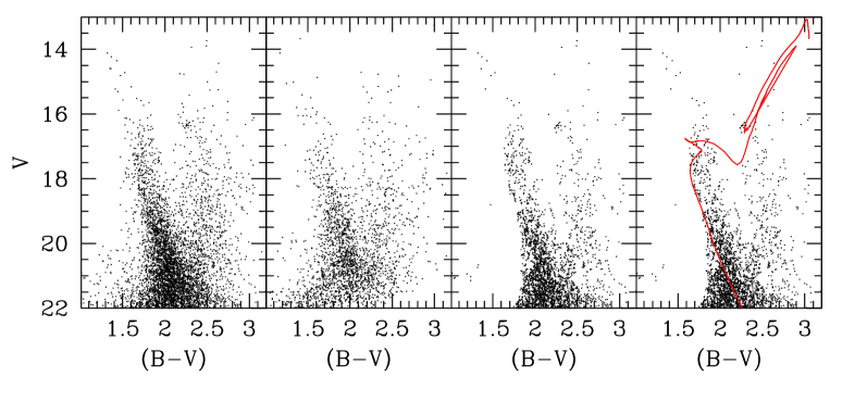
Figure 11: Left panel: CMD of Berkeley 44;Mid-left panel: CMD of the control field; Mid-right panel: the clean CMD; Right panel:Isochrone solution for Berkeley 44: the 1.3 Gyr isochrone is shitfed by E(B-V) = 1.40 en V-M_V = 15.60.

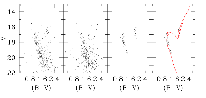
Figure 12: Left panel: CMD of NGC 6827;Mid-left panel: CMD of the control field; Mid-right panel: the clean CMD; Right panel:Isochrone solution for NGC 6827: the 0.8 Gyr isochrone is shitfed by E(B-V) = 1.05 en V-M_V = 16.30

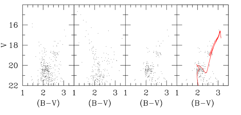
Figure 13: Left panel: CMD of Berkeley 52;Mid-left panel: CMD of the control field; Mid-right panel: the clean CMD; Right panel:Isochrone solution for Berkeley 52: the 2.0 Gyr isochrone is shitfed by E(B-V) = 1.50 en V-M_V = 18.10

The uncertainty in each parameter simply mirrors the degree of freedom we have in displacing an isochrone still achieving an acceptable fit.

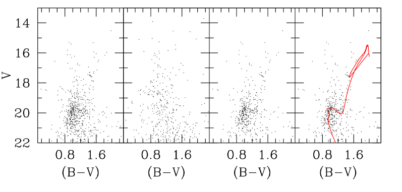
Figure 14: Left panel: CMD of Berkeley 56;Mid-left panel: CMD of the control field; Mid-right panel: the clean CMD; Right panel:Isochrone solution for Berkeley 56: the 4.0 Gyr isochrone is shitfed by E(B-V) = 0.40 en V-M_V = 16.60

The results of the isochrone fitting method are summarized in Table 6, where for each cluster radius, reddening, distance modulus, heliocentric distance, Galactic Cartesian coordinates, Galactocentric distance, and age are reported.
To derive the cluster heliocentric distance we corrected the apparent distance modulus (V-M_V) by adopting the standard ratio of selective to total absorption $R_{V}=\frac{A_{V}}{E(B-V)}=3.1$.

A few comments are in order:

• All the clusters are substantially reddened, with E(B-V) ranging from 0.40 to 1.50;

• all the cluster are older than the Hyades, and therefore they constitute a significant contribution to the old open cluster population in the Galactic disk;

• Two of them lie inside the solar circle, which is a remarkable result, since star clusters are not expected to survive so long in the dense environment typical of the inner part of the Galactic disk;

• they span about 7 kpc in Galactocentric distance, but they do not seem to follow the radial abundance gradient (Carraro et al. 1998); this however has to be considered a preliminary results, due to the really crude estimate of the metallicity we can infer from isochrone fitting.

• the oldest cluster of the sample is Berkeley 56, which also lies high onto the Galactic plane, and it is one of the most distant cluster from the Sun (Friel 1995)

• Berkeley 56 with an age of 4 Gyr falls in an age bin where a minimum in the star cluster age distribution was suggested to exist; however the discovery of several new clusters in this age bin (Carraro et al. 2005) significantly reduces the reality of this minimum, and suggests that the age distribution of old open clusters is simply an e-folding relation.

• the clean CMDs of Berkeley 44, 52 and 56 show the presence of a bunch of stars above the TO. These stars can be field stars that the cleaning procedure was not able to remove, or they can be blue stragglers and binary stars, quite common in clusters of this age.

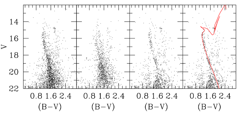
Figure 15: Left panel: CMD of Skiff 1;Mid-left panel: CMD of the control field; Mid-right panel: the clean CMD; Right panel:Isochrone solution for Skiff 1: the 1.2 Gyr isochrone is shitfed by E(B-V) = 0.85 en V-M_V = 13.70

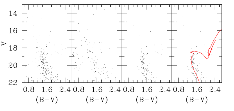
Figure 16: Left panel: CMD of Berkeley 5;Mid-left panel: CMD of the control field; Mid-right panel: the clean CMD; Right panel:Isochrone solution for Berkeley 5: the 0.8 Gyr isochrone is shitfed by E(B-V) = 1.30 en V-M_V = 18.00

6 A closer look at Skiff 1

We now concentrate a bit more on the open cluster Skiff 1. It is a nearby star cluster, and although it is not a rich cluster, among the clusters presented here, the cleaned CMD is the most distinct, with a MS apparently extending for more than 6 mag. This offers the opportunity to better constrain its fundamental parameters and we employ here for this purpose the synthetic CMD technique.
The method is described in detail in Carraro et al. (2002) and Girardi et al. (2005). Briefly, we count the number of clump stars ($\sim$18) , and assign to the cluster a total mass ($1.8\times 10^{3}M_{\odot}$) according to the Kroupa (2001) Initial Mass Function (IMF). A population of binaries is then added, in a 30$\%$ fraction, and with mass ratio between 0.7 and 1.
Then we simulated the effect of the photometric errors, with typical values derived from our observations. The results are shown in Fig. 17, panels a) and c). The age, distance modulus, reddening and metallicity are the ones listed in Table 6.

In order to estimate the location of foreground and background stars we use a Galactic model code (Girardi et al. 2005), and generate the CMD of the Galactic population in the direction of the cluster and within the same cluster area. Again, this CMD is then blurred by adding photometric errors (see panels b) and d) ).

The combination of the simulated cluster and field is then shown in panel e), which must be compared with the observations in panel f).

The close similarity of the simulated and observed CMDs ensures us that the adopted parameters for Skiff 1 are correct within the errors, and confirms the results of the simpler isochrone fitting method.

Moreover it tells us that the Galactic model successfully accounts for the field population toward the cluster. In particular the blue Main Sequence is naturally accounted for by stars belonging to the of halo and thick disk of the Galaxy without any need to invoke an extra-population.

Figure 17: Simulation of Skiff 1 and its field in the V versus B-V diagram. (a) Simulation of a $1.2$-Gyr old cluster with $Z=0.019$ and a initial mass of $1.8\times 10^{3}$ $M_{\odot}$, based on the same isochrones, distance modulus and colour excess as in Table 5. We have assumed that 30 percent of the stars are binaries with mass ratios between 0.7 and 1.0. (b) Simulation of a $10.14\times 10.14{\rm arcmin}^{2}$ field centered at Galactic coordinates $l=123^{\circ}.57$, $b=+5^{\circ}.60$, performed with Girardi et al. (2005) Galactic model. Panels (c) and (d) are the same as (a) and (b), respectively, after simulation of photometric errors. Panel (e) shows the sum of (c) and (d), that can be compared to the observational data shown in panel (f).

7 Discussions and Conclusions

We have presented CCD BVI photometry for 6 previously unstudied possibly old open clusters, namely Berkeley 44, NGC 6827, Berkeley 52, Berkeley 56, Skiff 1 and Berkeley 5.

We have found that all the clusters are actually old, and the ages range from 0.8 to 4 Gyr. This sample of clusters represents an important contribution to the poorly populated old open clusters family in the Galactic disk. In Fig. 18 we show an updated age distribution of the old open cluster (older than 500 Myr) so far known.
This comes from Carraro et al. (2005), where we added the new clusters studied in this paper and Auner 1 (3.5 Gyr, Carraro et al. 2006).

The new age distribution can be easily fitted with an exponential relation having an e-folding time of 2 Gyr. This means than on the average the oldest clusters in the Milky Way do not survive more than 2 Gyr. This estimate is an order of magnitude larger than the typical life-time of an open cluster (200 Myr), and suggests that old open clusters survive longer possibly due to particular situations, like birth-places high onto the Galactic plane, or the preferentially high total mass at birth. It might also possible that some open clusters, especially in the anti-centre could have entered the Milky Way in the past together with cannibalized satellites (Frinchaboy et al. 2004)

Much firmer conclusions might be drawn as additional old clusters are discovered and studied.

Table 6: Parameters of the studied clusters. The coordinate system is such that the Y axis connects the Sun to the Galactic Center, while the X axis is positive in the direction of galactic rotation. Y is positive toward the Galactic anti-center, and X is positive in the first and second Galactic quadrants (Lynga 1982).

$Name$	$Radius$	$E(B-V)$	$(m-M)$	$d_{\odot}$	$X_{\odot}$	$Y_{\odot}$	$Z_{\odot}$	$R_{GC}$	$Age$
	${\prime}$	mag	mag	kpc	kpc	kpc	pc	kpc	Myr
Berkeley 44	$\geq 5.0$	1.40$\pm$0.10	15.6$\pm$0.2	1.8	1.4	-1.1	100	7.6	1300$\pm$200
NGC 6827	1.5	1.05$\pm$0.05	16.3$\pm$0.2	4.1	3.5	-2.1	-170	7.3	800$\pm$100
Berkeley 52	1.5	1.50$\pm$0.10	18.1$\pm$0.2	4.9	4.5	-1.8	-270	8.1	2000$\pm$200
Berkeley 56	1.0	0.40$\pm$0.05	16.6$\pm$0.2	12.1	12.0	-0.8	-1100	14.3	4000$\pm$400
Skiff 1	$\geq$5.0	0.85$\pm$0.05	13.7$\pm$0.2	1.6	1.3	0.9	160	9.5	1200$\pm$100
Berkeley 5	1.0	1.30$\pm$0.10	18.0$\pm$0.2	6.2	4.8	3.9	80	13.3	800$\pm$100

Figure 18: Age distribution of known open clusters older than 500 Myr. The dashed exponential line has an e-folding time of 2 Gyr.

References

- [1] Bellazzini M., Ibata R., Martin N., Irwin M.J., Lewis G.F., 2004, MNRAS 354, 1263
- [2] Bragaglia A., Tosi M., Andreuzzi G., Marconi G., 2006, MNRAS 368, 1971
- [3] Carraro G., Chiosi C., 1994, A&A 287, 761
- [4] Carraro G., Girardi L., Marigo P., 2002, MNRAS 332, 705
- [5] Carraro G., Ng K.Y., Portinari L., 1998, MNRAS 296, 1045
- [6] Carraro G., Geisler D., Moitinho A., Baume G., & Vázquez R.A., 2005, A&A 442, 917
- [7] Carraro G., Moitinho A., Zoccali M., Vázquez R.A., & Baume G., 2006, AJ, submitted
- [8] de la Fuente Marcos R. & de la Fuente Marcos C., 2004, New. Astronomy 9, 475
- [9] Dias W.S., Alessi B.S., Moitinho A., Lepine J.R.D., 2002, A&AS 141, 371
- [10] Friel E.D. 1995, ARA&A 33 , 381
- [11] Frinchaboy P.M., Majewski S.R.; Crane J.D. Reid I. N., Rocha-Pinto H.J., Phelps R. L., Patterson R.J., Munoz R.R., 2004, ApJ 602, L21
- [12] Gallart C., Zoccali M., Bertelli G., Chiosi C., Demarque P., Girardi L., Nasi E., Woo J.-H., Yi S., 2003, AJ 125, 742
- [13] Girardi L., Bressan A., Bertelli G., Chiosi C., 2000, A&AS 141, 371
- [14] Girardi L., Groenewegen M.A.T., Hatziminaoglou E., da Costa L., 2005, A&A 436, 895
- [15] Hasegawa T., Malasan H.L, Kawakita H., Obayashi H., Kurabayashi T., Nakai T., Hyakkay M., Arimoto N. 2004, PASJ 56, 295
- [16] Kroupa P., 2001, MNRAS 322, 231
- [17] Landolt A.U., 1992, AJ 104, 340
- [18] Lynga G., 1982 A&A 109, 213
- [19] Luginbuhl C., Skiff B., 1990, Observing Handbook and Catalogue of Deep-Sky Objects, Cambridge Univ Press
- [20] Martin N., Ibata R., Bellazzini M., Irwin M.J., Lewis G.F., Denhen W., 2004, MNRAS 348, 12
- [21] Ortolani, S., Bica, E., Barbuy, B., & Zoccali, M., 2005 A&A 429, 607
- [22] Phelps, R.L., Janes, K.A., Montgomery, K. A., 1994, AJ 107, 1079
- [23] Setteducati A.E., Weaver M.F., 1960, in Newly found stellar clusters, Radio Observatory Lab., Berkeley
- [24] Stetson, P., 1987, PASP 99,191
- [25] Vallenari A., Chiosi C., Bertelli G., Meylan G., Ortolani S., 1992, AJ 104, 1100
- [26] Wielen R., 1971, A&A 13, 309