A Catalog of Spectroscopically Confirmed White Dwarfs from the Sloan Digital Sky Survey Data Release 4

Abstract

We present a catalog of 9316 spectroscopically confirmed white dwarfs from the Sloan Digital Sky Survey Data Release 4. We have selected the stars through photometric cuts and spectroscopic modeling, backed up by a set of visual inspections. Roughly 6000 of the stars are new discoveries, roughly doubling the number of spectroscopically confirmed white dwarfs. We analyze the stars by performing temperature and surface gravity fits to grids of pure hydrogen and helium atmospheres. Among the rare outliers are a set of presumed helium-core DA white dwarfs with estimated masses below $0.3\rm M_{\odot}$, including two candidates that may be the lowest masses yet found. We also present a list of 928 hot subdwarfs.

Astrophysical Journal Supplements, in press

1 Introduction

The Sloan Digital Sky Survey (SDSS) is greatly expanding the number of spectroscopically confirmed white dwarf stars. Harris et al. (2003) presented a catalog of 269 white dwarfs from the Early Data Release, and Kleinman et al. (2004) followed this with a catalog of 2551 white dwarfs from SDSS Data Release 1. More specialized SDSS catalogs have been presented for magnetic white dwarfs (Schmidt et al., 2003; Vanlandingham et al., 2005), white dwarf plus M star binary systems (Raymond et al., 2003; Smolĉić et al., 2004; Silvestri et al., 2005), and cataclysmic variables (Szkody et al., 2002, 2003a, 2004, 2005). The size of the SDSS white dwarf catalog has significantly expanded samples of rare white dwarfs, including ultra-cool white dwarfs (Harris et al., 2001; Gates et al., 2004; Kilic et al., 2005), stars with atomic carbon and oxygen (Harris et al., 2003; Liebert et al., 2003), pulsating DAV stars (Mukadam et al., 2004; Mullally et al., 2005) and DBV stars (Nitta et al., 2005), hot DO stars (Krzesiński et al., 2004), very low accretion rate magnetic cataclysmic variables (Szkody et al., 2003b), low-mass degenerate helium core stars (Liebert et al., 2004), and hot DB stars in the “DB gap” (Eisenstein et al., 2005).

Here we present a catalog of white dwarfs and hot subdwarf stars from the SDSS Data Release 4 (Adelman-McCarthy et al., 2006), which presents 800,000 spectra from 4783 square degrees. We use automated techniques supplemented by visual classification to select 13,000 candidates. An extensive analysis of these objects yields 9316 white dwarfs (WD), including 8000 DAs, 713 DBs, 41 DOs or PG1159 stars, 289 DCs, 104 DQs, and 133 DZs. We find 928 hot subdwarf stars (SD), building on the samples from Harris et al. (2003) and Kleinman et al. (2004). We fit the WDs to grids of model atmospheres and present temperatures and surface gravities of the DA and DB stars. We also present 774 duplicate spectra of WDs and 60 duplicate spectra of SDs.

This catalog is not complete, even within the SDSS spectroscopic sample, as we have intentionally focused on the “easy” white dwarfs, namely those that fall in the blue color region of DA and DB stars. Low temperature stars that fall too near the colors of A and F stars have not been searched. Cataclysmic variables have been excluded, as they have been separately cataloged. White dwarf plus M star binaries are included where easily identified, but the catalog of Silvestri et al. (2005) is more complete and better analyzed. Magnetic WDs are sufficiently heterogeneous to fool our automated techniques, but we include them where possible. DC stars are difficult to positively identify, although we do find a fair number.

Although completeness was not our goal, we expect that the catalog does include nearly all of the SDSS white dwarf spectra for the common classes of hotter DA, DB, and DO. We have attempted to find DQ and DZ stars, although this effort is often limited by the signal-to-noise ratio of the spectra.

2 The SDSS

The SDSS (York et al., 2000; Stoughton et al., 2002; Abazajian et al., 2003, 2004; Finkbeiner et al., 2004; Abazajian et al., 2005a; Adelman-McCarthy et al., 2006) is surveying $10^{4}$ square degrees of high-latitude sky in 5 bandpasses: $u$, $g$, $r$, $i$, and $z$ (Fukugita et al., 1996; Gunn et al., 1998, 2006). The images are processed (Lupton et al., 2001; Stoughton et al., 2002; Pier et al., 2003) and calibrated (Hogg et al., 2001; Smith, Tucker et al., 2002; Tucker et al., 2005) to produce 5-band catalogs, from which galaxies (Eisenstein et al., 2001; Strauss et al., 2002), quasars (Richards et al., 2002), and stars are selected for follow-up spectroscopy. Spectra covering 3800Å to 9200Å with resolution of 1800 are obtained with twin fiber-fed double-spectrographs.

The SDSS has obtained many spectra of white dwarfs and other blue stars (Harris et al., 2003; Kleinman et al., 2004) due to a variety of target selection catagories. See Harris et al. (2003) and Kleinman et al. (2004) for further discussion, plots of white dwarfs in SDSS color space, and representative spectra. We will discuss the completeness of the spectroscopic targeting in § 5.6.

In addition to the standard survey spectroscopy, DR4 includes spectra from the special programs that have been executed over the course of the survey. Most of these focus on the equatorial stripe in the South Galactic Cap. We have included these spectra in our search as well. See Adelman-McCarthy et al. (2006) for descriptions of the programs. Some programs, being focused on blue stars or quasars, are reasonable hunting grounds; others have negligible yield. The special programs are indicated by setting the leading bit of the targeting flags.

The SDSS photometric zeropoints are close to the AB convention (Fukugita et al., 1996), but do not reproduce it exactly. We quote all of our photometry on the SDSS system rather than the AB system. However, when fitting models, we do include the following AB corrections: $u_{\rm AB}=u_{\rm SDSS}-0.040$, $i_{\rm AB}=i_{\rm SDSS}+0.015$, $z_{\rm AB}=z_{\rm SDSS}+0.030$, with no correction in $g$ and $r$. These corrections were derived from comparison to the HST STIS spectrophotometric calibration stars (Bohlin et al., 2001) as well as from analysis of the colors of DA white dwarfs in the SDSS. We note that of these corrections, only the $u$-band one matters for any of the WD fitting. The reason for the $u$ band discrepancy has been identified: the definition of the zeropoint in (Fukugita et al., 1996) did not include the effects of atmospheric absorption on the shape of the response function. The AB corrections remain uncertain at least at the 1% level; we are continuing to work on this issue.

3 Catalog Selection and Inspection

3.1 Initial Selection

White dwarfs hotter than roughly 8000 K are distinct in SDSS colors from the much larger samples of galaxies, quasars, and F stars that the SDSS targets for spectroscopy. The primary exception are the white dwarfs with late-type companions, which still remain distinct from the stellar locus in color, albeit in a different region.

Therefore, we begin with a color selection of all objects with SDSS spectroscopy that have $u<21.5$ and colors in one of the following two regions:

$$-2<u-g<0.833-0.667(g-r),$$ (1)

$$-2<g-r<0.2$$ (2)

or

$$0.2<g-r<1,$$ (3)

$$|(r-i)-0.363(g-r)|>0.1,$$ (4)

$$u-g<0.7{\rm\ or\ }u-g<2.5(g-r)-0.5.$$ (5)

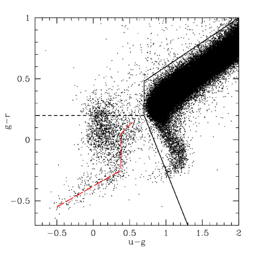
Figure 1: The $u-g$ and $g-r$ colors, dereddened, of blue point sources with clean photometry from about 200 square degrees of the SDSS. The black solid and short-dashed lines show our selection regions, described in § 3.1. The red long-dashed line shows the approximate location of the DA color locus. The region of dense points is the main sequence, extending blueward in $g-r$ to the upper main sequence and blue horizontal branch, before turning blueward in $u-g$ and extending (at much lower densities) toward the hot subdwarfs (shown in Figure 4). The cloud of objects at blue $U-g$ and $g-r\sim 0.2$ are mostly quasars.

The first box selects all of the stars that are bluer in $g-r$ than the quasars and bluer in $u-g$ than the main sequence A stars. The second box runs blueward of the stellar locus in $u-g$ at moderate $g-r$, in order to find WD+M stars. Note that we require that the color not fall on the stellar locus in $g-r$ and $r-i$; this will result in some incompleteness. Figure 1 shows the selection region in $u-g$ and $g-r$ colors relative to the main stellar locus. All of these magnitudes are PSF photometry, dereddened in full from the Schlegel et al. (1998) extinction map. This may overcorrect stars that are in front of some of the Galactic dust, but this has the preferred tendency to bring nearby objects into the sample. We excluded all regions with $r$-band extinction above 0.6 ($A_{g}>0.827$ mag); this removes only a few low-latitude plates outside of the survey region.

We further require that the object pass at least one of the following three cuts based on the two SDSS redshift pipelines (specBS and spec1d). 1) For specBS, we require $|z|<0.003$ and that the classification not be that of a galaxy. 2) For spec1d, we require that zwarning bit 1 not be set and additionally that no band of photometry be flagged as Interp_Center, CR, Edge, or Satur (Stoughton et al., 2002). 3) Alternatively, objects could enter the sample from spec1d if their redshift was greater than 0.003, the photometry flags were not set, and their proper motion from USNO-A was greater than $0.3^{\prime\prime}$ per year. The photometry flags were not checked in option 1, nor was the object required to be a point source. Unfortunately, due to data availability at the time, options 2 and 3 were only queried for point sources in Data Release 3. Option 1 supplied 12904 candidates. Options 2 and 3 supplied another 978 new candidates, for a total of 13882. When restricted to the DR4 region, we analyzed 13641 candidates. 1028 of these were duplicates, which we excluded from the primary analysis.

This selection will not capture all of the white dwarfs in the SDSS spectroscopic catalog, but instead focuses on the regions that include most of the spectroscopic WDs. The obvious failure modes are as follows. 1) White dwarfs cooler than about 8000 K are sufficiently close to the stellar locus that we have not attempted to dig them out. The SDSS photometry is of sufficient quality to cut closer than we have here, but our automated spectral analyses suffer enough at low temperatures that we would have to check many thousand candidates by eye. 2) White dwarfs in binaries with brighter companions can have colors more typical of the stellar locus and hence avoid our selections. 3) Rare classes of white dwarfs may have been given a non-zero redshift by the spectroscopic pipelines if they do not match any of the spectral templates. For example, magnetic WDs can often fool the pipelines. We actually do recover many magnetic WDs, but we are likely not complete. DC white dwarfs also can be dropped from the catalog if the pipelines interpreted a weak noise feature as a low-confidence extragalactic redshift. 4) DC white dwarfs are difficult to confirm in any case.

Our view is that the cooler WDs, being spectroscopically more complicated, are better suited to proper motion analyses. These are being pursued by Harris et al. (2005) and Kilic et al. (2005). Similarly, the WD+M pairs are being cataloged by Silvestri et al. (2005).

3.2 Spectroscopic Analysis

Thus far, we have only selected blue stars, not white dwarfs. We next fit the 13641 candidates to a grid of white dwarf atmospheres using the autofit method described in full in Kleinman et al. (2004). This separates white dwarfs from lower gravity stars.

In brief, the autofit method performs a $\chi^{2}$ minimization of the spectrum and photometry of each candidate relative to a model atmosphere grid, thereby yielding a temperature and surface gravity estimate as well as a classification of helium or hydrogen atmosphere. We use two sets of atmospheres provided by D. Koester (Finley et al., 1997), one pure hydrogen, the other pure helium. Both are computed assuming local thermodynamic equilibrium (LTE) populations. The hydrogen atmospheres run from 6000 K to 100,000 K and $\log g=5.0$ to 9.0. The helium atmospheres run from 10,000 to 40,000 K and $\log g=7.0$ to 9.0. All model spectra are convolved to the spectral resolution of the SDSS data.

The $\chi^{2}$ statistic includes both spectral and photometric residuals. We include the spectrum from 3900Å to 6800Å. The spectral continuum is controlled by marginalizing over an unknown polynomial of 5th order that multiplies the model spectrum. We run autofit on the observed, not dereddened spectra, but this order of polynomial is sufficient to be completely degenerate with the uncertain reddening or with any residual effect of atmospheric dispersion at the fiber entrance. The photometric fit marginalizes over the distance to the star and over extinction values ranging from zero to the Schlegel et al. (1998) prediction, with penalities increasing thereafter. We apply the AB zeropoint corrections described in § 2. Masked pixels in the spectrum are excluded, as are any photometric bands with suspicious warning flags. The star is designated as a hydrogen or helium star based on the best-fit $\chi^{2}$ in the two grids. Errors on the fitted parameters are computed by taking moments of the likelihood function $\exp(-\chi^{2}/2)$ within the chosen grid.

We find that the autofit temperatures and surface gravities do a credible job, even unsupervised, of distinguishing between white dwarfs and other types of stars. This is shown in Figures 2 and 3, which show the distribution of temperatures and gravities of the hydrogen and helium stars that were in the DR1 WD catalog (Kleinman et al., 2004). The visual classification from Kleinman et al. (2004) is shown in the two panels of Figure 2 and in the point type in Figure 3. The separation of the white dwarf locus is clear. Subdwarfs tend to fall at low gravity and moderate temperatures; F and A stars fall to the low temperature extreme. Other weak line stars and CVs fall at low temperatures, particularly in the helium grid, where the model lines are very weak. Notably, DZ, DC, and DQ stars often migrate to low fitted temperatures; the next section will describe how we attempt to recover these stars.

We therefore designate regions in the temperature-gravity space to indicate our first-pass classification. These regions are drawn in Figures 2 and 3. The high-temperature, high-gravity region are called DA and DB, respectively; the high-temperature/low-gravity region are hot subdwarf candidates; and the low-temperature region are left as unknown.

3.3 Inspections

We then subject these classifications to a large series of additional tests. Failing these tests leads to visual examination, which can reject the object as a white dwarf, alter its classification, or rescue it back from the unknown pile.

Several of these tests involve searching for anomalous spectral features. We do this by defining narrow windows at the relevant wavelength and measuring the equivalent width of the residuals of the spectrum relative to the best-fit model (i.e. we use the model to define the continuum rather than interpolating between from neighboring windows). We also estimate the statistical error in the equivalent width using the quoted spectral errors. This ignores the contribution of fluxing errors to the scatter, but this approach is conservative. In this manner, we search for HeI 4471, HeII 4686, $H\alpha$, $H\beta$, CaII 3931, Mg b, and the $C_{2}$ Swan band at 5175 Å.

For the first-pass DA stars, we flag any object whose $\chi^{2}$ from the photometry alone exceeds 50 (on 3 degrees of freedom). These are often DA+M stars, where the $i$ and $z$ photometry is far redder than the blue WD fit. We then search for HeI 4471, HeII 4686, and Swan in emission or absorption and for Mg b or CaII 3931 in absorption; these can find DZ, DQ, DAB, DAO, and CV stars as well as subdwarfs. We flag any star with $\log g<7$ or $T>84,000$ K, as well as $\log g>8.9$ and $T>10,000$ K, as these outliers are suspicious. We flag stars that had reduced $\chi^{2}$ greater than 1.5, or signal-to-noise ratio (SNR) less than 2 per spectroscopic pixel, or 2 or fewer bands of good photometry. We also flag stars with SNR above 4 whose $\chi^{2}$ in the helium and hydrogen fits differ by less than 5%.

The approach is the same for the first-pass DB stars, but we search for $H\alpha$ and $H\beta$ in absorption instead of HeI 4471. After finishing these higher priority inspections, we continued and inspected all of the first-pass DB stars.

For the first-pass hydrogen subdwarfs, we flag stars with gravities above 6.0, as these might be DO stars. For the first-pass helium subdwarfs, we flag those that lack $H\alpha$ and $H\beta$ detections, as these might be misclassified DB stars. We further inspected all of the subdwarfs with $u-g<0.2$, again to look for DO stars.

For the first-pass hydrogen unknowns, our goal is to recover DA+M stars. There are large numbers of F and A star contaminants that tend to pin against the grid extremes in temperature and gravity. We inspect stars that lie away from the edge of the grid. We also flag stars if they have a jump in their spectrum at 8100 Å, as this might signal an M star.

The first-pass helium unknowns are an interesting set because the lowest temperatures in the helium grid have no absorption lines, so any stars without H or He I absorption end up here. We flag stars with $H\alpha$ and $H\beta$ in emission; these are often CVs. We flag stars with Ca II in absorption to find DZs and Swan bands to find DQs.

This selects about 3000 stars for visual inspection, some of which were already inspected in Kleinman et al. (2004). The visual classification of these stars is given in the catalog. However, given the size and heterogeneity of the sample, it is inevitable that there will be errors and uncertainty in the visual classifications too, particularly among certain difficult boundaries.

We expect that the stars that are not visually inspected are a reasonably pure sample, but inevitably some mistakes will have crept in. Figures 2 and 3 show the stars not selected for inspection that overlap with the Kleinman et al. (2004) sample. The DA and DB loci are very pure, and we expect that we have found most of the isolated DA, DB, and DZ stars above 10,000 K in the SDSS spectroscopic sample. Our selection has not been tuned to WD+M binaries and we have lost these stars both in the photometric selection and the spectroscopic classification.

We find that the searching for anomalous emission and absorption has produced sizable lists of DZ, DQ, DAB, DAO, CV, and magnetic WD stars, but we have not made any assessment of the completeness of these samples.

Our catalog of hot (sdB/sdO) subdwarfs is likely reasonably complete, but we have not inspected it to remove interlopers. The temperatures and gravities from autofit surely correlate with the true values, but they are inaccurate because we have not used mixed hydrogen/helium atmospheres. We present the fitted parameters only as a secondary aid to sorting through the catalog. Importantly, our dividing line between the subdwarf list and the unknown list was not drawn to match a robust temperature scale nor to match any particular visual classification standard. Hence, the subdwarf sample should not be used for statistical work without further analysis of the temperature scale and completeness.

At temperatures below 10,000 degrees, the Balmer lines in DA white dwarfs become rather narrow, and it becomes difficult to distinguish between such stars and cooler subdwarfs and blue horizontal branch stars. Normally, the strength of the higher Balmer lines would be used as a surface gravity diagnostic, but this is not always possible because the SDSS spectra become noisy toward the UV. There are likely some DA stars that have been misclassified as subdwarfs and horizontal branch stars, and vice versa.

Similarly, distinguishing between helium-dominated subdwarfs and DB white dwarfs can be subtle, particularly in low signal-to-noise ratio spectra. One can expect a small level of misclassification. However, we have visually inspected all of the DB stars, and are confident that any contamination is small.

4 Classification Schemes

Our visual classifications are based on the systems presented in Harris et al. (2003) and Kleinman et al. (2004). We classify white dwarfs in the standard way as DA, DB, DC, DH, DO, DQ, and DZ. If secondary lines are present, we attach a second letter. For example, a DAB would have dominant hydrogen lines and weaker neutral helium lines.

In all cases, a colon indicates uncertainty in the classification. We use a space to indicate when the uncertainty should be applied only to a portion of the classification. For example, “DA H:” would mean a DA star with possible magnetic contributions, while “DAH:” means that even the DA portion is not firm. We note in particular that by “DBA:” and “DAB:” we are expressing uncertainty with the interpretation as a white dwarf (as opposed, usually, to a hot subdwarf). We write “DB A:” and “DA B:” if we mean that only the presence of the secondary lines is uncertain.

We write “DQhot” to indicate that the carbon lines are atomic rather than molecular (Harris et al., 2003; Liebert et al., 2003). Some of these stars, e.g., SDSS J220029.08-074121.5, are hot enough to show once-ionized carbon, similar to some of the stars in Liebert et al. (2003).

We write “PG1159” to indicate a hot star that is showing highly ionized lines of carbon and oxygen. We have included these as white dwarfs, although these stars are known to span a range of gravities and the evolutionary tracks are continuous between the hottest subdwarfs and hot white dwarfs.

DC stars are generically hard to classify securely. In cases where SDSS has a reasonably high signal-to-noise ratio featureless spectrum with no radio or X-ray counterpart from the FIRST and ROSAT surveys and the object has a statistically significant proper motion, then we assign the star a DC classification. However, the SDSS has many examples of stars with noisier spectra where weak features might be missed. If a star had a significant proper motion and lacked a radio or X-ray counterpart and if the spectrum looked encouragingly but not convincingly featureless, we assigned a DC: classification. The DC: class is likely more permissive than what we would require of a DA: or DB:, but we didn’t want to lose these stars from WD consideration. Further, at low signal-to-noise ratio, the recovery of white dwarfs is surely biased away from DCs and toward white dwarfs with strong features. This bias should be recognized in statistical studies. Likely it can only be avoided by using a reasonably high signal-to-noise ratio or magnitude cut, so as to try to give definitive identifications to nearly all stars.

In this catalog, we have written nearly all companion stars as simply “+M”. Although the companion is almost certainly a dwarf, we have not written “dM”. We have not rigorously typed the star to be a M star. Indeed, sometimes the evidence for the companion is merely emission; we have not indicated such. A colon indicates that the evidence for the companion is not secure. We refer the reader to the paper by Silvestri et al. (2005) for a complete treatment of WD+M binaries, including finer classification, joint parameter fits, and detailed searches for emission. The Silvestri et al. (2005) classifications are to be preferred to our simple “+M” scheme.

For the hot subdwarfs, we have sorted the stars into three classes: SDO, SDB, and Helium-rich SDB (“HeSDB”). However, we caution that our classification has not been particularly systematic. The SDSS hot subdwarfs would benefit from a more quantitative classification scheme, e.g., following Jeffery et al. (1997).

For some of the hot subdwarfs we write “+MS” to indicate a main sequence companion; hot subdwarfs are luminous enough to hold their own with a F or G star, rather than merely a late-type star. However, this classification is very incomplete. As discussed below, the $u-g$ vs. $g-r$ diagram reveals a clear second locus of classified subdwarfs that is clearly due to companions, but we have not been systematic in applying this information.

The automatic classifications are limited to the typing: DA, DB, SD, or other. We add the word “auto” to the classification if a human has not confirmed the classification. There is no binary statement of uncertainty; rather, we refer the user to the temperature and surface gravity values and errors. Obviously, large errors can indicate uncertainty not just in the parameters but in the basic interpretation. This is particularly true in the case of surface gravity. The errors on the temperature are sometimes quite large because the fit is straddling the instability strip and has two local minima (i.e., DA3 and DA5). This does not call the DA interpretation into doubt, but merely indicates that the temperature is uncertain.

Finally, it should be noted that SDSS spectroscopy extends to rather low flux levels ($g\approx 20.5$) and the spectral signal-to-noise ratio of the faintest objects is too poor (as low as 3 per spectroscopic pixel) to permit robust classification. We have attempted to indicate this uncertainty with colons and with the quoted autofit errors. But clearly there will be a strong magnitude and signal-to-noise ratio bias in the recovery of secondary features.

5 Catalogs

5.1 General Properties

We present the catalogs as two tables, one for white dwarfs, the other for hot subdwarfs. The tables include the classifications, the identification information for both imaging and spectroscopy, the photometry, astrometry, and autofit information. The catalog format is given in Table A Catalog of Spectroscopically Confirmed White Dwarfs from the Sloan Digital Sky Survey Data Release 4 but the lines are too long to give in-print samples.

A listing of the classifications, along with the number of stars in each, is given in Tables A Catalog of Spectroscopically Confirmed White Dwarfs from the Sloan Digital Sky Survey Data Release 4, A Catalog of Spectroscopically Confirmed White Dwarfs from the Sloan Digital Sky Survey Data Release 4, and A Catalog of Spectroscopically Confirmed White Dwarfs from the Sloan Digital Sky Survey Data Release 4. Table A Catalog of Spectroscopically Confirmed White Dwarfs from the Sloan Digital Sky Survey Data Release 4 is simply a summary of the dominant classification, meaning the first two letters ignoring any secondary information. The full diversity of classifications are in A Catalog of Spectroscopically Confirmed White Dwarfs from the Sloan Digital Sky Survey Data Release 4 and A Catalog of Spectroscopically Confirmed White Dwarfs from the Sloan Digital Sky Survey Data Release 4. Although mixed typed stars are rare, the size of the DR4 catalog does yield a significant number of them, with many different permutations of the types. For example, there are 16 of the interesting DZA and DAZ stars (Dupuis et al., 1992; Zuckerman & Reid, 1998; Zuckerman et al., 2003; Koester et al., 2005), with 5 uncertain cases and 11 DBAZ/DBZA/DZBA stars.

Figure 4 shows the $u-g$ versus $g-r$ distribution of the stars in the different dominant classifications. As expected, the DA stars have a bent locus due to the strong Balmer break at intermediate temperatures, while the helium-dominated atmospheres follow a more linear locus close to that of a blackbody. The WD+M stars scatter redward in $g-r$ from the single-star locus. It is worth noting that the single star loci end at the dashed line at $g-r=0.2$ rather than the solid line that indicates the boundary of our selection region. This is because at $g-r>0.2$ our selection requires that the star be off of the main sequence color locus in $g-r$ vs. $r-i$. This cut is satisfied by the binary stars but not the single stars. We will postpone discussion of the subdwarf panel until § 7.

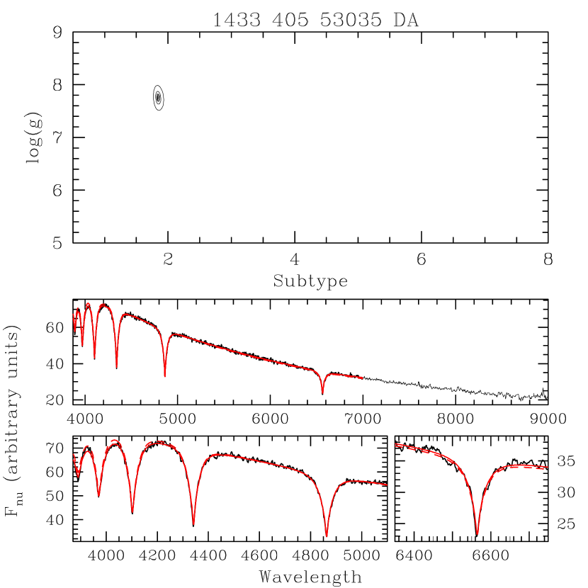
Figure 5: The spectrum and autofit model for the DA star SDSS J104419.00+405553.0 (plate 1433, fiber 405, MJD 53035). This star is unusually bright ($g=16.83$) and high S/N (38 per spectroscopic pixel in the $g$ band). The middle panel shows the full spectrum; the lower panels show expanded views of the Balmer lines. The data is in black. The dashed red line is the best-fit model. The solid red line is the best-fit model having been adjusted by the low-order polynomials that represent reddening and fluxing errors. The top panel plot the likelihood contours for the autofit modeling ($\Delta\chi^{2}$ corresponding to 1, 2, 3, 5, and 10-$\sigma$ for a two-dimensional Gaussian). The DA label at the top is not the classification, but merely the statement that this fitting is for a hydrogen atmosphere.

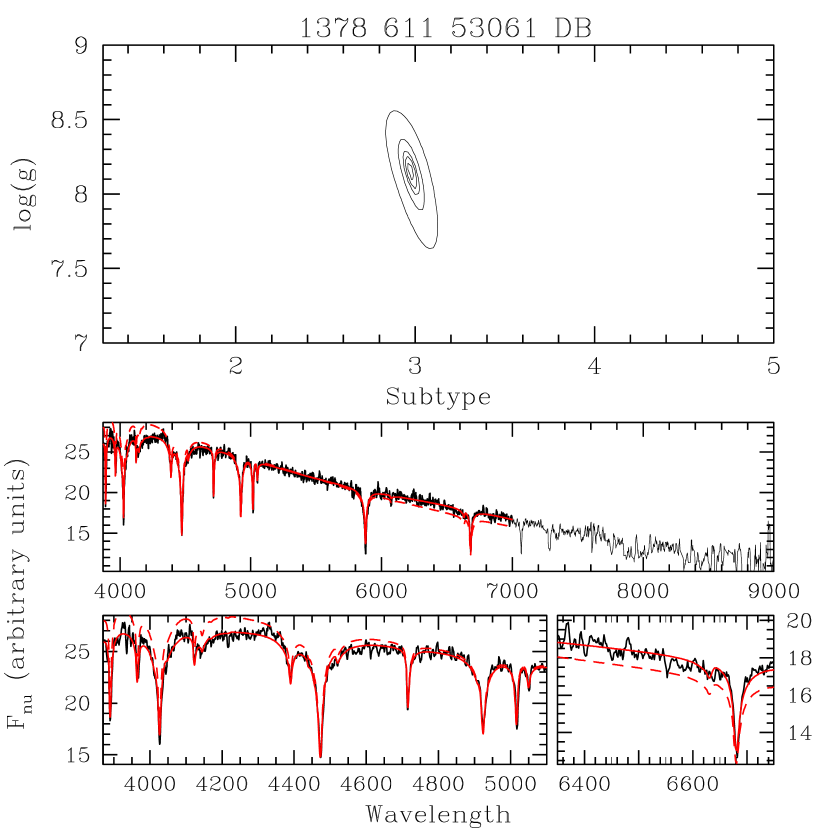
Figure 6: The spectrum and autofit model for the DB star SDSS SDSS J140227.19+403922.2 (plate 1378, fiber 611, MJD 53061). This star is unusually bright ($g=17.78$) and the spectrum has a high S/N ratio (29 per spectroscopic pixel in the $g$ band). The lines and panels are the same as Figure 5. The DB label at the top is not the classification, but merely the statement that this fitting is for a helium atmosphere.

The spectra themselves are available from the SDSS Data Release web site. Each autofit model generates a summary figure, showing the spectrum, the best fit, and the likelihood contours in temperature and surface gravity. These figures are available on-line; examples of a bright DA and bright DB are shown as Figures 5 and 6. The best-fit model is shown in the red dashed line. The red solid line shows the model modified by a multiplicative 5^th-order polynomial. Typically some modification is appropriate to account for extinction or spectrophotometry residuals. The spectra themselves are shown as observed, not dereddened, so it is quite common for the spectrum to be somewhat redder than unextincted model. However, if the broadband model is very different than the data, or the modified model is a poor fit to the data, then this is of course a warning that the autofit parameters are not trustworthy.

In table A Catalog of Spectroscopically Confirmed White Dwarfs from the Sloan Digital Sky Survey Data Release 4, we list the stars from the SDSS DR1 white dwarf catalog of Kleinman et al. (2004) that did not make the list here. There are 73 such stars, about 3% of the Kleinman et al. (2004) sample. These stars are missing not because we doubt their classification but because they did not pass our initial selection cut. In a few cases, this is because the extinction was large or because the photometry was bad. Some of the low temperature stars or binary systems simply didn’t pass our color cuts. The primary reason, however, was that the system was not identified as being at redshift $|z|<0.003$ by either pipeline. This is common in the case of DC stars, when the pipeline may interpret a weak noise feature as a extragalactic redshift, even if it reports it as low confidence. There are about a dozen normal WDs that fool the pipeline as well. For this work, we did not inspect every extragalactic redshift for a blue point source, even those at low confidence. There are many quasars that satisfy those cuts, and we chose not to devote that much effort to rectify a small incompleteness. Future catalogs might find reasonable paths around this, particularly by working with the QSO catalog team (Schneider et al., 2005).

In 52 cases, DR4 includes a spectrum of a white dwarf without the relevant photometry. We have chosen to include these objects in the catalogs despite the missing information. In most cases, the star is part of a special program or a bonus plate located outside of the nominal survey area; such imaging was not included in DR4. In the few remaining cases, the star was blended with other nearby objects in such a way that it was recovered and targeted in a early version of the photometric reductions but not identified as a separate object in later reductions and hence missed in the astrometric matching.

We have matched our catalog to the listing of literature white dwarfs compiled by McCook & Sion (1999) (updated as of August 2005). We find 2343 matches. However, 2179 of these matches were published in the SDSS DR1 white dwarf catalog (Kleinman et al., 2004), which was then incorporated into the updated McCook & Sion (1999) list. Only 162 of the matches are to stars that were not in Kleinman et al. (2004). In total, the DR4 catalog includes 6159 white dwarfs that were not in Kleinman et al. (2004), Silvestri et al. (2005), or the McCook & Sion (1999) list, although it is possible that a handful of these stars are already in the literature. As this number is slightly more than the total in the McCook & Sion (1999) list, we have slightly more than double the world’s list of spectroscopically confirmed white dwarfs.

In 9 cases matched to the McCook & Sion (1999) list, we classified the spectrum as a subdwarf: SDSS J074010.50+284120.8 (WD0737+288), SDSS J082802.03+404008.9 (WD0824+408), SDSS J095847.23+602147.2 (WD0955+606), SDSS J102234.91+460058.7 (WD1019+462), SDSS J122711.17+003328.8 (WD1224+008), SDSS J152553.46+434127.7 (WD1524+438), SDSS J153411.09+543345.3 (WD1532+547), SDSS J154338.68+001202.1 (WD1541+003), and SDSS J233541.46+000219.4 (WD2333-002). These 9 have been eye-inspected to confirm the rejection of the white dwarf interpretation.

5.2 Autofit Results

We have included the fitted temperatures and gravities for all stars in the catalog. However, we stress that these values are only to be used if the classification is DA or DB (possibly with colons), without more subtle variations. If the classification is more complicated, then this almost surely means that the atmosphere is more complicated than the simple pure hydrogen and pure helium values used in autofit. Using the wrong atmosphere grid (e.g., fitting DBA or DZA stars as a DA) can produce catastrophically wrong results. Similarly, in cases where the stars lack Balmer or neutral helium lines, the method will have fit to the models with the weakest lines, typically low temperature and high gravities. This quality assurance decision is recorded in the catalog by the autofit quality flag.

Focusing on the stars with good autofit values, Figures 7 and 8 show the autofit temperature versus the $u-r$ color for DA and DB stars. The correlation is excellent, even at low spectral signal-to-noise ratio. Figures 9 and 10 show the distributions of surface gravity and temperature for DA stars with signal-to-noise ratios above and below 10 per pixel. The high signal-to-noise ratio data show a tight locus reflecting the well-known peak in surface gravity around $\log g=7.9$ (Bergeron et al., 1992). The lower signal-to-noise data show the same locus albeit with more scatter.

However, one also sees here the important systematic error that the surface gravities are overestimated at low temperatures. Above 10,000 degrees, the peak in gravity falls at the canonical value of $\log g=7.9$. Below 10,000 degrees the gravities become systematically higher. This problem was noted and discussed in Kleinman et al. (2004), but has been known for decades and is likely a bias in the model atmospheres rather than the autofit algorithm. Bergeron et al. (1990) first pointed out that the mean gravities and masses of DA white dwarfs cooler than the ZZ Ceti instability strip ($<11,000$ K) are determined from pure hydrogen atmosphere models to be higher than for stars above this temperature. They suggested that the cool atmospheres could be moderately He-rich, due to incomplete convective mixing with the underlying He layer. Helium increases atmospheric pressure and line broadening in a manner indistinguishable from increased gravity. However, evolutionary modeling suggests that, if the convection zone of the H surface layer comes into contact with the helium layer, mixing should be complete and result in only a trace residual H abundance (Fontaine & Wesemael, 1987; Liebert et al., 1987). It is also possible that there is a systematic error in the models, such as in the hydrogen level occupation probability (Hummer & Mihalas, 1988) or in the convection parameterization. In any case, we present the autofit results as is, without identifying the source of the likely bias.

Figure 11 shows the temperature-gravity locus for the DB stars. Again, there is a characteristic peak in the surface gravity at higher temperatures, with a rise in gravity toward lower temperatures. This rise was also seen in Beauchamp et al. (1996). The peak of our surface gravity distribution is somewhat higher than that of Beauchamp et al. (1996). Likely this is due to differences in the modeling of the physics of the helium atmospheres, which is still somewhat unsettled, particularly in comparison to the hydrogen case.

A systematic problem with the autofit method is that very near the grid boundaries in temperature and surface gravity, autofit has a systematic bias to push the fit to the boundary. In particular, this can cause the formal error to be very small. This bias occurs because of the way that the implementation uses splines to interpolate between the fitting points. Of course, this is particularly a problem at low temperatures, where the bias in the model set pushes most of the DA white dwarfs toward $\log g=9$, where they then pin against the boundary and have incorrectly small formal errors.

There is an important degeneracy in the fitting of DA and DB stars because the spectral line strengths reach a maximum near 11,000 K for DA stars and 25,000 K for DB stars. Near the maximum, there are generically two temperatures, one below and one above the maximum, that can fit the spectrum. Autofit uses the photometry and detailed line shape to choose between the two solutions, but it can happen that both have roughly equal likelihood. In this case, two minima can be seen on the likelihood contours on the summary plot. Autofit reports the likelihood weighted mean and second moment. This means that it will report a solution that is in between the two minima and not itself a good fit. However, the error will be large enough to include both minima.

At high temperatures ($>40,000$ K), our results will be biased because we have used a model grid computed with LTE populations. Stars this hot are known to have significant non-LTE corrections that tend to reduce the inferred temperature (Napiwotzki et al., 1999; Liebert et al., 2005). We have not applied any corrections to our results.

Finally, we remind the reader that the autofit program was designed to offer a first-pass estimate of temperatures and surface gravities and to flag outliers. It is no better than the details of fitting methodology and the assumed atmosphere grid will allow. While we are not aware of any particular shortcomings save for those discussed above and in § 5.5, we caution that the shear size of the sample does not insulate it from possible small systematic biases in the recovered parameters.

5.3 Rejected autofit values

As noted above, we include a flag to signal that one should not use the autofit values on some stars. We include the autofit values on these stars only because they might be helpful in finding stars that might have been misclassified. For example, a user interested in low gravity DAs might wish to inspect the higher gravity subdwarfs to see if any stars have been misclassified (in their opinion). This would be impossible if we omitted the autofit parameters from the hot subdwarf list even though they are surely wrong for most of the stars therein.

When in doubt, we recommend that the reader check the figure showing the model fit compared to the data. If the fit looks bad, it probably is.

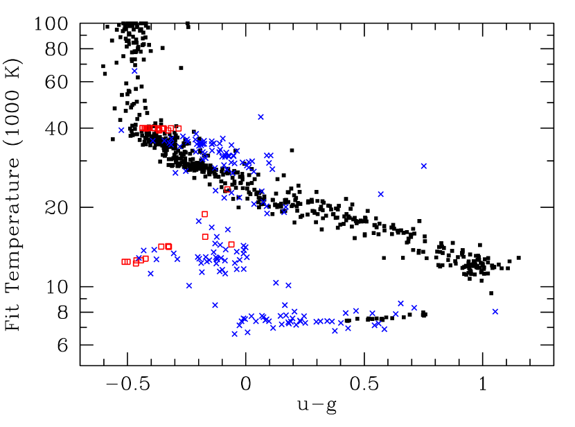
Figure 12: The locus of $u-g$ color versus autofit temperature for stars classified as hot subdwarfs. The color is corrected for interstellar extinction assuming that the star lies behind the Schlegel et al. (1998) prediction. Note that this is $u-g$ color, not $u-r$ as in Figures 7 and 8. We divide the single stars from those with companions by a cut of $g-r<-0.3-0.2(u-g)$ (see Fig. 4). The black dots show single stars fit to hydrogen atmospheres. These show a tight locus. The temperature scale is surely wrong, as hot subdwarfs commonly have mixed hydrogen-helium atmospheres that would bias the results, but the autofitting is recovering a general temperature trend. The red squares show single stars fit to a helium atmosphere. These temperatures have no correlation with colors, and the set at 40,000K is due to the limits of the fitting. Clearly, sdO atmospheres are not reliably matched by pure helium WD atmospheres. The blue crosses show the locus of color versus temperature for the binary stars. The spectroscopic fit obviously has enormous errors due to the change in line strengths for the composite spectra.

As noted above, the autofit temperatures and gravities are not correct in detail for the hot subdwarfs because these stars often show mixed element atmospheres, whereas we have only used single-element atmosphere models. However, it is likely that autofit does contain some information. Figure 12 shows the distribution of autofit temperatures and $u-g$ colors. Many of the points fall along a clean locus. Most of the outliers are also outliers in the $u-g$ versus $g-r$ color plane. This extra sequence is due to the presence of a main sequence companion that makes the $g-r$ color redder and also tends to dilute the deep SD lines (B. Green, private communication).

5.4 Testing autofit with duplicate spectra

Because we have more than one spectrum of some of the white dwarfs, we have the opportunity to test the stability of the autofit results. There are 775 duplicate spectra of white dwarfs in the catalog. For 617 of these, the primary spectrum have the autofit quality flag set, meaning that they are classified simply as DA or DB (possibly with colons) and that the autofit model used appropriate element in the atmosphere. In 20 of these cases, the secondary spectrum fails the autofit quality flag, and so we are left with 597 objects to compare. These objects have completely separate spectra, taken on different nights, often through different fibers on the spectrograph. The autofit analyses do share the same photometry. Our general sense, however, is that the photometry is very subdominant in the fitting and serves primarily to break ties between multiple minima in the spectral fitting.

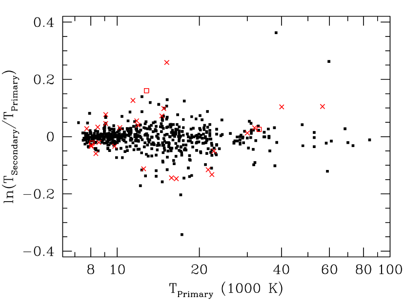
Figure 13: For the duplicate spectra, the ratio in autofit temperature between the two spectra (shown as natural log of the ratio) versus the temperature of the primary spectrum. Only stars for which the autofit was considered good in both observations are shown; this leaves 597 duplicate observations. Good means simply that the star was classified as a DA, DA:, DB, or DB: and that autofit used the appropriate element for the model fit. Stars with 3 observations are shown twice, once for each secondary observation. Objects whose deviation is less than $3-\sigma$ for the quoted formal errors are shown as black solid dots. The 26 cases where the residuals are between 3 and 5 $\sigma$ are shown as red crosses. The 3 cases where the residuals are more than 5 $\sigma$ are shown as red open squares. Note that most of the worst deviations are properly reflected in the errors.

Figure 13 shows the ratio in fitted temperatures as a function of temperature. In most cases, the agreement is close. We can also compute the formal error on the ratio. This shows that in most cases, the residuals are as expected from the autofit quoted errors. Only 29 systems have more than 3 $\sigma$ residuals, and only 3 more than 5 $\sigma$. Interestingly, the worst absolute residuals generally do not have high statistical significance, meaning that the formal errors are reporting the uncertainties. Separating Figure 13 into DA and DB stars doesn’t change the behavior.

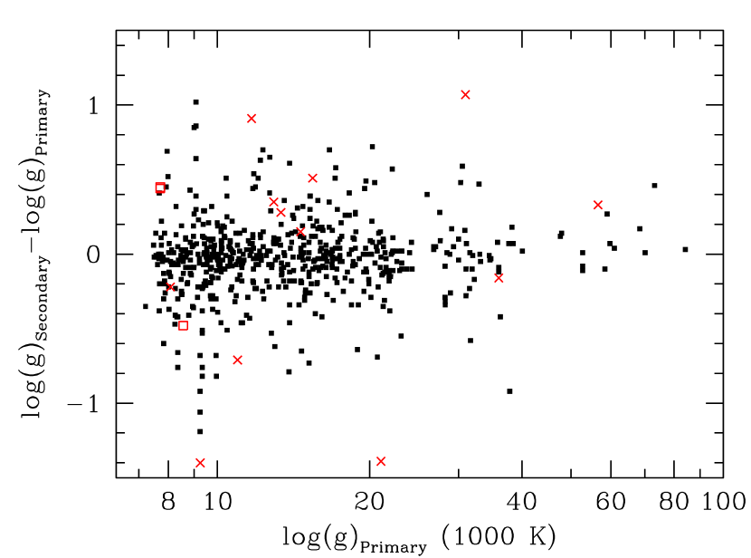
Figure 14: As Figure 13, but for surface gravity. The difference in $\log_{10}g$ is shown. There are 3 objects with residuals worse than 5 $\sigma$ and 12 between 3 and 5 $\sigma$. Again, although some of the absolute residuals can be large, these are typically reflected in the quoted errors.

Figure 14 is a similar plot, but now for the difference in the logarithm of the fitted surface gravity. There are 15 3 $\sigma$ outliers and 3 5 $\sigma$ outliers.

Finally, Figure 15 shows the residuals in $\log g$ versus the residuals in $T$, both normalized by the formal errors. If the errors were Gaussian, independent, and described by the formal errors, then this would be a normal Gaussian distribution in both axes. Aside from the handful of outliers, this is not far from the case. The central core appears to be about 20% broader than the unit normal, meaning that the formal errors are about 20% too small. There is a hint that brighter stars have slightly more scatter relative to their errors, say 40% rather than 20%, and all 5 of the 5 $\sigma$ outliers are brighter than $g=18$. We repeat the caveat, however, about the errors being badly underestimated near the model grid boundaries.

It is worth noting that the secondary observations were not visually inspected. The inspections of the primary observations were triggered by factors that could indicate data problems or suggest a classification other than DA or DB. If a data artifact was so bad as to prevent classification, then the star would be excluded from this comparison. However, aside from this, data problems will remain in both the primary and secondary observation, and only if the problems confused autofit into using the wrong element would the star not enter this comparison. Hence, we conclude that the formal errors in the autofit method are properly incorporating the uncertainties from data problems. This is in large part a statement that the formal errors on the SDSS spectra are reasonable, at least blueward of 7000Å. Of course, the results in this subsection on the stability of the autofit method only test the statistical errors and some observational systematics errors in the fitting. Systematic errors from the model atmospheres, from the autofit methodology, or from a generic bias in the SDSS dataset would not be revealed by comparing duplicate observations.

5.5 Comparison to the Literature

We next compare our fits to those in the literature. We find 71 fits of 46 stars in the literature that we can compare to ours (Bergeron et al., 1992, 1994; Marsh et al., 1997; Vennes et al., 1997; Finley et al., 1997; Homeier et al., 1998; Napiwotzki et al., 1999; Koester et al., 2001; Liebert et al., 2005). Figure 18 compares the surface gravities from the literature and autofit; the correlation implies that autofit is recovering the same signal as other analyses. Figures 16 and 17 show the residuals in the comparison as a function of temperature. Below 30,000 K, the comparison suggests no systematic offset, save for the fitting artifact in surface gravity for temperatures below 10,000 K. However, for temperatures above 30,000 K, there is a clear systematic trend for autofit to be higher in temperature and in surface gravity than the literature fits. The residuals are at least 10% in temperature above 50,000 K. We note that our modeling was already known to be wrong due to neglect of non-LTE physics and impure hydrogen atmospheres, but the literature fits are for the same assumptions and so should be comparable.

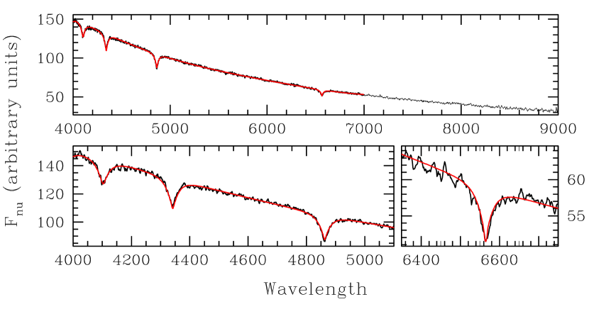
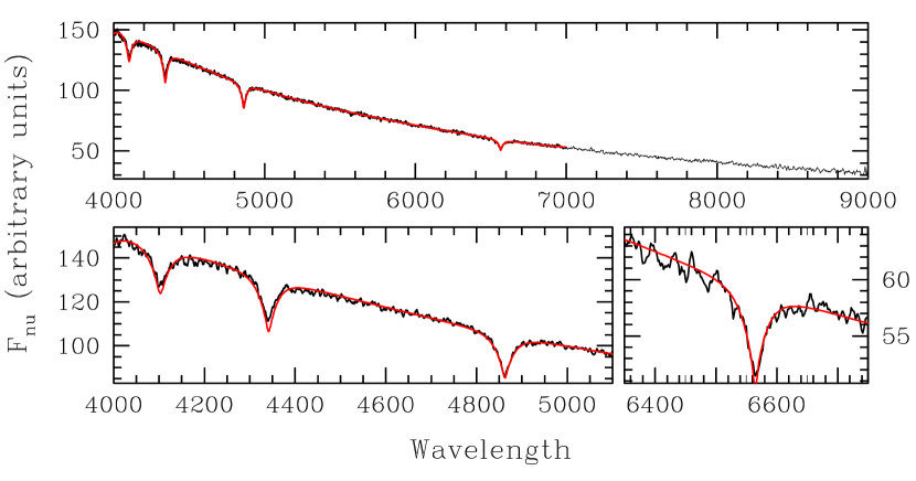
Figure 19: The spectrum and modeling for the hot DA SDSS J165851+341853, also known as WD1657+343 (Green et al., 1986; McCook & Sion, 1999), chosen to display the systematic shift between autofit and the literature for hot DA stars. The top two panels show the spectrum overplotted with the best autofit fit of $T=60,943$ K, $\log g=7.84$. The bottom two panels show the spectrum overplotted with $T=53,011$ K, $\log g=7.757$ (Finley et al., 1997). One sees that the H$\gamma$ and H$\delta$ lines are too deep and too broad in the lower temperature model. The higher temperature model is clearly the superior fit to the SDSS data given our modeling assumptions and there is no sign of any error in matching the continuum. Indeed, the problem seems to be a small residual error in the SDSS spectrophotometry.

We inspected our fits for these stars and found no sign of a systematic problem in the autofit method. For the SDSS data and the assumed models, the fits appear reasonable. Using the literature temperature and gravities produce model H$\gamma$ and H$\delta$ lines that are clearly deeper and slightly wider than the data. There is no sign that the continuum fitting is playing a role in the offset, and the autofit values do not change substantially if we exclude data blueward of 4000Å. An example of this is shown for SDSS J165851+341853 (aka WD1657+343) in Figure 19.

We then compared some of the spectra from Liebert et al. (2005) to the corresponding SDSS spectra. We found systematic offsets in the depths of the H$\gamma$ and H$\delta$ lines, about 2% relative to the continuum, with a width of about 50Å. We believe that this is due to small systematic errors in the SDSS spectrophotometry at the locations of the Balmer lines, where the SDSS algorithm masks the data when fitting the F subdwarf spectrophotometric stars. When we use the autofit program on the spectra from Liebert et al. (2005), we find temperatures and gravities that agree well with the literature. The temperature comparison is shown in Figure 20; the gravities do not shift and continue to agree.

These spectrophotometric residuals are small, but since they are similar in breadth to the lines of a hot DA, they do affect the temperatures. The bias is quite small at lower temperatures when the Balmer lines are strong, but becomes noticeable with the weaker lines of the hottest DAs. Of course, this effect is negligible for most non-WD applications; for narrow lines, most SDSS spectra lack the signal-to-noise ratio to even detect a 2% residual.

We are investigating methods to address this problem in future catalogs. At this point, users of our catalog should be cautious about the exact temperature scale of the hot DA stars, even beyond the usual caveats of non-LTE and multi-element atmosphere modeling.

5.6 Completeness

White dwarfs enter the SDSS spectroscopic sample through several different targeting programs, all of which have different color, magnitude, and photometric quality cuts as well as different priorities and sparse samplings. As such, we have not yet attempted to reconstruct in full detail the completeness of the targeting. However, we have done some work on this topic, which we report in this section. Note that this section is only about what objects had a spectrum taken of them, not whether we have properly identified the spectrum as that of a white dwarf.

We will assess the completeness by selecting from the DR4 imaging catalogs all blue point sources with good photometry in all 5 bands (good being defined by the “clean sample” set of flag checks defined in the DR4 on-line documentation). After removing those objects that are not covered by a spectroscopic plate, we then find the fraction of these targets of which a spectrum was taken. This fraction, as a function of magnitude, color, galactic position, etc, is the completeness map.

We focus here on very blue point sources with colors typical of single white dwarfs. We restrict ourselves to $u-g<0.7$, $g-r<-0.1$, and $r-i<-0.1$, dereddened. This is where white dwarfs hotter than about 12,000 K reside, but it is also the region where objects were excluded from the optical quasar selection (Richards et al., 2002), save for in the earliest SDSS data. Objects with blue $u-g$ colors but redder colors in either $g-r$ or $r-i$ are targeted as quasars (down to $i<19.1$) with high completeness. Hence, the white dwarfs in this color region enter the sample by one of the stars, serendipity, or standards targeting packages.

An important thing to note is that all of the stars, serendipity, and standards classes in the normal SDSS survey require that the target not be blended on the sky with any other object. By this, we do not mean that the object must be successfully deblended (although most deblends are successful), but that it could not have been blended in the first place, meaning that the reference isophots cannot touch. The stars must also not be near the edge of a chip. These are stringent cuts, intended to boost the purity of the sample. The exact flags are EDGE, CHILD, and BLENDED; none can be set.

We find that the fraction of sources with good photometry that pass the not-blended cut is only about 60%. This fraction is mildly dependent on galactic latitude: 55% at $30^{\circ}$, 60% at $40^{\circ}$, and 63% at $70^{\circ}$. But it is strongly dependent on magnitude: 40% at $g=15$, 55% at $g=17$, 63% at $18<g<19.5$. The reason for this is brighter stars reach the isophotal threshold at larger radius and hence have more opportunity to be blended with fainter objects. Closer to the galactic plane, the latitude dependence does steepen as one would expect.

Focusing now on the non-blended stars, the completeness is still imperfect because of the selection cuts and the sparse sampling. The key set here is the “Hot_Standard” class, which requires $u-g<0$, $g-r<0$, and $g<19$, dereddened (Kleinman et al., 2004). This class was observed with high priority as a tiled class (Blanton et al., 2003a), and the selection will include most of the brightest hottest stars. However, the selection also required a fairly stringent photometric quality flag, more stringent than the survey currently recommends. As such, the spectroscopic completeness for this color-magnitude box is 77% of the non-blended stars. For fainter stars in the range $19<g<19.5$, this completeness drops to 50%, as these stars enter from other stars and serendipity selections. We find no measurable dependence on $u-g$ in either of these computations.

For stars at $0<u-g<0.7$, $g-r<-0.2$, $r-i<-0.1$, and $g<19.5$, dereddened, we find that the completeness is about 50% of the non-blended stars, with no measurable dependence on $u-g$. For $-0.2<g-r<-0.1$, the completeness is mildly lower, about 40%.

The actual completenesses will be somewhat lower because our parent sample required good photometry in all bands. It is not correct to compute this completeness correction by asking what fraction of bad photometric objects got spectra, because many of the objects with bad photometry are not hot stars but were simply scattered into the color box as outliers. Of course, bad things sometimes happen to good stars, but one has to compute this fraction based on simulations of fake stars through the photometric pipeline. This failure branch is likely of order 5%, but we have not quantified it in this paper.

We also have not studied the completeness for $g>19.5$, for $u-g>0.7$, or for other red portions of color space, as this is not where the bulk of our catalog lies.

The SDSS does not target bright stars, as they saturate the spectrograph and harm the extraction of traces from other fibers. The stars and serendipity packages all require the object to have fiber magnitudes fainter than 15 in $g$, $r$, and $i$. The PSF magnitudes are about 0.3 magnitudes brighter than the fiber magnitudes. Completeness brighter than $g<14.8$ will be poor, but we have not assessed this further.

Returning to the blended stars, the completeness within the SDSS is below 10%. Blended stars can enter through the quasar or ROSAT target algorithms. Both have important color selections, and it is clear that the blended stars in this WD catalog are typically much redder than the unblended stars (closer to quasar colors). With the completeness so low and possessing an uncharacterized color bias, we recommend that blended stars be avoided for statistical analyses.

We have marked the stars in the catalog as to whether they are unblended or not. Some of these blended stars have entered through the southern special target selection, in which the quasar selection was performed without the usual exclusion of the WD region (Adelman-McCarthy et al., 2006). A few may have entered in the unusual case where the targeting was done on different imaging or earlier reductions than the “best” match in DR4 (which is what we use to report the blending status).

We note that binary stars typically do not get reported as blended. Two point sources need to be a few arcseconds apart to be recognized as two peaks by the deblender. Many binary systems are unresolved in the SDSS and simply appear as objects with unusual colors and spectra. Intermediate systems, e.g., those 0.3-$3^{\prime\prime}$ apart, will be marked as single objects but detected as extended. These will then be rejected by all stellar targeting classes, but picked up by galaxy targeting down to $r=17.77$ (Strauss et al., 2002).

In short, we expect that the completeness on hot single stars in the range $14.8<g<19.5$ is essentially the product of a magnitude-dependent factor of 40-60% because of the not-blended criteria and another factor of 40-77% depending on color and magnitude. Incompleteness of the parent imaging catalog or of our spectroscopic classification are additional factors, expected to be small for common classes of white dwarfs.

6 Low-mass White Dwarf Candidates

Liebert et al. (2004) presented two DA stars (and 6 other candidates) with unusually low surface gravities and hence low masses. SDSS J123410.37-022802.9 in particular was found to be at 17,500 K and $\log g=6.38\pm 0.05$, implying a mass of $0.19\rm M_{\odot}$. Other examples of white dwarfs of similar mass are MSP J1012+5307 (Van Kerkwijk et al., 1996), HD188112 (Heber et al., 2003), and the companion to PSF J0751+1807 (Nice et al., 2005). White dwarfs with masses this small are thought to be composed of helium cores rather than the canonical carbon-oxygen cores. Such stars can be formed when a companion strips the outer envelope from a helium-core post-main-sequence star. The existence of two of these rare stars around pulsars (Van Kerkwijk et al., 1996; Nice et al., 2005) suggests that the involvement of a neutron star may be an important pathway for the formation of the low-mass white dwarf (Liebert et al., 2004).

Here we discuss 13 low-mass candidates from the DR4 catalog, 4 of which overlap the list in Liebert et al. (2004). These objects are selected to have temperatures less than 30,000K, surface gravities more than 2 $\sigma$ below 7.2, and $g<20$. We summarize the candidates in Table A Catalog of Spectroscopically Confirmed White Dwarfs from the Sloan Digital Sky Survey Data Release 4.

Most of the candidates are similar to SDSS J123410.37-022802.9 in that they have temperatures between 15,000 and 20,000 K and gravities between 6.2 and 7.0. However, 3 of the candidates are significantly lower temperature, suggesting even smaller masses.

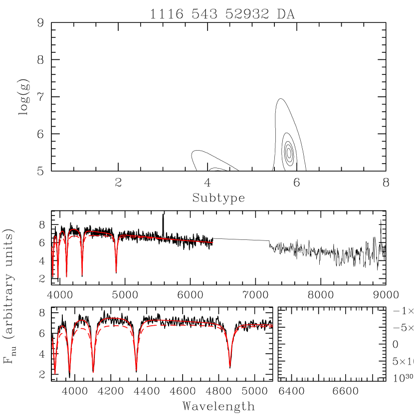
Figure 21: The spectrum and autofit model for low-mass candidate SDSS J204949.78+000547.3. The likelihood contours show evidence for multiple minima. The best fit to the spectroscopy is at $T=8660$ K and $\log g=5.48$, but the photometry supports a higher temperature and lower gravity, closer to the secondary minimum.

SDSS J204949.78+000547.3 is our lowest gravity candidate. The best fit to the spectroscopy is 8660 K with $\log g=5.48\pm 0.10$. However, as Figure 21 shows, the likelihood surface has a second minimum at roughly 11,500 K and even lower gravity. The primary photometry of this has a corrupted $g$ band, which was excluded from the fit. However, this star, being on the equator in the south Galactic cap, has been imaged eight times during the SDSS. The averaged photometry (excluding the one bad $g$ observation) is $u=20.29\pm 0.02$, $g=19.20\pm 0.01$, $r=19.36\pm 0.01$, $i=19.51\pm 0.01$, and $z=19.60\pm 0.04$. The field is highly reddened, with a $g$-band extinction of 0.39 mag. If we apply the full dereddening, then the colors become $u-g=-0.95$, $g-r=-0.27$, $r-i=-0.22$, and $i-z=-0.15$. These colors do not match the 8660 K, $\log g=5.48$ solution, and instead prefer the hotter, lower gravity solution. In short, the colors are more similar to a horizontal branch star, but the spectral lines are clearly broader than that. SDSS J204949.78+000547.3 remains unexplained.

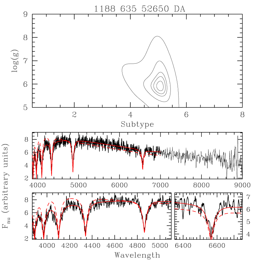
Figure 22: The spectrum and autofit model for low-mass candidate SDSS J084910.13+044528.7. The best fit to the spectrum is $T=9962$ K and $\log g=5.93$; the photometry is consistent with these values.

SDSS J084910.13+044528.7 (Fig. 22) is a less extreme but more secure candidate. The best fit is $9960\pm 170$ K, $\log g=5.93\pm 0.15$. The dereddened colors of $u-g=0.88\pm 0.05$, $g-r=-0.17\pm 0.03$, $r-i=-0.18\pm 0.03$, $i-z=-0.29\pm 0.08$ are a excellent match to the predicted colors of this fit. The cooler temperature and lower gravity than SDSS J123410.37-022802.9 favor an even lower mass. Of course, at 10,000 K, one is beginning to reach the point where autofit gravities tend to be overestimated. It is unknown whether the bias at higher gravities extends to lower gravities, but if it does, then the true gravity might be somewhat lower than 5.93. In any case, the spectrum of SDSS J084910.13+044528.7 clearly has broader lines than a main sequence A star or blue horizontal branch star.

Low temperature, low-mass stars such as these are incomplete in our catalog simply because of the initial color cut, which was intended to exclude main sequence and blue horizontal branch stars. However, stars of these colors do receive a healthy allocation of spectroscopic fibers in the SDSS as part of the blue horizontal branch target selection. We plan a more focused search for these stars in the future.

Two other candidates have multiple epochs of photometry. SDSS J225242.25-005626.6 has been observed 9 times with photometry $u=18.81\pm 0.01$, $g=18.61\pm 0.01$, $r=18.85\pm 0.01$, $i=19.07\pm 0.01$, and $z=19.27\pm 0.03$. SDSS J002228.45+003115.5 has been observed 10 times with photometry $u=19.51\pm 0.03$, $g=19.34\pm 0.02$, $r=19.63\pm 0.02$, $i=19.86\pm 0.01$, and $z=20.11\pm 0.05$. Using this photometry in the fitting doesn’t change the best fits. We have included this photometry in Table A Catalog of Spectroscopically Confirmed White Dwarfs from the Sloan Digital Sky Survey Data Release 4 but not in the primary catalogs.

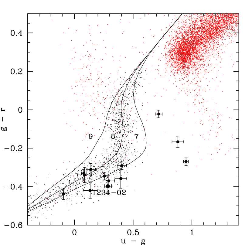
Figure 23: The $g-r$ and $u-g$ colors (dereddened) of the 13 low-mass candidates, overlaid on a background of DAs (small black points) as well as model predictions for DA colors at varying temperature at $\log g=7$, 8, and 9. Small red points show a very sparse sampling of main sequence stars, horizontal branch stars, and quasars from Harris et al. (2001). See Figure 1 for the realistic distribution. The confirmed object SDSS 1234–02 is labeled and has a somewhat larger symbol. Most of the candidates lie in the expected region of color space, but three have more normal colors such that one would have to appeal to some mild photometry errors. The low temperature cases lie well off the DA locus but still somewhat blueward of the horizontal branch.

Figure 23 shows the $u-g$ vs. $g-r$ colors of these stars, overlaid with the constant surface gravity model tracks. One sees that most of the candidates do lie redward of the $\log g=7$ track in $u-g$, although in three cases, one would need to invoke some mild photometric error. Figure 24 shows the temperature and surface gravity distribution overlaid with constant-mass predictions from Althaus et al. (2001). These tracks suggest that these white dwarfs are below $0.3\rm M_{\odot}$, with 7 at or below $0.2\rm M_{\odot}$. The two stars discussed above, SDSS J204949.78+000547.3 and SDSS J084910.13+044528.7, may be the lowest mass white dwarfs yet found. Given the recent discovery of a second massive pulsar around a helium-core white dwarf (Nice et al., 2005), these low-mass stars should be investigated for signs of a neutron star.

In round numbers, models for these stars typically predict absolute magnitudes of $M_{g}\sim 8.5$. This means that SDSS can recover the stars at distances between 200 pc and 2 kpc. At the high Galactic latitudes of this catalog, we are probing out up to several disk scale lengths. A detailed analysis of the space density of these stars will have to wait for a full completeness analysis, but clearly the stars are rare, with only 13 observed (times a yet-to-be-determined completeness factor) over a survey volume of 4 kpc³.

7 The Hot Subdwarf Sequences

The hot subdwarfs consist of two groups: 1) a sequence of generally helium-rich sdO stars that have blackbody-like colors and largely coincide with the DO-DB sequence, and 2) a sequence of hydrogen-rich sdB stars. The latter are also called extended horizontal branch (EHB) stars when they are found in globular and Galactic star clusters.

The $u-g$ and $g-r$ colors of our hot subdwarfs are shown in the bottom, right panel of Figure 4. Isolated stars run along the bottom (bluer in $g-r$), with the sdO stars at the bluest tip. The $u-g$ vs. $g-r$ color distribution shows two interesting features. First, there is a second locus in color that falls redward in $g-r$ of the primary sequence. These are subdwarfs with cool, nondegenerate binary companions. These main-sequence stars redden the longer wavelength colors. Unlike white dwarfs, which are so faint as to be overwhelmed by anything but a M dwarf, the subdwarfs can be blended with F or G main-sequence stars and still show a very blue $u-g$ and $g-r$ color. As shown in Figure 12, the companion star does corrupt the spectral fit.

Second, the single star locus stretches continuously from the bluer ($u-g<0$) end through to the edge of our selection at $u-g\approx 1$ where the locus joins that of the more common blue horizontal branch (BHB) and blue straggler stars (BSS) near 10,000 K. Traditionally, stars classified as sdB have been hotter than 20,000 K; for example, the analyses of Moehler et al. (1990) and Saffer et al. (1994) only included stars with derived $T_{\rm eff}\geq 23,000$ K. Such stars would likely be at $u-g<0$. However, Figure 4 clearly shows that the hydrogen-rich sequence extends redward and is continuous down to the BHB and BSS region, such that the horizontal branch is populated from 10,000 K to near 40,000 K (Greenstein & Sargent, 1974).

There are two important complications in interpreting the distribution of stars along this locus. First, the SDSS target selection is not uniform across this region. The “Hot_Standard” class gives high priority to targets with $u-g<0$ and $g<19$. Redder stars are still targeted, largely through the blue-horizontal-branch selection (Yanny et al., 2000; Newberg et al., 2002), but the completeness is not as high. Second, the depth of the SDSS sample is such that different Galactic populations are being probed by the different types of stars. Notably, the BHB stars are a halo population while the EHB sample is primarily a disk population. We are postponing analysis of this locus to future work.

8 Conclusions

We have identified 9316 spectroscopically confirmed white dwarfs and 928 hot subdwarfs from the 800,000 spectra of the SDSS Data Release 4. Rolling together all secondary classifications, the sample includes 8000 DA, 713 DB, 289 DC, 41 DO/PG1159, 104 DQ, and 133 DZ stars. There are of course many different mixed and subclassifications. More than 6000 of these WDs are new, so this catalog roughly doubles the number of spectroscopically confirmed white dwarfs.

We have fit model atmospheres to the DA and DB stars using our autofit method. We find the expected strong peak in surface gravity, along with interesting outliers, such as the low-mass candidates discussed in § 6. The fitting results are validated for internal consistency using repeat observations and by correlations with the photometry. There is a systematic bias toward higher gravities at lower temperatures of which users should beware. This appears to be an artifact of the model atmospheres. There is also a bias toward over-estimating the temperature of DA stars above 30,000 K. This is caused a subtle systematic error in the SDSS spectrophotometry causing the broad Balmer lines in the blue to be slightly filled in.

Among our fitted stars, we continue to find a rare population of low surface-gravity candidates that are very likely helium-core, low-mass DA white dwarfs, building on the sample of Liebert et al. (2004). Two of these candidates may be the lowest mass DA stars yet found, although this awaits confirmation. These stars are very similar to the two companions of massive pulsars (Van Kerkwijk et al., 1996; Nice et al., 2005), opening the hypothesis of a generic evolutionary role for neutron star companions in the formation of these white dwarfs.

We cannot claim that this catalog is complete, particularly for difficult cases such as DC stars, low-temperature DA stars, binary systems, and DH stars. For mundane warm to hot isolated DA, DB, and DO stars (above $\sim\!8,000~{}K$ for DA stars), we believe that the catalog should be reasonably complete (95% or more) within the SDSS spectroscopic catalog and down to spectral signal-to-noise ratios where one can expect to classify the stars.

In addition to searching for unusual classes of white dwarfs, large catalogs open the possibility of large-number statistical studies of the distribution of white dwarf properties as well as their Galactic structure. Although the SDSS spectroscopic target selection is not complete for these stars, the incompletenesses can be modeled. We have discussed the key aspects of this modeling in § 5.6.

The SDSS DR4 represents roughly half of the final spectroscopic sample for the original SDSS survey. In addition, the new Sloan Extension for Galactic Understanding and Exploration (SEGUE) is conducting an extensive study at lower Galactic latitudes with both imaging and spectroscopy. Although white dwarfs are rare within the SDSS catalogs, the available numbers are sufficient to open a key new opportunity to study this diverse category of stars.

We thank Detlev Koester for providing grids of his recent model atmospheres. We thank Betsy Green and Gary Schmidt for useful discussions. We thank David Johnston and Ryan Scranton for use of their stacked catalogs from the SDSS equatorial region and Jay Holberg for help matching to the McCook & Sion (1999) catalog. DJE was supported by NSF AST-0098577 and AST-0407200 and by an Alfred P. Sloan Research Fellowship. JL was supported by NSF AST-0307321.

Funding for the Sloan Digital Sky Survey (SDSS) has been provided by the Alfred P. Sloan Foundation, the Participating Institutions, the National Aeronautics and Space Administration, the National Science Foundation, the U.S. Department of Energy, the Japanese Monbukagakusho, and the Max Planck Society. The SDSS Web site is http://www.sdss.org/.

The SDSS is managed by the Astrophysical Research Consortium (ARC) for the Participating Institutions. The Participating Institutions are The University of Chicago, Fermilab, the Institute for Advanced Study, the Japan Participation Group, The Johns Hopkins University, the Korean Scientist Group, Los Alamos National Laboratory, the Max-Planck-Institute for Astronomy (MPIA), the Max-Planck-Institute for Astrophysics (MPA), New Mexico State University, University of Pittsburgh, University of Portsmouth, Princeton University, the United States Naval Observatory, and the University of Washington.

Figure 2: The autofit temperature and gravities for all of the stars in our parent list that were fit to hydrogen atmospheres and that were visually classified in the DR1 WD catalog (Kleinman et al., 2004). The upper panel shows those classified as white dwarfs; the lower panel shows those classified as non-WD. In each panel, lines divide the plot into three regions marking the autofit first-pass classification: upper-left for DA white dwarfs, lower-left for subdwarfs, right for unknown. The crosses show objects selected for visual inspection. The squares show objects for which the autofit result would have been accepted were we not applying the visual classifications from Kleinman et al. (2004). The figures show that nearly all of the automatically classified white dwarfs (squares in the upper left) are white dwarfs: there are only 5 squares in the upper left of the bottom panel. Moreover, nearly all of these stars were visually classified as DAs: in the top panel, we mark DAs with solid squares and other WDs with open squares. The upper left region of the top panel contains about 1700 autoclassified stars, all but 2 of which are DAs. Non-DA white dwarfs may fall in that region, but they were selected for inspection. Squares in the other regions in the top panel mark white dwarfs that were not recovered, having been accepted as other types. These are also rare.

Figure 3: The autofit temperature and gravities for all of the stars in our parent list that were fit to helium atmospheres and that were visually classified in the DR1 WD catalog (Kleinman et al., 2004). The lines show the autofit first-pass classifications: upper-left for DB white dwarfs, bottom for subdwarfs, upper-right for unknown. The solid squares are visually classified DBs that were selected for inspection (we selected the whole first-pass DB region for inspection so as to improve the catalog for the rarer DBs). The open squares are visually classified DBs that were not selected for inspection and hence would have been missed. The crosses are other objects selected for inspection; the triangles are other objects rejected by autofit. The other objects are often other classes of white dwarfs or cataclysmic variables, since low-temperature helium atmospheres have featureless continua that become the best-fit model in our limited fitting space.

=7inugr_mosaic.eps

Figure 4: The $u-g$ vs $g-r$ colors of stars in sets according to their classification. The photometry has been corrected for interstellar extinction (Schlegel et al., 1998), assuming that the stars lie behind the full dust screen. Stars that are closer than that will be overcorrected and therefore be bluer on this plot than they intrinsically are. Stars that are given an uncertain classification are included in this plot. The solid black lines shows the color cut applied to the selection of the sample. The dashed line at $g-r=0.2$ is to remind the reader that redward of this cut, the object is also required to lie off of the main-sequence locus in $g-r$ and $r-i$. (upper left)) DA classified stars. An approximate fit to this locus is reproduced on the other panels so that the reader may compare. (upper right) DB, DO, and DC stars. (middle left) DZ stars. (middle right) DQ stars. (lower left) All white dwarfs that are classified as having a companion. As expected these stars lie redward than the single star locus, particularly in $g-r$. lower right) Hot subdwarfs. The locus tracking below the DA line is the single star locus; hot subdwarfs with companions form the sequence that falls closer to the helium atmosphere line. The single star locus extends to rather red $u-g$ colors; however, our division between sdB and BHB stars is probably too generous. It is also inconsistent; there are many stars at $u-g\approx 1$ that were rejected as A or BHB stars.

Figure 7: The locus of $u-r$ color versus autofit temperature for stars classified as DA or DA: and fit to a hydrogen atmosphere. The color is corrected for interstellar extinction assuming that the star lies behind the Schlegel et al. (1998) prediction. The correlation between color and temperature is generally excellent, with slightly more scatter around the instability strip at 11000 K. While the photometry is used in the fit, it does not dominate the result; we regard the agreement as demonstration that the spectroscopic fits are well-correlated with temperature. Note that some of the scatter is simply due to variations in surface gravity.

Figure 8: The locus of $u-r$ color versus autofit temperature for stars classified as DB or DB: and fit to a helium atmosphere. The color is corrected for interstellar extinction assuming that the star lies behind the Schlegel et al. (1998) prediction. The correlation between color and temperature is encouraging. The solid dots are spectra with $S/N>10$ per spectroscopic pixel; crosses are those with lower signal-to-noise ratio. One sees that there are high S/N cases across the full temperature range, including stars above 25,000K.

Figure 9: The locus of autofit surface gravity versus autofit temperature for stars classified as DA or DA: and fit to a hydrogen atmosphere. Only stars with $S/N>10$ per spectroscopic pixel in the $g$-band are plotted. The well-known peak at $\log g=7.9$ is clear, but the scatter around this relation is largely real. One also sees the systematic bias toward higher gravities at lower temperatures. As discussed in the text, this is likely due to systematic errors in the model atmospheres at low temperatures. Values very close to the boundaries of the model grid (notably at $\log g=9$ or $T=10^{5}$ K tend to pull artificially to the boundary and have their error underestimated.

Figure 10: As Figure 9, but for stars with $S/N<10$ per pixel. The scatter is clearly larger, but the distribution is otherwise unchanged.

Figure 11: The locus of autofit surface gravity versus autofit temperature for stars classified as DB or DB: and fit to a helium atmosphere. Stars with $S/N>10$ per spectroscopic pixel in the $g$-band are plotted with solid points; stars with $S/N<10$ are plotted as crosses. As with the DA stars, the peak in $\log g$ is recovered at higher temperatures, but lower temperatures have a systematic bias toward higher surface gravities.

Figure 15: For the duplicate observations, the residuals in surface gravity versus the residuals in temperature, both normalized by the formal errors from autofit. We use the natural logarithm of the ratio of the two temperatures for the temperature residual, and the difference of $\log_{10}g$ for the surface gravity residual. In both cases, the error $\sigma$ is that of the residual from the combination of the formal errors. All 597 duplicate observations in which the autofit was considered good are shown. Aside from a few outliers, most observations lie in a tight locus that is close to a normal Gaussian. In detail, the formal errors appear to be underestimated by about 20%.

Figure 16: The comparison of autofit temperature to fits from the literature. We see clearly that autofit temperatures become systematically higher than the literature values for white dwarfs above 30,000 K. The literature values have been separated into three groups to show the consistency in values between various groups. Open circles are from Bergeron et al. (1992), Bergeron et al. (1994), and Liebert et al. (2005).. Filled circles are from Finley et al. (1997), Homeier et al. (1998), and Koester et al. (2001). Stars are from Marsh et al. (1997), Vennes et al. (1997), Napiwotzki et al. (1999).

Figure 17: The comparison of autofit surface gravities to fits from the literature, as a function of temperature. At low temperatures, autofit gravities are systematically high; this is due to the modeling inconsistencies and grid artifacts discussed in § 5.2. We also see a trend at high temperatures for autofit to be high. This is related to the trend seem in the comparison of temperatures, as there is a degeneracy in which displacements to higher temperatures and higher gravities have compensating effects in the spectrum. The symbols are the same as in Figure 16.

Figure 18: The comparison of autofit surface gravities to fits from the literature. A high level of correlation is seen; in a broad sense, autofit is recovering the same trends as other analyses. The symbols are the same as in Figure 16.

Figure 20: The comparison of autofit temperatures to fits from Liebert et al. (2005) for two sets of spectra on a group of stars. The crosses show the fits to the SDSS spectra; the solid points show the fits to the Liebert et al. (2005) spectra. This demonstrates that autofit gives similar temperatures to the fits of Liebert et al. (2005), but that the two sets of spectra are systematically different. We believe that this is due to spectrophotometry residuals in the SDSS at the H$\gamma$ and H$\delta$ lines.

Figure 24: The fitted surface gravity and temperatures of the 13 low-mass candidates, overlaid on tracks of constant mass from Althaus et al. (2001). Also shown are the tracks of the zero-age main sequence (ZAMS) and horizontal branches (BHB and EHB). The confirmed objects MSP J1012+5307 (Van Kerkwijk et al., 1996) HD188112 (Heber et al., 2003), and SDSS 1234–02 (Liebert et al., 2004) are labeled, the first as PSR because it is around a known pulsar. The low-temperature candidates may be the lowest mass white dwarfs yet found.

Table 1:

White Dwarf Dominant Classifications
Classification^a Number DA 8000 DB 713 DC 289 DH 9 DO 31 DQ 104 DZ 133 PG1159 10 WD 27 NOTES.—^a This classification refers to the dominant classification, given by the first two letters of the full classification. WD means that the type of the WD was not clear.

Table 2:

Class	Number	Class	Number
DA	2080	DB+M:	5
DA:	163	DB O:	1
DA auto	4919	DB: or HeSDB	3
DAB	7	DB:+QSO:	1
DA B:	2	DBZ	8
DAB:	1	DB Z:	1
DABH	1	DBZ:	1
DA BH:	1	DBZA	3
DA CV:	4	DBZ A:	2
DA+dC	1	DC	142
DAE	1	DC:	131
DAH	46	DCA:	1
DA H:	10	DC:+M	5
DAH+DA:	1	DC+M	8
DA H:+M:	1	DC+M:	2
DAH+M:	1	DH	5
DAHpec	2	DH:	3
DA+K:	1	DH+DA	1
DA:+M	30	DO	19
DA:+M:	5	DO:	9
DA+M	611	DO+M	3
DA+M:	81	DQ	45
DAO	13	DQ:	26
DAOB	2	DQABhot	1
DApec	3	DQAhot	3
DApec:	2	DQHhot	1
DA Q:	1	DQhot	18
DA+QSO:	1	DQhot:	2
DA:+sdK:	1	DQhot H:	2
DA+sdK	1	DQ:+M:	1
DAZ	4	DQpec	5
DAZ:	3	DZ	95
DB	508	DZ:	17
DB:	54	DZA	13
DBA	56	DZ A:	1
DB A:	28	DZA+M	1
DBA:	12	DZB	1
DBA:+M	1	DZBA	2
DBA+M	1	DZ:+M	1
DBApec:	1	DZ+M	2
DBAZ	6	PG1159	10
DB balmerE	1	WD	1
DBH	3	WD:+M	22
DB:+M	2	WD+M	2
DB+M	15	WD+M:	2

Table 3:

Classification	Number
HeSDB	5
HeSDB:	11
SD:	8
SD auto	391
SDB	195
SDB:	31
SDB+G	4
SDB+M	3
SDB+M:	1
SDB+MS:	7
SD:+M	1
SDO	218
SDO:	52
SDO+G:	1

Table 4:

Column	Description
1	Classification
2	McCook & Sion (1999) WD Catalog Identification Label (as of August 2005)
3	Provenance of the SDSS classificationa
4	Primary spectrum, $=0$ if a duplicate spectrum, $=1$ otherwise
5	SDSS IAU-style nameb
6	Right Ascension (J2000)c
7	Declination (J2000)c
8	Proper Motion (arcsec/century)
9	Proper Motion position angle (degrees), $=0$ for north, $=90$ for east
10–11	$\Delta$RA, $\Delta$Dec Proper Motion (arcsec/century)
12	Time of SDSS imaging observation (MJD)c
13	SDSS Run number
14	SDSS Rerun number
15	SDSS Camera Column
16	SDSS Field number
17	SDSS ID numberd
18–22	$u$, $g$, $r$, $i$, $z$ magnitudes (PSF, as observed)
23–27	$u$, $g$, $r$, $i$, $z$ magnitude errors
28–32	$u$, $g$, $r$, $i$, $z$ photometry flag summary ($=1$ for bad, $=0$ for good)
33	Extinction in the $g$ bande
34	Plate number
35	Fiber number
36	MJD number for spectroscopic observation
37	$S/N$ of spectrum in the $g$ band, per spectroscopic pixel
38	Deblended? $=1$ if the object was isolated, $=0$ if it was deblended.f
39	PrimTarget flag (decimal)g
40	PrimTarget flag (hex)g
41	SecTarget flag (decimal)g
42	SecTarget flag (hex)g
43	Autofit quality flag. $=1$ if good. If zero, do not use the autofit numbers for anything but diagnostic searching
44	Autofit atmosphere element ($=1$ for hydrogen, $=2$ for helium)
45	Autofit Temperature (Kelvin)
46	Autofit Temperature Error (Kelvin)
47	Autofit $\log g$ (dex)
48	Autofit $\log g$ Error
49	Autofit $\chi^{2}$ per degree of freedom

NOTES.—^a This is merely to track the provenance of our spectral classification; it does not indicate discovery nor literature classifications, which could be tracked through the McCook & Sion (1999) catalog. Kle04: Kleinman et al. (2004) Sil05: Silvestri et al. (2005) DR4: This paper. ^b This is the name from the SDSS DR4. Because of tiny astrometry shifts, it is possible that this name may differ from the name in previous SDSS releases. This breaks the IAU convention that published names never change. We strongly recommend that associations be performed on the astrometric coordinates rather than on the name. ^c The epoch of the coordinates is given by the time of the SDSS imaging observation in column 12. ^d ID number within the field, not the objID in the SDSS CAS. ^e The canonical SDSS extinction curve in $u$, $g$, $r$, $i$, and $z$ is 1.36, 1.00, 0.73, 0.55, and 0.39 times $A_{g}$. ^f Most of the relevant target selection catagories require that the object be sufficiently isolated on the sky that it was not blended with any other object. Blended stars have much lower completeness; see § 5.6. ^g These bit fields record the decisions from the various spectroscopic targeting algorithms. See Stoughton et al. (2002) and Adelman-McCarthy et al. (2006) or the on-line documentation for details. The southern survey bit (0x80000000) has been suppressed in the secTarget flag for brevity but retained in the primTarget flag (Adelman-McCarthy et al., 2006).

Table 5:

Name	Plate	MJD	Fiber	RA (J2000)	Decl (J2000)	Class
SDSS J020848.28+121332.4	0428	51883	246	32.20118	12.22568	DA
SDSS J144738.39+034930.4	0587	52026	118	221.90997	3.82511	DA
SDSS J102448.85–002312.3	0272	51941	180	156.20354	–0.38675	DA:
SDSS J124337.50+671252.1	0494	51915	033	190.90623	67.21448	DA:
SDSS J170919.90+612016.8	0351	51780	112	257.33293	61.33799	DA:
SDSS J102414.85+655551.6	0489	51930	338	156.06186	65.93099	DA6
SDSS J080755.99+485419.3	0440	51885	275	121.98330	48.90537	DA7
SDSS J104912.65–000854.8	0275	51910	110	162.30270	–0.14855	DA7
SDSS J115052.32+683116.1	0492	51955	523	177.71800	68.52113	DA7
SDSS J171713.11+574634.6	0355	51788	548	259.30463	57.77628	DA7
SDSS J105628.49+652313.5	0490	51929	205	164.11870	65.38707	DAH
SDSS J010352.23–100230.2	0659	52199	318	15.96764	–10.04172	DA:H:
SDSS J001733.59+004030.4	0389	51795	614	4.38997	0.67512	DAM
SDSS J032428.78–004613.8	0414	51901	263	51.11991	–0.77050	DAM
SDSS J081410.59+452315.7	0439	51877	583	123.54414	45.38770	DAM
SDSS J172043.87+560109.3	0367	51997	464	260.18281	56.01925	DAM
SDSS J155340.36+011335.3	0343	51692	367	238.41816	1.22647	DB
SDSS J160437.77+005206.7	0344	51693	523	241.15736	0.86853	DB
SDSS J091436.46+014514.5	0473	51929	319	138.65192	1.75403	DB:
SDSS J154938.64–001318.2	0342	51691	104	237.41101	–0.22173	DB:
SDSS J173327.35+585439.8	0366	52017	582	263.36394	58.91106	DB_UNC
SDSS J000116.53+000205.4	0387	51791	177	0.31887	0.03483	DC
SDSS J000918.12–002141.5	0388	51793	145	2.32550	–0.36152	DC
SDSS J005253.74+135618.2	0420	51871	207	13.22390	13.93839	DC
SDSS J012048.78–090740.9	0661	52163	393	20.20323	–9.12802	DC
SDSS J012723.62–004630.0	0399	51817	099	21.84843	–0.77500	DC
SDSS J025457.18–072641.8	0457	51901	483	43.73826	–7.44494	DC
SDSS J040409.73–044909.1	0465	51910	359	61.04056	–4.81918	DC
SDSS J073515.12+362445.0	0431	51877	007	113.81302	36.41249	DC
SDSS J080623.77+430519.9	0437	51869	547	121.59905	43.08887	DC
SDSS J082637.86+503357.3	0442	51882	142	126.65773	50.56593	DC
SDSS J085430.40–001836.5	0468	51912	099	133.62665	–0.31014	DC
SDSS J085826.04–001416.8	0469	51913	124	134.60849	–0.23801	DC
SDSS J090725.13+581821.5	0484	51907	224	136.85471	58.30597	DC
SDSS J091652.16+554338.9	0451	51908	241	139.21734	55.72748	DC
SDSS J094400.65+562543.3	0556	51991	525	146.00270	56.42869	DC
SDSS J094821.69+594933.9	0453	51915	538	147.09038	59.82609	DC
SDSS J102506.14+650332.8	0489	51930	303	156.27557	65.05910	DC
SDSS J102856.58+640700.1	0489	51930	289	157.23574	64.11669	DC
SDSS J104523.87+015722.1	0506	52022	113	161.34944	1.95613	DC
SDSS J113844.07+643848.9	0597	52059	559	174.68362	64.64692	DC
SDSS J133739.40+000142.9	0299	51671	357	204.41418	0.02857	DC
SDSS J134419.47+670255.8	0497	51989	448	206.08111	67.04884	DC
SDSS J134821.45+653013.8	0497	51989	148	207.08937	65.50384	DC
SDSS J150516.97+001659.5	0310	51990	517	226.32069	0.28320	DC
SDSS J151136.74+015518.1	0540	51996	518	227.90310	1.92169	DC
SDSS J160010.06+005513.1	0344	51693	323	240.04190	0.92031	DC
SDSS J165401.26+625355.0	0349	51699	220	253.50523	62.89860	DC
SDSS J172400.74+573538.2	0366	52017	248	261.00309	57.59394	DC
SDSS J231604.93–005350.2	0382	51816	215	349.02054	–0.89728	DC
SDSS J031729.73–071644.7	0460	51924	319	49.37389	–7.27909	DC:
SDSS J094525.58+585916.3	0453	51915	190	146.35658	58.98786	DC:
SDSS J104528.96+654009.2	0489	51930	586	161.37065	65.66922	DC:
SDSS J144240.73+610152.2	0608	52081	414	220.66971	61.03117	DC:
SDSS J144816.80+003757.6	0537	52027	043	222.07000	0.63266	DC:
SDSS J145357.70+605851.3	0611	52055	313	223.49040	60.98091	DC:
SDSS J211841.07–080347.0	0639	52146	126	319.67111	–8.06305	DC:
SDSS J142830.48+013443.6	0534	51997	022	217.12698	1.57879	DCM
SDSS J035222.86–060506.3	0463	51908	559	58.09523	–6.08510	DQ
SDSS J101219.90+004019.7	0502	51957	095	153.08290	0.67214	DQ
SDSS J135628.25–000941.2	0301	51942	231	209.11770	–0.16144	DQ
SDSS J205316.34–070204.3	0636	52176	267	313.31809	–7.03453	DQ
SDSS J234132.83–010104.5	0385	51877	126	355.38679	–1.01793	DQ
SDSS J025322.47–080858.2	0457	51901	170	43.34364	–8.14951	DQ:
SDSS J133359.86+001654.8	0298	51955	492	203.49941	0.28189	DQH
SDSS J121837.12+002304.0	0288	52000	423	184.65466	0.38443	DZ
SDSS J140316.91–002450.0	0301	51942	030	210.82045	–0.41388	DZMG
SDSS J155752.42+523514.4	0618	52049	007	239.46842	52.58732	SDB
SDSS J204403.98–051135.6	0635	52145	360	311.01658	–5.19323	SDB
SDSS J031303.31–061600.5	0459	51924	536	48.26378	–6.26681	SDB:
SDSS J212053.73–071544.1	0640	52178	310	320.22387	–7.26226	SDO
SDSS J040723.78–044718.8	0465	51910	432	61.84908	–4.78855	WDDC:
SDSS J161044.47+004650.5	0345	51690	532	242.68528	0.78070	WDDZ:

Table 6:

Name	Plate	Fiber	MJD	$g$	$u-g$	$g-r$	$r-i$	$i-z$	$T$ (K)	$\log g$	$\sigma(\log g)$
SDSS J204949.78+000547.3	1116	543	52932	18.81	+0.95	–0.27	–0.22	–0.15	8660	5.48	0.10
SDSS J084910.13+044528.7	1188	635	52650	19.11	+0.88	–0.17	–0.17	–0.29	9962	5.93	0.15
SDSS J162542.10+363219.1	1338	427	52765	19.31	–0.09	–0.44	–0.34	–0.17	24913	6.20	0.15
SDSS J105353.89+520031.0	1010	12	52649	18.87	+0.40	–0.36	–0.23	–0.43	15399	6.28	0.11
SDSS J123410.36–022802.8a	335	264	52000	17.72	+0.28	–0.40	–0.24	–0.29	17114	6.30	0.05
SDSS J143633.29+501026.8	1046	594	52460	18.16	+0.26	–0.34	–0.29	–0.32	16993	6.58	0.05
SDSS J002207.65–101423.5a	653	225	52145	19.62	+0.09	–0.34	–0.23	–0.33	19444	6.76	0.16
SDSS J082212.57+275307.4	1267	352	52932	18.22	+0.72	–0.02	–0.13	–0.16	8777	6.78	0.11
SDSS J225242.25–005626.6	676	138	52178	18.28	+0.08	–0.33	–0.28	–0.25	20479	6.85	0.08
SDSS J163030.58+423305.7	815	36	52374	18.98	+0.40	–0.29	–0.32	–0.34	14854	6.89	0.12
SDSS J142601.47+010000.2a	305	512	51613	19.22	+0.29	–0.37	–0.26	–0.23	16311	6.92	0.09
SDSS J105611.02+653631.5a	490	215	51929	19.67	+0.13	–0.42	–0.25	–0.19	20112	6.94	0.12
SDSS J002228.45+003115.5	688	466	52203	19.25	+0.14	–0.31	–0.25	–0.26	17355	6.95	0.11

NOTES.—^a Also presented in Liebert et al. (2004). All magnitudes and colors are dereddened.

References

- Abazajian et al. (2003) Abazajian, K., et al., 2003, AJ, 126, 2081
- Abazajian et al. (2004) Abazajian, K., et al., 2004, AJ, 128, 502
- Abazajian et al. (2005a) Abazajian, K., et al., 2005a, AJ, 129, 1755
- Adelman-McCarthy et al. (2006) Adelman-McCarthy, J.K., et al., 2006, ApJS, in press
- Althaus et al. (2001) Althaus, L.G., Serenelli, A.M., & Benvenuto, O.G., 2001, MNRAS, 323, 471
- Beauchamp et al. (1996) Beauchamp, A., Wesemael, F., Bergeron, P., Liebert, J., & Saffer, R.A., 1996, ASP Conference vol 96, ed. C.S. Jeffery & U. Heber, p. 295 (San Francisco: ASP)
- Bergeron et al. (1990) Bergeron, P., Wesemael, F., Fontaine, G. and Liebert, J. 1990, ApJ, 351, L21
- Bergeron et al. (1992) Bergeron, P., Saffer, R.A., & Liebert, J., 1992, ApJ, 394, 228
- Bergeron et al. (1994) Bergeron, P., et al. 1994, ApJ432, 305
- Blanton et al. (2003a) Blanton, M.R., Lupton, R.H., Maley, F.M., Young, N., Zehavi, I., Loveday, J., 2003a, AJ, 125, 2276
- Bohlin et al. (2001) Bohlin, R.C., Dickinson, M.E., & Calzetti, D., 2001, AJ, 122, 2118
- Dupuis et al. (1992) Dupuis, J., Fontaine, G., Pelletier, C., & Wesemael, F., 1992, ApJS, 82, 505
- Eisenstein et al. (2001) Eisenstein, D.J., et al., 2001, AJ, 122, 2267
- Eisenstein et al. (2005) Eisenstein, D.J., et al., 2005, in preparation
- Finley et al. (1997) Finley, D.S., Koester, D., & Basri, G., 1997, ApJ, 488, 375
- Finkbeiner et al. (2004) Finkbeiner, D.P. et al, 2004, AJ, 128, 2577
- Fontaine & Wesemael (1987) Fontaine, G., & Wesemael, Fr., 1987, Second Conference on Faint Blue Stars, eds. A.G.D. Philip, D.S. Hayes, & J. Liebert, Schnectady NY: L. Davis Press, p.319
- Fukugita et al. (1996) Fukugita, M., Ichikawa, T., Gunn, J.E., Doi, M., Shimasaku, K., & Schneider, D.P., 1996, AJ, 111, 1748
- Gates et al. (2004) Gates, E., et al., 2004, ApJ, 612, L129
- Green et al. (1986) Green, R.F., Schmidt, M., & Liebert, J., 1986, ApJS, 61, 305
- Greenstein & Sargent (1974) Greenstein, J.L. & Sargent, A., 1974, ApJS, 28, 157
- Gunn et al. (1998) Gunn, J.E., et al., 1998, AJ, 116, 3040
- Gunn et al. (2006) Gunn, J.E., et al., 2006, AJ, submitted
- Harris et al. (2001) Harris, H.C., et al., 2001, ApJ, 549, L109
- Harris et al. (2003) Harris, H.C., et al., 2003, AJ, 126, 1023
- Harris et al. (2005) Harris, H.C., Munn, J.A., et al., 2005, in preparation
- Heber et al. (2003) Heber, U., Edelmann, H., Lisker, T., Napiwotzki, R., 2003, A&A, 411, 477
- Hogg et al. (2001) Hogg, D.W., Finkbeiner, D.P., Schlegel, D.J., & Gunn, J.E. 2001, AJ, 122, 2129
- Homeier et al. (1998) Homeier, D. et al. 1998 A&A338, 563
- Hummer & Mihalas (1988) Hummer, D.G., & Mihalas, D., 1988, ApJ, 331, 794
- Jeffery et al. (1997) Jeffery, C.S., Drilling, J.S., Harrison, P.M., Heber, U., & Moehler, S. 1997, A&AS, 125, 501.
- Kilic et al. (2005) Kilic, M., Munn, J.A., Harris, H.C., von Hippel, T. , Liebert, J., Williams, K.A., Metcalfe, T.S., Winget, D.E., and Levine, S.E. 2005, AJ, in press
- Kleinman et al. (2004) Kleinman, S., et al., 2004, AJ, 607, 426
- Koester et al. (2001) Koester, D. et al. 2001 A&A, 378, 556
- Koester et al. (2005) Koester, D., Rollenhagen, K., Napiwotzki, R., Voss, B., Christlieb, N., Homeier, D., & Reimers, D., 2005, A&A, 432, 1025
- Krzesiński et al. (2004) Krzesiński, J., Nitta, A., Kleinman, S.J., Harris, H.C., Liebert, J., Schmidt, G., Lamb, D.Q., & Brinkmann, J., 2004, A&A, 417, 1093
- Liebert et al. (1987) Liebert, J., Fontaine, G., & Wesemael, F. 1987, Mem. Societa Astronomica Italiana, 58, 17
- Liebert et al. (2003) Liebert, J., et al., 2003, AJ, 126, 2521
- Liebert et al. (2004) Liebert, J., Bergeron, P., Eisenstein, D., Harris, H.C., Kleinman, S.J., Nitta, A., & Krzesinski, J., 2004, ApJ, 606, L127
- Liebert et al. (2005) Liebert, J., Bergeron, P., & Holberg, J.B., 2005, ApJS, 156, 47
- Lupton et al. (2001) Lupton, R., Gunn, J.E., Ivezić, Z., Knapp, G.R., Kent, S., & Yasuda, N. 2001, in ASP Conf. Ser. 238, Astronomical Data Analysis Software and Systems X, ed. F. R. Harnden, Jr., F. A. Primini, and H. E. Payne (San Francisco: Astr. Spc. Pac.); astro-ph/0101420
- Marsh et al. (1997) Marsh, M.C. et al. 1997, MNRAS, 286, 369
- McCook & Sion (1999) McCook, G.P., & Sion, E.M., 1999, ApJS, 121, 1
- Moehler et al. (1990) Moehler, S., Heber, U., & De Boer, K.S. 1990, A&A, 239, 275
- Mullally et al. (2005) Mullally, F., Thompson, S. E., Castanheira, B. G., Winget, D. E., Kepler, S. O., Eisenstein, D. J., Kleinman, S. J., & Nitta, A., 2005, ApJ, 625, 966
- Mukadam et al. (2004) Mukadam, A.S., et al., 2004, ApJ, 607, 982
- Napiwotzki et al. (1999) Napiwotzki, R., Green., P.J., & Saffer, R.A., 1999, ApJ, 517, 399
- Newberg et al. (2002) Newberg, H.J. et al. 2002, ApJ, 569, 245
- Nice et al. (2005) Nice, D.J., Splaver, E.M., Stairs, I.H., Löhmer, O., Jessner, A., Kramer, M., & Cordes, J.M., ApJ, submitted; astro-ph/0508050
- Nitta et al. (2005) Nitta, A., et al., 2005, in preparation
- Pier et al. (2003) Pier, J. R., et al. 2003, AJ, 125, 1559
- Raymond et al. (2003) Raymond, S.N., et al., 2003, AJ, 125, 2621
- Richards et al. (2002) Richards, G., et al. 2002, AJ, 123, 2945
- Saffer et al. (1994) Saffer, R.A., Bergeron, P., Koester, D., & Liebert, J. 1994, ApJ, 432 351
- Schlegel et al. (1998) Schlegel, D. J., Finkbeiner, D. P., & Davis, M. 1998, ApJ, 500, 525
- Schmidt et al. (2003) Schmidt, G.D., et al., 2003, ApJ, 595, 1101
- Schneider et al. (2005) Schneider, D.P., et al., 2005, AJ, 130, 367
- Smith, Tucker et al. (2002) Smith, J. A., Tucker, D. L. et al. 2002, AJ, 123, 2121
- Smolĉić et al. (2004) Smolĉić, V., et al., 2004, ApJ, 615, L141
- Stoughton et al. (2002) Stoughton, C. et al. 2002, AJ, 123, 485
- Strauss et al. (2002) Strauss, M.A., et al., 2002, AJ, 124, 1810
- Silvestri et al. (2005) Silvestri, N., et al., 2005, in preparation
- Szkody et al. (2002) Szkody, P., et al., 2002, AJ, 123, 430
- Szkody et al. (2003a) Szkody, P., et al., 2003, AJ, 126, 1499
- Szkody et al. (2003b) Szkody, P., et al., 2003, ApJ, 583, 902
- Szkody et al. (2004) Szkody, P., et al., 2004, AJ, 128, 1882
- Szkody et al. (2005) Szkody, P., et al., 2005, AJ, 129, 2386
- Tucker et al. (2005) Tucker, D.L., et al., 2005, AJ, submitted
- Van Kerkwijk et al. (1996) Van Kerkwijk, M.H., Bergeron, P., & Kulkarni, S.R. 1996, ApJ, 467, L89
- Vanlandingham et al. (2005) Vanlandingham, K.M., et al, 2005, AJ, 130, 734
- Vennes et al. (1997) Vennes, S., Thejll, P., Galvan, R.G. & Dupuis, J. 1997 ApJ, 480, 714
- Yanny et al. (2000) Yanny, B. et al. 2000, ApJ, 540, 825
- York et al. (2000) York, D.G., et al., 2000, AJ, 120, 1579
- Zuckerman & Reid (1998) Zuckerman, B., & Reid, I.N., 1998, ApJ, 505, L143
- Zuckerman et al. (2003) Zuckerman, B., Koester, D., Reid, I.N., Hünsch, M., 2003, ApJ, 596, 477
- Ref (0000)
\epsfysize=7in\epsffileugr_mosaic.eps