A Universal Magnetic Helicity Integral

Abstract

A magnetic helicity integral is proposed which can be applied to domains which are not magnetically closed, i.e. have a non-vanishing normal component of the magnetic field on the boundary. In contrast to the relative helicity integral, which was previously suggested for magnetically open domains, it does not rely on a reference field and thus avoids all problems related to the choice of a particular reference field. Instead it uses a gauge condition on the vector potential, which corresponds to a particular topologically unique closure of the magnetic field in the external space. The integral has additional elegant properties and is easy to compute numerically in practice. For magnetically closed domains it reduces to the classical helicity integral.

I Introduction

Magnetic helicity is an important quantity in describing the structure and evolution of magnetic fields in many fields of physics, in particular in plasma physics and astrophysics. It was introduced to Plasma Physics by H.K. Moffatt in Moffatt (1969) and was originally defined as an integral over a magnetically closed volume, i.e. a volume for which the normal component of the magnetic field (${\bf B}$) vanishes on the boundary $\partial V$:

$$H({\bf B}):=\int_{V}{\bf A}\!\cdot\!{\bf B}\ dV\ ;\quad B_{n}={\bf B}\!\cdot\!{\bf n}|_{\partial V}=0.$$ (1)

Here ${\bf A}$ is the vector potential, $\nabla\times{\bf A}={\bf B}$, of the magnetic field. The integral measures - roughly speaking - the Gaussian linkage of magnetic flux within $V$. More precisely, it is the asymptotic linking number of pairs of field lines averaged over the volume Arnol’d (1986). It is an important property of this integral that we can derive an equation of continuity for the helicity density, which uses only the homogenous Maxwell’s equations (here ${\bf E}=-\partial_{t}{\bf A}-\nabla\phi$ is the electric field):

$$\partial_{t}({\bf A}\!\cdot\!{\bf B})+\nabla\!\cdot\!\left(\phi{\bf B}+{\bf E}\times{\bf A}\right)=-2\ {\bf E}\!\cdot\!{\bf B}\ .$$ (2)

It can be shown that the integral is a topological invariant, i.e. it does not change under a deformation of the field within $V$, as given for instance by the motion of a magnetic field embedded in an ideal plasma, satisfying (${\bf v}$ is the plasma velocity)

$${\bf E}+\mathbf{v}\times\mathbf{B}=0\ .$$ (3)

Under such a condition, (2) becomes

$$\partial_{t}({\bf A}\!\cdot\!{\bf B})+\nabla\!\cdot\!\left((\phi-{\bf v}\!\cdot\!{\bf A}){\bf B}+{\bf v}{\bf A}\!\cdot\!{\bf B}\right)=0\ ,$$ (4)

so that integrating over a volume with ${\bf v}\!\cdot\!{\bf n}=0$ on the boundary (or more generally a comoving volume) results in

$$\frac{d}{dt}\int_{V}{\bf A}\!\cdot\!{\bf B}\ dV = \int_{V}\partial_{t}({\bf A}\!\cdot\!{\bf B})+\nabla\!\cdot\!({\bf v}\ {\bf A}\!\cdot\!{\bf B})\ dV$$ (5)

$$= -\int_{\partial V}\!\!\!(\phi-{\bf v}\!\cdot\!{\bf A}){\bf B}\!\cdot\!{\bf n}\,da=0.$$

Moreover, the total helicity is often an approximate invariant for non-ideal plasmas Berger (1984), and is therefore a valuable tool in determining the evolution of many technical and natural plasmas. One of the earliest results was the prediction of the relaxed state of a Reversed-Field Pinch Taylor (1986), but there are many more applications (see Brown et al. (1999) for an overview).

However, the boundary condition $B_{n}=0$ on the integral (1), which is necessary to ensure gauge invariance, means that it can not be applied to cases where the magnetic field crosses the boundary. Typical examples are the vacuum vessels of laboratory plasmas where an external magnetic field crosses the boundaries, or the atmospheres of stars or planets, where the studied volume is usually bounded by the surface of the body, through which the magnetic field emerges.

In such cases it was previously necessary to resort to the calculation of the relative helicity, i.e. the helicity was calculated with respect to a reference field ${\bf B}_{\rm ref}$ satisfying the same boundary conditions. One can prove Finn and Antonsen (1985); Berger and Field (1984) that for an arbitrary closure of the magnetic field outside $V$, denoted by ${\bf B}_{\rm ext}$, the relative helicity

$$H({\bf B}|{\bf B}_{\rm ref}) = H({\bf B}+{\bf B}_{\rm ext})-H({\bf B}_{\rm ref}+{\bf B}_{\rm ext})$$ (6)

$$= \int({\bf A}+{\bf A}_{\rm ref})\cdot({\bf B}-{\bf B}_{\rm ref})\ dV\ ,$$ (7)

is actually independent of the external closure of the field. The reference field is in most cases choosen to be a potential field (see e.g. Berger and Ruzmaikin (2000)) since a potential field is easy to compute and physically distinguished as the lowest energy state compatible with the boundary conditions. The introduction of a reference field, however, not only complicates the calculation of magnetic helicity, but also complicates its already difficult interpretation. For instance, the question arises as to whether a change of relative helicity in a volume has a physical meaning, or whether it is only due to our particular choice of reference field.

In this contribution it is proposed to replace the reference field by a more general boundary condition on the vector potential and it is shown that this leads to a well defined quantity.

II Definition

The volume $V\subset I\!\!R^{3}$ we refer to is assumed to be simply connected and without cavities, i.e. it has vanishing first and second Betti numbers. The first condition ensures that the vector potential is unique up to a gradient of a function, while the second implies that a vector potential always exist (alternatively we can require $\int{\bf B}\!\cdot\!{\bf n}da=0$ over the boundary of any cavity). More general volumes such as a solid torus can be considered as well, if additional constraints are included. For a solid torus, for example, we have to impose $\int{\bf A}\!\cdot\!d{\bf l}=0$ around the hole of the torus.

Definition:

The universal magnetic helicity of a magnetic field in a simply connected volume $V\subset I\!\!R^{3}$ is defined as

$$H_{V}({\bf B})=\int_{V}{\bf A}\!\cdot\!{\bf B}\ dV\ \mbox{with}\ \nabla_{T}\!\cdot\!{\bf A}_{T}=0\ \mbox{on}\ \partial V.$$ (8)

Here $\nabla_{T}\!\cdot\!{\bf A}_{T}=0$ is the divergence of the tangential component of ${\bf A}$ on the boundary $\partial V$, i.e. the divergence is taken with respect to the boundary coordinates only. For an explicite calculation we can choose an orthogonal curvilinear coordinate system $(u_{1},u_{2},u_{3})$, defined locally on the boundary such that the unit vector ${\bf u}_{3}$ coincides with ${\bf n}$ . Then $\{{\bf u}_{1},{\bf u}_{2}\}$ span the tangent space of the boundary and ${\bf A}_{T}$ is represented as ${\bf A}_{T}=A^{1}{\bf u}_{1}+A^{2}{\bf u}_{2}$ Denoting the scaling factors $h_{i}=\|\frac{\partial{\bf r}}{\partial u_{i}}\|$ the divergence reads

$$\nabla_{T}\cdot{\bf A}_{T}=\frac{1}{h_{1}h_{2}}\left(\frac{\partial}{\partial u_{1}}h_{2}A^{1}+\frac{\partial}{\partial u_{2}}h_{1}A^{2}\right)\ .$$ (9)

In order for the quantity $H_{V}({\bf B})$ to be well defined, we have to prove firstly that it is not gauge dependent, and secondly that the boundary condition can be satisfied for any field.

Gauge invariance:

First note that the curl of ${\bf A}_{T}$ on the boundary, that is in a two-dimensional surface is a scalar. Using the coordinate system from above it reads

$$\nabla_{T}\times{\bf A}_{T}=\frac{1}{h_{1}h_{2}}\left(\frac{\partial}{\partial u_{1}}h_{2}A^{2}-\frac{\partial}{\partial u_{2}}h_{1}A^{1}\right)=B_{n}\ .$$ (10)

Together with the boundary condition $\nabla_{T}\!\cdot\!{\bf A}_{T}=0$, it uniquely determines ${\bf A}_{T}$, since a gauge ${\bf A}\rightarrow{\bf A}+\nabla\lambda$ consistent with the boundary condition requires $\nabla_{T}\cdot(\nabla\lambda)_{T}$ $=$ $\triangle_{T}\lambda=0$ on the boundary, which is a closed manifold, and therefore $\lambda|_{\partial V}=constant$. This means that $\lambda$ is constant on the boundary, but it will in general vary inside $V$. However, a gauge transformation ${\bf A}\rightarrow{\bf A}+\nabla\lambda$ with $\lambda|_{\partial V}=const.$ conserves the helicity integral:

$$H_{V}({\bf B}) \rightarrow H_{V}({\bf B})+\int_{V}\nabla\lambda\cdot{\bf B}\!\cdot\!{\bf n}\,da$$

$$\int_{V}\nabla\lambda\cdot{\bf B} = \int_{\partial V}\lambda{\bf B}\!\cdot\!{\bf n}\,da=\lambda\int_{\partial V}{\bf B}\!\cdot\!{\bf n}\,da=0\ .$$ (11)

Existence:

Starting with an arbitrary vector potential for ${\bf B}$ in $V$, with $\nabla_{T}\!\cdot\!{\bf A}_{T}=\rho$, we note that it is possible to find a function $\lambda(u_{1},u_{2})$ on the boundary with $\triangle_{T}\lambda=\rho$. Here $u_{1}$ and $u_{2}$ are boundary coordinates as defined above. This function can be extended to a function on all of $V$, for instance, by letting it smoothly fall off to zero within an $\epsilon$-neighbourhood of the boundary $\lambda({\bf x}):=\lambda(u_{1},u_{2})f(u_{3})$ with

$$f(u_{3}):=\left\{\begin{array}[]{ll}\exp(-u_{3}^{2}/(\epsilon^{2}-u_{3}^{2}))&u_{3}\leq\epsilon\\ 0&\mbox{elsewhere}\\ \end{array}\right.$$ (12)

Thus ${\bf\hat{A}}={\bf A}-\nabla\lambda$ has the desired property $\nabla_{T}\!\cdot\!{\bf\hat{A}}_{T}=0$. Note that this proof also shows how to satisfy the boundary condition in practice. In particular there exist standard numerical routines to solve $\triangle_{T}\lambda=\rho$ on arbitrary boundaries.

III Properties

Showing that the universal helicity is well defined is not enough to justify its name. It must also reduce to the total helicity (1) for the case of a vanishing normal component of ${\bf B}$ on the boundary. Since (8) includes the case of vanishing $B_{n}$ this is obviously the case.

In addition, we can prove that it is a topological invariant for any deformation of the magnetic field inside $V$, i.e. for any deformation, which leaves the boundary unaffected: ${\bf v}=0|_{\partial V}$. Evaluating (3) on the boundary gives ${\bf E}_{T}=-\partial_{t}{\bf A}_{T}-(\nabla\phi)_{T}=0$. Since ${\bf A}_{T}$ is determined solely by ${\bf B}_{n}$, which is constant in time, we obtain $\partial_{t}{\bf A}_{T}=0$ and hence $\phi=const.$ on the boundary. Thus (5) vanishes, now due to $\phi=const.$ and ${\bf v}=0|_{\partial V}$ instead of due to $B_{n}=0$.

Another important property of the universal helicity integral is its additivity with respect to magnetic fields. The rule is the same as for the total helicity:

$$H_{V}({\bf B}^{a}+{\bf B}^{b})=H_{V}({\bf B}^{a})+H_{V}({\bf B}^{b})+2H_{V}({\bf B}^{a},{\bf B}^{b}),$$ (13)

where

$$H_{V}({\bf B}^{a},{\bf B}^{b})=\int_{V}{\bf A}^{a}\!\cdot\!{\bf B}^{b}\ dV=\int_{V}{\bf A}^{b}\!\cdot\!{\bf B}^{a}\ dV$$ (14)

is the mutual or cross helicity integral. The equivalence of the two integrals in (14) can be shown by using the condition $\nabla_{T}\!\cdot\!{\bf A}_{T}=0$, which implies a representation

$${\bf A}_{T}=\nabla\Psi\times{\bf n}.$$ (15)

In order to proof this note that ${\bf A}_{T}$ has a representation as ${\bf A}_{T}={\bf a}_{T}\times{\bf n}$ with another vector field ${\bf a}_{T}$ tangential to the boundary. Comparing (9) with (10) we see:

$$0=\nabla_{T}\cdot{\bf A}_{T}=\nabla_{T}\times{\bf a}_{T}\ .$$ (16)

Thus the field ${\bf a}_{T}$ is a gradient. Analogous we find

$$B_{n}=\nabla_{T}\times{\bf A}_{T}=-\nabla_{T}\cdot{\bf a}_{T}=-\triangle_{T}\Psi$$ (17)

An example of ${\bf A}_{T}$ and the potential $\Psi$ on the boundary is shown in Fig. 1.

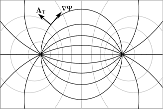
Figure 1: An example of two adjacent regions of positive and negative ${\bf B}\!\cdot\!{\bf n}=-\triangle_{T}\Psi$ on the boundary. The grey lines are contours of the potential $\Psi$ defined by (15). They coincide with field lines of ${\bf A}_{T}$. In black field lines of $\nabla\Psi$ are shown.

The representation (15) can now be used to prove that the difference between the two integrals in (14)vanishes:

$$\int_{V}\nabla\!\cdot\!\left({\bf A}^{a}\times{\bf A}^{b}\right)dV = \int_{\partial V}\left({\bf A}^{a}\times{\bf A}^{b}\right)\!\cdot\!{\bf n}\ da$$

$$= \int_{\partial V}\left(\nabla\Psi^{a}\times\nabla\Psi^{b}\right)\!\cdot\!{\bf n}\ da$$

$$= \int_{\partial V}\left(\nabla\times\Psi^{a}\nabla\Psi^{b}\right)\!\cdot\!{\bf n}\ da=0.$$

Here the last integral vanishes due to the application of Stokes theorem to a surface without boundary.

Furthermore, the universal helicity is additive with respect to complementary volumes. Complementary here describes that the volumes $V^{a}$ and $V^{b}$ are adjacent to one another, and that they satisfy $B^{a}_{n}=B^{b}_{n}$ on their common boundary, and have $B^{a}_{n}=B^{b}_{n}=0$ on all other boundaries. Note that this still assumes that the volumes are simply connected and have no holes. Thus, the total volume $V^{a}\cup V^{b}$ has vanishing normal magnetic field on its boundary, and we can calculate its (classical) total helicity

$$H_{V^{a}\cup V^{b}}({\bf B}^{a}+{\bf B}^{b})=H_{V^{a}}({\bf B}^{a})+H_{V^{b}}({\bf B}^{b}).$$ (19)

The proof relies on the fact that the total helicity on the left hand side is gauge invariant, so that we can choose a gauge for the vector potential such that $\nabla_{T}\!\cdot\!{\bf A}_{T}=0$ holds both on its boundary and on the interface between $V^{a}$ and $V^{b}$. Then the total vector potential can be split in two parts with ${\bf A}^{a}={\bf A}|_{V^{a}}$ (${\bf A}^{a}=0$ on $V^{b}$) and ${\bf A}^{b}$ analogously defined. This implies (19).

IV Interpretation and Example

In the following we prove that the boundary condition $\nabla_{T}\cdot{\bf A}_{T}=0$ corresponds to the existence of a unique field ${\bf B}^{b}$ in the exterior domain $V^{b}$ such that ${\bf A}^{b}\cdot{\bf B}^{b}\equiv 0$. Thus the univeral helicity integral $H_{V^{a}}({\bf B}^{a})$ equals the total helicity integral of ${\bf B}^{a}$ completed by ${\bf B}^{b}$ as Eq. (19) shows. In order to see this we use a coordinate system as introduced for the representation (9) and define ${\bf A}^{b}$ in a layer of thickness $\epsilon$ from the boundary with $f(u_{3})$ as defined in (12):

$${\bf A}^{b} = {\bf A}_{T}(u_{1},u_{2})f(u_{3})$$ (20)

$${\bf B}^{b} = B_{n}(u_{1},u_{2})f(u_{3}){\bf u}^{3}+\frac{\partial f(u_{3})}{\partial u_{3}}\nabla\Psi(u_{1},u_{2})$$ (21)

One easily checks that this satisfies ${\bf A}^{b}\cdot{\bf B}^{b}\equiv 0$. Note that the field ${\bf B}^{b}$ is tangent to surfaces spanned by ${\bf u}_{3}$ and $\nabla\Psi$. Such a surface is shown in Fig. 2.

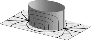
Figure 2: A flux surfaces of the field ${\bf B}^{b}$ derived from (20) for the same boundary condition as used in Fig. 1.

In the limit of $\epsilon\rightarrow 0$ the field ${\bf B}^{b}$ becomes a singular ”surface field”,

$${\bf B}^{b}=B_{n}(u_{1},u_{2})H(-u_{3}){\bf u}^{3}-\delta(u_{3})\nabla\Psi(u_{1},u_{2})\ .$$ (22)

Here $\delta(x)$ is the Dirac delta function and $H(x)$ the Heaviside function. That is, ${\bf B}^{b}$ is a field of finite magnetic flux in the surface, which diverts the normal component $B_{n}$ in a field along $\nabla\Psi$. This field is uniquely determind by the boundary condition.

Example.

For a non-trivial example, consider a field consisting of two untwisted flux tubes with the same magnetic flux $\Phi$ as shown in Fig. 3(a). There are no closed field lines in the volume under consideration, so there is no way of calculating the helicity of this configuration with the classical helicity integral. The configuration of the singular boundary field is shown in Fig. 3(b). An explicit calculation yields $H_{V}({\bf B})=-\Phi^{2}$. This can be understood as the helicity of the closed field shown in Fig. 4(a), which shows a closure of the field with a configuration topologically equivalent to the singular boundary field. The closed tube has a uniform twist of $-2\pi$ and thus a total helicity of $H_{V}({\bf B})=-\Phi^{2}$.

Another way of calculating $H_{V}({\bf B})$ is to make use of the symmetry of the configuration and use Eq. (19). Fig. 4 shows one example. The magnetic field is closed with an identical copy in $V^{\prime}$. This configuration has a total helicity of $-2\Phi^{2}$ due to the linkage of the two flux tubes (see e.g. Berger and Field (1984)). Hence $-2\Phi^{2}=H_{V^{\prime}}({\bf B})+H_{V}({\bf B})$$=2H_{V}({\bf B})$ and therefore $H_{V}({\bf B})=-\Phi^{2}$.

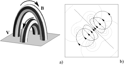
Figure 3: a) The example under consideration and b) the corresponding boundary with contours of $\Psi$ (gray) and field lines of $\nabla\Psi$ (black).

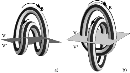
Figure 4: a) The field shown in Fig. 3 is closed by two loops which are topological equivalent to the singular boundary field. b) A closure of the field with $H_{V^{\prime}}({\bf B})=H_{V}({\bf B})$.

V Summary

In this letter it was shown how the total helicity integral can naturally be generalized to allow for magnetic fields which are not closed within the domain, i.e. which have a non-vanishing normal component on the boundary. The construction does not require an explicit reference field as the relative helicity integral does, which was previously used in this situation. Instead we have a gauge condition for ${\bf A}$ on the boundary which corresponds to closing the domain with a topologically unique field. This field is an external complement with zero helicity density to the field in the given domain. The new integral has all desirable properties, i.e. it is gauge invariant, topologically invariant, and it reduces to the total helicity whenever the latter is well defined. Moreover, it shows the proper additivity with respect to fields and complementary volumes. This facilitates not only many calculations of helicity, but also its interpretation.