Neutral gas density in Damped Lyman $\alpha$ systems

Abstract

Accepted for publication in the Astrophysical Journal
We estimate the intrinsic neutral gas density in Damped Lyman $\alpha$ systems ($\Omega_{HI}^{(DLA)}$) in the redshift range $2.2\lesssim z\lesssim 5$ from the DLA SDSS DR_3 sample of optically selected quasars. We take into account self-consistently the obscuration on background quasars due to the dust present in Damped Lyman $\alpha$ systems. We model the column density and redshift distribution of these systems by using both a non-parametric and a parametric approach. Under conservative assumptions on the dust content of Damped Lyman $\alpha$ systems, we show that selection effects lead to underestimating the intrinsic neutral gas density by at least $15\%$ with respect to the observed neutral gas density. Over the redshift range $[2.2;5.5]$ we find $\Omega_{HI}^{(DLA)}=0.97^{+0.08+0.28}_{-0.06-0.15}\cdot 10^{-3}$, where the first set of error bars gives the $1\sigma$ random errors and the second set gives the modeling uncertainty dependent on the fraction of metals in dust - from 0% to 50%. This value compares with $\Omega_{HI}^{(DLA)}=0.82^{+0.05}_{-0.05}$ ($1\sigma$ error bars), which is obtained when no correction for dust is introduced. In the model with half of the metals mass in dust we cannot constraint $\Omega_{HI}^{(DLA)}$ at a confidence level higher than $90\%$. In this case there is indeed a probability of about $10\%$ that the intrinsic column density distribution of DLA systems is a power law $f(N_{HI})\propto 1/N_{HI}^{~{}1.95}$. In contrast, with $25\%$ of the metals in dust - the most realistic estimate - a power law is ruled out at $99.5\%$ of confidence level.

1 Introduction

Damped Lyman $\alpha$ systems (hereafter DLA systems) are quasar absorption systems with a column density above $2\cdot 10^{20}cm^{-2}$ and represent the high end of the distribution of absorption systems starting from the Lyman $\alpha$ forest at $N_{HI}\gtrsim 10^{14}cm^{-2}$. DLA systems represent the most significant reservoir of neutral hydrogen in the universe available for star formation. These systems are considered to be either (cold) massive rotating disks, the progenitors of todays disk galaxies (Prochaska & Wolfe, 1997; Wolfe et al., 2005) or compact protogalactic clumps (Haehnelt et al., 1998; Nagamine et al., 2004).

In the era of precision cosmology, an accurate measure of the total mass density of neutral gas as a function of the redshift represents an important constraint for galaxy formation models. Ground observations are able to identify DLA absorption features in the spectra of quasars from $z_{abs}\gtrsim 1.8$, where the absorption lines enter the atmospheric window, up to $z_{abs}\approx 5.5$. With an all sky survey like the Sloan Digital Sky Survey, spectra of several thousands of quasars with enough resolution for DLA detection have been acquired and the observed density of neutral gas in DLA systems is now measured with errors below $10\%$ (Prochaska et al., 2005).

This measurement must be interpreted with some caution, as the presence of DLA systems along a line of sight leads to a potential obscuration due to the dust that they host: the observed gas density is a biased estimator of the intrinsic density unless the dust effects are accurately quantified. Several papers, starting from Ostriker & Heisler (1984) have attempted to model the influence of dust along the line of sight, often with conflicting results.

A detailed analysis framework for the obscuration of quasars has been developed by Fall & Pei (1993) (see also Fall & Pei 1989; Fall et al. 1989; Pei et al. 1991; Pei & Fall 1995) and applied to the quasars sample of Lanzetta et al. (1991). Their study highlighted a potentially severe effect of the dust bias that did not allow to put an upper limit to the intrinsic density of DLA systems. In fact, absorbers with high column densities and/or with high dust-to-gas ratio represent essentially “bricks” along the line of sight to a quasar and are very likely to be missed in optically selected surveys. An additional evidence for the dust obscuration came in the form of a detected preferential reddening in the spectra of quasars with DLA absorption with respect to a control sample without detection of these systems (Pei et al., 1991).

More recent investigations revised these earlier results on the dust content in DLA systems and on their reddening of background objects (Murphy & Liske, 2004; Ellison et al., 2005), finding in particular no robust evidence for the reddening of quasars at $z\approx 3$ with DLA features in their spectra: at $3\sigma$ Murphy & Liske (2004) find $E(B-V)<0.02mag$, while Ellison et al. (2005) have $E(B-V)<0.04mag$ . At the same time radio selected quasars surveys (Ellison et al., 2001), with complete optical follow-up detection have provided the first bias free constraints on the intrinsic distribution of DLA systems.

Taking advantage of these recent measurements for the number density of DLA systems, we have previously characterized (Trenti & Stiavelli, 2006) the dust absorption along random lines of sight by means of a Monte Carlo code, finding that, on average, the deviations from unit transmission are effectively modest ($\langle\exp{(-\tau)}\rangle\gtrsim 0.9$ at an emitted wavelength $\lambda_{e}=0.14\mu m$ over all the redshift range) and of limited impact on most observations. However, this result does not exclude the presence of a small fraction of lines of sight (of the order of a few percent) through the most massive and/or the most metal-rich DLA systems and characterized by a large optical depth. Indeed, Wild & Hewett (2005) and Wild et al. (2006) find a significant evidence of reddening in DLA systems with CaII absorption lines at moderate redshift ($z_{abs}\approx 1$; $\langle E(B-V)\rangle\gtrsim 0.1$). Similarly York et al. (2006) measure $E(B-V)$ up to 0.085 for MgII selected DLA systems at $z_{abs}\approx 1.0$. As the determination of the gas density in DLA systems is dominated by these most massive absorbers, the potential bias in this measure, correctly stressed by Fall & Pei (1993), must not be dismissed by the recent evidence of a very modest average deviation from unity transmission.

In this paper we take advantage of the large sample of DLA systems identified in Sloan quasars (Prochaska et al., 2005) and we investigate the relation between the observed and intrinsic density of neutral gas in these systems. The Sloan sample that we consider has three main advantages over the sample used by Fall & Pei (1993). (1) It is larger by a factor 30. (2) The quasars have been selected within a luminosity limit in the I band, significantly less sensitive to dust obscuration than the B band used for the older sample. (3) The color selection algorithm has a good sensitivity to red quasars (Richards et al., 2002). In fact even if a quasar with a DLA absorption system is not dropped below the I-band flux limit, its color can be changed so that it ends up lying outside the color selection box used to identify quasar candidates for follow-up spectroscopy. Thanks to the precision of the Sloan photometry, that allows a clear separation of the stellar locus in the color space, and to the use of an extended color selection box, the loss of completeness due to this latter effect is only marginal (see Richards et al. 2002 for a detailed discussion of the Sloan color selection algorithm and for completeness tests) and is therefore not considered in this work.

This paper is organized as follows. In Sec. 2 we characterize the obscuration bias in a magnitude limited survey, in Sec. 3 we describe the dataset that we are using. In Sec. 4 we present our analysis for the parametric estimation of the intrinsic comoving density of neutral gas, whose uncertainties are quantified in Secs. 5-6 by means of Monte Carlo simulations of synthetic observations. In Sec. 7 we discuss the accuracy of a non-parametric estimator for the neutral gas density. We summarize our findings in Sec. 8.

2 Dust effects in magnitude limited surveys

In a magnitude limited survey, obscuration along the line of sight leads to the potential loss of some lines of sight. Following Fall & Pei (1993), to quantify the effect let us consider an intrinsic quasar luminosity function $\Phi_{i}(L)$ in the interval $[L_{min},+\infty]$, where $L_{min}$ is the luminosity above which the sample is complete. The intrinsic number of objects above the completeness threshold is:

$$N_{i}=\int_{L_{min}}^{+\infty}\Phi_{i}(L)dL.$$ (1)

The presence of dust introduces an optical depth $\tau$ along the line of sight, with a corresponding transmission coefficient $\exp{\{-\tau\}}$. Under this condition the number of objects with observed luminosity above $L_{min}$ is:

$$N_{o}=\int_{L_{min}e^{\tau}}^{+\infty}\Phi_{i}(L)dL.$$ (2)

The dust obscuration leads to a fraction of missing objects given by $N_{o}/N_{i}$:

$$\frac{N_{o}}{N_{i}}=\frac{\int_{L_{min}e^{\tau}}^{+\infty}\Phi_{i}(L)dL}{\int_{L_{min}}^{+\infty}\Phi_{i}(L)dL}$$ (3)

In general the precise value of $N_{o}/N_{i}$ for a given $\tau$ depends on the sensitivity limit of the survey $L_{min}$ and on the form of the luminosity function $\Phi(L)$. Under the assumption that the luminosity function is a power law $\Phi(L)\propto L^{-\beta-1}$ (in the luminosity range from $L_{min}$ to $+\infty$) the ratio $N_{o}/N_{i}$ can be easily computed and is independent of $L_{min}$:

$$\frac{N_{o}}{N_{i}}=\frac{L_{min}^{-\beta}e^{-\beta\tau}}{L_{min}^{-\beta}}=e^{-\beta\tau}.$$ (4)

This was already noted by Fall & Pei (1993).

The luminosity function for quasars is modeled in terms of a gamma function and/or of a double power law (e.g., see Pei, 1995). However the SDSS spectroscopic quasar sample is shallower, for $z_{qso}\gtrsim 2.2$, than the knee of the distribution so that the luminosity function for the quasars that we are considering in this paper can be effectively treated up to $L_{min}$ as a single power law (see Richards et al., 2006), simplifying significantly our analysis by use of Eq. (4).

In the following analysis we assume a redshift dependent luminosity function (Richards et al., 2006):

$$\Phi_{i}(L_{i},z)=A(z)L_{i}^{-\beta(z)-1},$$ (5)

where $L_{I}$ is the luminosity in $I$ band (where the sensitivity limit for detection of quasars in SDSS is given) and $\beta(z)$ is a slowly evolving function of the redshift with $\beta$ varying from 2.2 to 1.1 in the redshift range $[2;5]$ (Richards et al., 2006):

$$\beta(z)=2.1-0.275(z-2.45)\theta(z-2.45),$$ (6)

where $\theta(x)$ is the step function defined as $\theta(x)=1$ if $x\geq 0$ and $\theta(x)=0$ otherwise. The SDSS DLA DR_3 sample of quasars considered in this paper has an average redshift of $2.97$ with a standard deviation of $0.65$. The average slope can be approximated as:

$$\langle\beta\rangle=1.95\approx 2.$$ (7)

In case of absorption due to a dusty DLA system at redshift $z_{a}$ with column density $N_{HI}$, the optical depth at an observed wavelength $\lambda_{o}$ can be written as:

$$\tau(\lambda_{o},z_{a},N_{HI},k)=kN_{HI}\xi(\lambda_{o}/(1+z_{a})),$$ (8)

where $k$ is the dust-to-gas ratio and $\xi$ the relative extinction curve normalized to the absorption cross section in B band $\sigma(\lambda_{B})$ (e.g., see Pei, 1992):

$$\xi(\lambda)=\sigma(\lambda)/\sigma(\lambda_{B}).$$ (9)

If $N_{HI}$ is expressed in units of $10^{21}cm^{-2}$, the absorption cross section in B band is $kN_{HI}$ with $k=0.8$ for galactic dust. The value of $k$ for DLA systems depends on their metallicity $Z$ and on the fraction of metals in dust, i.e. on the dust-to-metals ratio. DLA systems are generally characterized by a low metallicity and by a moderate evolution of their properties with the redshift (Wolfe et al., 2005). We approximate the observed average (HI-column density weighted) redshift-metallicity relation (based on a number of observations, e.g. Prochaska et al. 2003, Dessauges-Zavadsky et al. 2004, 2006, Akerman et al. 2005) with a linear function for $\log{(Z_{o}(z))}$. This provides a good agreement with the data (e.g. see Fig. 13 in the compilation by Kulkarni et al. 2005) in the redshift range $2\lesssim z\lesssim 5$:

$$Z_{o}(z)/Z_{\sun}=0.2\cdot 10^{-0.2z}.$$ (10)

The average metallicity in Eq. (10) translates, for a Milky Way dust-to-metals ratio (i.e. $50\%$ of the metals in dust grains), into a “Milky Way” average dust-to-gas ratio:

$$k_{MW}(z)=0.16\cdot 10^{-0.2z}.$$ (11)

To account for different fractions of metals in the form of dust grains we introduce a correction factor $\alpha_{\kappa}$ for the intrinsic dust-to-gas ratio $k_{i}(z)$:

$$k_{i}(z)=\alpha_{\kappa}k_{MW}(z).$$ (12)

DLA systems are considered to have a smaller fraction of metals in dust than our galaxy (with roughly one quarter of the total metals content in dust), so realistic values for $\alpha_{\kappa}$ are expected to be around $\alpha_{\kappa}=0.5$ (Pettini et al. 1997; Vladilo 2002; but see Pei et al. 1999 where the Milky Way dust-to-metals ratio is used). In the following sections we present our analysis using a range of dust-to-metals ratio, highlighting the dependence of the dust bias on this quantity. We assume a reference value $\alpha_{\kappa}=0.5$ (25% of metals in dust, the value derived by Pettini et al. 1997), but we include a grid of models with $\alpha_{\kappa}\in[0;1]$ with $\Delta\alpha_{\kappa}=0.125$, discussing in depth also the case $\alpha_{\kappa}=1$ (50% of metals in dust).

Our analysis is carried out by assuming that all DLA at a given redshift have a fixed metallicity, as well as a fixed dust-to-metals ratio. A detailed modeling of the metallicity and dust-to-metals ratio distributions for the purpose of determining $\Omega_{HI}^{(DLA)}$ is extremely challenging, as only a small subsample of DLA system have measured metallicities. Fortunately, the value of $\Omega_{HI}^{(DLA)}$ is not expected to significantly depend on the scatter in the dust-to-gas ratio $k_{i}$ of the absorbers (see Fall & Pei 1993, Appendix A). To ensure that this is the case, in Sec. 6 we validate our scatter-less approach by analyzing synthetic observations with a variety of dust-to-gas distributions.

3 The data: The DLA SDSS DR_3 and the CORALS surveys

The data used in this paper are primarily taken from the DLA survey by Prochaska et al. (2005). We consider all the quasars from their Table 1 and all the DLA systems reported in their Table 3. The sample consists of 525 DLA system found in 4568 spectra of quasars with a minimum signal to noise ratio of 4.

In addition we consider the DLA systems detections in the radio selected CORALS survey (Ellison et al., 2001), intrinsically free from dust bias. This survey consists of 19 DLA systems detected in 66 spectra of quasars (see their Table 3). The statistical sample for the survey (see Ellison et al. 2001), that we consider for the analysis, is restricted to $17$ DLA in the redshift range $[1.8;3.5]$.

4 Parametric Estimation of $\Omega_{HI}^{(DLA)}$ from SDSS DR3

Following the standard practice (e.g. Lanzetta et al. 1991) we define the number of observed DLA systems in the intervals $[N_{HI},N_{HI}+dN_{HI}]$ and $[X,X+dX]$:

$$f_{o}(N_{HI},X)dN_{HI}dX,$$ (13)

where $f_{o}$ is the observed frequency distribution and $dX$ the absorption distance:

$$dX\equiv\frac{H_{0}}{H(z)}(1+z)^{2}dz.$$ (14)

In this paper we adopt the standard $\Lambda CDM$ cosmology with $H_{0}=70km/s/Mpc$, $\Omega_{\Lambda}=0.7$ and $\Omega_{M}=0.3$, so that:

$$dX=\frac{(1+z)^{2}}{\sqrt{0.7+0.3(1+z)^{3}}}dz.$$ (15)

The data from SDSS DLA DR_3 span over a total integrated absorption path-length $\Delta X=7333.1$.

Considering the obscuration bias discussed in the previous section for the Sloan survey (see also Fall & Pei 1993) and assuming that the distribution of absorbers along the line of sight is not correlated, we can write the relation between the intrinsic and the observed frequency distribution of DLA systems as:

$$f_{o}(N_{HI},z)=f_{i}(N_{HI},X(z))e^{-\langle\beta\rangle\alpha_{\kappa}k_{MW}(z)N_{HI}\xi(\lambda_{I}/(1+z))},$$ (16)

where we assume the average slope $\langle\beta\rangle=2$ for the quasar luminosity function. Following Prochaska et al. (2005) we parameterize $f$ using a gamma function:

$$f_{i}(N_{HI},X)=\eta_{1}\left(\frac{N_{HI}}{N_{\gamma}}\right)^{m_{1}}\exp{\left(-\frac{N_{HI}}{N_{\gamma}}\right)},$$ (17)

and a power law:

$$f_{i}(N_{HI},X)=\eta_{2}\left({N_{HI}}\right)^{m_{2}}.$$ (18)

The use of the gamma function for the intrinsic distribution $f_{i}$ has the advantage that, given Eq. (16), also the observed distribution $f_{o}$ remains a gamma function. A intrinsic power law is instead mapped into a observed gamma function by the effect of dust.

If we assume that the intrinsic distribution of DLA systems follows a Poisson statistics, the observed distribution will also follow a Poisson statistics. The likelihood to be maximized is therefore (see also Eq. 27 in Fall & Pei 1993):

$$\mathcal{L}=\exp{-\left\{\sum_{s}\int_{{z_{inf}}_{s}}^{{z_{sup}}_{s}}dz\int_{N_{DLA}}^{+\infty}dN_{HI}\cdot f_{o}({N_{HI}}_{s},z_{s})\frac{dX}{dz}\right\}}\prod_{n}f_{o}({N_{HI}}_{n},z_{n}),$$ (19)

where the sum extends over all the sample of quasars that have been searched for DLA systems in the redshift interval $[{z_{inf}}_{s};{z_{sup}}_{s}]$, where the signal to noise ratio is above $4$, and the product is over all the DLA systems detected in those quasars. In Eq. (19) the observed distribution function $f_{o}$ is expressed in terms of the intrinsic distribution $f_{i}$ through Eq. (16). $N_{DLA}=2\cdot 10^{20}cm^{-2}$ is the assumed lower limit for the column density of a DLA system.

Before presenting the results from the maximum likelihood analysis we investigate the properties of $f_{o}$ with the aim to discuss upper limits on the dust-to-gas ratio and on $\Omega_{HI}^{(DLA)}$.

4.1 Basic considerations from the properties of $f_{o}$

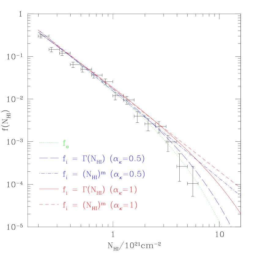
Figure 1: Observed column density distribution of DLA systems in the SDSS DLA DR_3 sample compared to observed (solid) and intrinsic (dotted) best fitting gamma functions. The difference between $f_{i}$ and $f_{o}$ is due to dust obscuration, especially apparent for high column densities. The parameters value for the fitting functions are reported in Tables. 1-2.

Fig. 1 shows the observed column density distribution of DLA systems, averaged over redshift. The observed data are well fitted by a gamma function (Prochaska et al. 2005, see also Eq. 17 and Tab. 1) with a knee at $(N_{\gamma})_{o}=3\cdot 10^{21}cm^{-2}$ and a slope $(m_{1})_{o}=-1.8$.

The origin of the observed knee at $(N_{\gamma})_{o}$ can in principle be either due to an intrinsic decrease of the distribution at high column densities, i.e. due to $N_{\gamma}$, or due to the effect of obscuration bias, that introduces in the data an exponential-like decrease. We can obtain a limit on the dust-to-gas (expressed in terms of $\alpha_{\kappa}$) ratio assuming that the observed knee is entirely due to dust bias. From Eq. (16) we can write:

$$\langle\beta\rangle\alpha_{\kappa}k_{MW}(z)\xi(\lambda_{I}/(1+z))\lesssim 1/(N_{\gamma})_{o},$$ (20)

so that, considering that the average redshift of DLA absorbers in our sample is $\langle z\rangle=3.1$ we estimate a limit on $\alpha_{\kappa}$:

$$\alpha_{\kappa}\lesssim\frac{1}{(N_{\gamma})_{o}}\cdot\frac{1}{\langle\beta\rangle k_{MW}(\langle z\rangle)\xi(\lambda_{I}/(1+\langle z\rangle))}\lesssim\frac{1}{3}\cdot\frac{1}{2\cdot 0.038\cdot 2.47}\lesssim 1.75.$$ (21)

As this value implies about $90\%$ of metals in dust, which appears extremely improbable for DLA systems, the presence of an observed knee in the column density distribution of the gas is likely an intrinsic feature and not induced by the dust bias alone. This implies that the expected difference between the intrinsic and the observed density of neutral gas in DLA systems is limited for the most realistic fraction of metals in dust ($25\%$ i.e. $\alpha_{\kappa}=0.5$). Only in the case of a larger fraction of metals in dust (i.e. $\alpha_{\kappa}\approx 1$) there can be the possibility of a significant dust bias, as in that case an acceptable model of the intrinsic distribution can still be obtained in terms of a power law. In the next Section we quantify more precisely the dust bias by studying the likelihood $\mathcal{L}$ for $f_{i}$ at increasing $\Omega_{HI}^{(DLA)}$ for different values of $\alpha_{\kappa}$.

4.2 Whole sample analysis

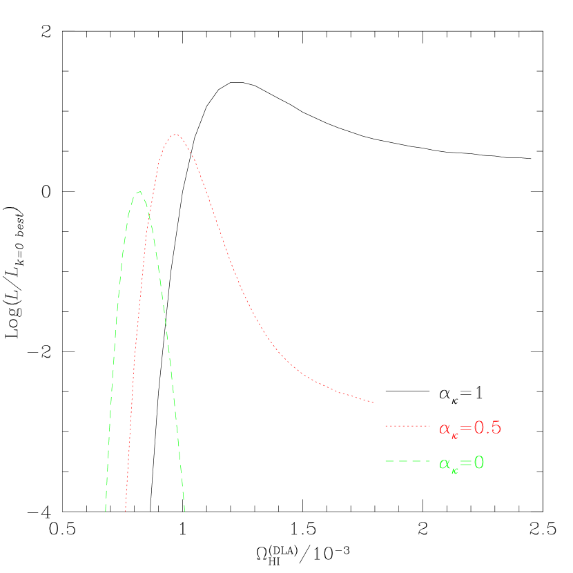
Figure 2: Maximum likelihood $\mathcal{L}$ for the intrinsic comoving neutral gas density in DLA systems $\Omega_{HI}^{(DLA)}$ for the SDSS DLA DR_3 data (solid line with $\alpha_{\kappa}=1$; red dotted with $\alpha_{\kappa}=0.5$ ). The green dashed line is associated to the observed gas density ($\alpha_{\kappa}=0$). The likelihood curves have been obtained by maximizing $\mathcal{L}$ over $N_{\gamma}$ and $m_{1}$ at fixed $\Omega_{HI}^{(DLA)}$ and $\alpha_{\kappa}$.

By aggregating all the data in SDSS DLA DR_3, the results of our maximum likelihood analysis are reported in Tables 1-2 and in Fig. 2. The results for the fit with an intrinsic gamma function are reported in terms of the comoving density of gas in DLA systems (${\Omega_{HI}^{(DLA)}}$), that is the first moment of $f_{i}$:

$${\Omega_{HI}^{(DLA)}}dX=\frac{\mu m_{H}H_{0}}{c\rho_{c}}\int_{N_{DLA}}^{+\infty}dN_{HI}N_{HI}f_{i}(N_{HI},z)dX,$$ (22)

where $m_{H}$ is the mass of the hydrogen atom, $\mu=1.3$ is a correction factor for the composition of the gas, $c$ the speed of light, $\rho_{c}$ the critical density and $N_{DLA}=2\cdot 10^{20}cm^{-2}$.

We obtain the following results:

• $\alpha_{\kappa}=0$: If we neglect the effect of dust absorption so that $f_{o}\equiv f_{i}$, we re-derive the parameters for the gamma distribution reported in Prochaska et al. (2005) (see our Tab. 1). All our likelihood values for the Sloan data are presented in log units normalized to the likelihood value for the best fitting dust-free model. For $\alpha_{\kappa}=0$ the likelihood is sharply peaked around the best value for $\Omega_{HI}^{(DLA)}$. However, when we introduce the effect of the dust ($\alpha_{\kappa}>0$) there is an increasingly strong degeneration toward high values for $\Omega_{HI}^{(DLA)}$ (see Fig. 2).

• $\alpha_{\kappa}=0.5$: For our standard scenario the likelihood has a maximum at $\Omega_{HI}^{(DLA)}=0.97\cdot 10^{-3}$, to be compared with the value $\left(\Omega_{HI}^{(DLA)}\right)_{0}=0.82\cdot 10^{-3}$ given by the maximum likelihood analysis with $\alpha_{\kappa}=0$ (no dust). In our modeling of the column density distribution the metallicity is introduced has an external input, based on independent observations. An additional support to motivate the need of taking into account the obscuration bias comes from the fact that the likelihood for $\alpha_{\kappa}=0.5$ is higher than for $\alpha_{\kappa}=0$.

• $\alpha_{\kappa}=1$: The bias induced by the dust increases as larger $\alpha_{\kappa}$ are considered. As expected qualitatively by the simple considerations on the shape of $f_{o}$ presented in the previous section, the maximum likelihood analysis for our large dust-to-metal ratio scenario ($\alpha_{\kappa}=1$) is unable to set a strong upper limit to $\Omega_{HI}^{(DLA)}$ as there is a wide wing of high likelihood values toward large neutral gas densities. At $\alpha_{\kappa}=1$ a power law $f_{i}$ with slope $m_{2}=-1.95$ has a likelihood ratio over the best gamma solution of $\mathcal{R}=2\log({\mathcal{L}}_{\Gamma}/{\mathcal{L}}_{N^{m}})=2.1$. A likelihood ratio test with this value implies that a power law solution can be ruled out only at about 85% of confidence level if we assume that $\mathcal{R}$ is distributed as a $\chi^{2}$ with one degree of freedom. However this is in general valid only when the model is linear in the parameters and the errors follow a gaussian distribution (Lupton, 1993). As our model is strongly non linear, in the next section we estimate the confidence level by means of Monte Carlo simulations.

• $\alpha_{\kappa}>1$: If we consider fits for $f_{i}$ at $\alpha_{\kappa}>0$ (see Table 2) we obtain an increasingly better modeling in terms of power laws up to $\alpha_{\kappa}\approx 2$. As expected from the preliminary examination of $f_{o}$, eventually the likelihood decreases at higher dust-to-gas ratio starting from $\alpha_{\kappa}\gtrsim 2$. We recall that $\alpha_{\kappa}>2$ is formally unphysical, as it implies more than 100% of the metals in dust, however, due to the fact that we have adopted a simple fit to the observed metallicity, a high $\alpha_{\kappa}$ value also means that the intrinsic metallicity content of DLA system is underestimated in our model. As it appears unlikely that the metallicity measurements do significantly underestimate the dust content of DLA systems, we expect that realistic values of $\alpha_{\kappa}\leq 1$.

• CORALS: For comparison we have repeated the maximum likelihood analysis on the radio selected CORALS quasars (Ellison et al., 2001). The results are reported in Table 3 and in Fig. 3. For these data the measure is guaranteed to be free from dust bias, but the sample size is insufficient to accurately constraint the parameters of $f_{i}$ (the likelihood curve in Fig. 3 is relatively flat around the maximum). The maximum is at $\Omega_{HI}^{(DLA)}=1.2\cdot 10^{-3}$ with extremely large $1\sigma$ uncertainties (of the order of 50%) due to the flatness of the likelihood function. In addition, the maximum likelihood for the gamma function model is only negligibly better than the one for a power law ($\mathcal{R}\approx 0.1$).

5 Errors estimate

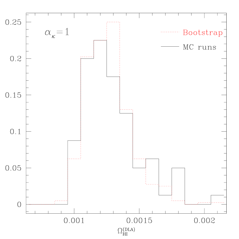
Figure 4: $\Omega_{HI}^{(DLA)}$ distribution for $\alpha_{\kappa}=1$ from the bootstrapping analysis of the data (red dotted line; 400 realizations) and from 80 Monte Carlo realizations (solid line) of synthetic observations starting from the best fitting model for $f_{i}$ (gamma function with $m_{1}=-1.8$, $N_{\gamma}=7.22\cdot 10^{21}cm^{-2}$ and $\Omega_{HI}^{(DLA)}=1.25\cdot 10^{-3}$).

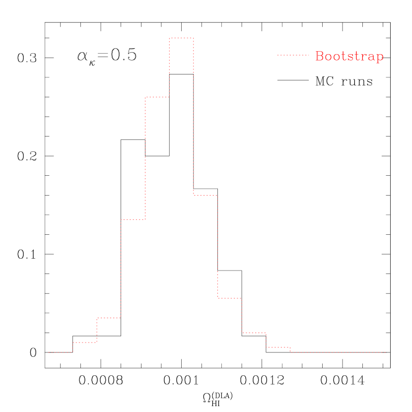
Figure 5: $\Omega_{HI}^{(DLA)}$ distribution for $\alpha_{\kappa}=0.5$ from the bootstrapping analysis of the data (red dotted line; 200 realizations) and from 60 Monte Carlo realizations (solid line) of synthetic observations starting from the best fitting model for $f_{i}$ (gamma function with $m_{1}=-1.79$, $N_{\gamma}=4.15\cdot 10^{21}cm^{-2}$ and $\Omega_{HI}^{(DLA)}=0.97\cdot 10^{-3}$).

To estimate the error on the determination of $\Omega_{HI}^{(DLA)}$ we have performed a bootstrapping analysis of the data. We have randomly extracted samples of lines of sight with uniform probability from the SDSS DLA survey. The samples have the same number of lines as the original data. For each of these simulated samples we have performed a maximum likelihood analysis to determine $\Omega_{HI}^{(DLA)}$. In the case of $\alpha_{\kappa}=1$, the results obtained with 400 random realizations are presented in Fig. 4 and show that $\Omega_{HI}^{(DLA)}$ is indeed distributed around the best value derived from the original data ($1.25\cdot 10^{-3}$), which coincides with the median of the distribution. The average value of the distribution is $1.27\cdot 10^{-3}$. At $68\%$ of confidence level the measurements lie in the interval $[1.10\cdot 10^{-3};1.41\cdot 10^{-3}]$. We assume this interval as our fiducial error on $\Omega_{HI}^{(DLA)}$. At $90\%$ of confidence level $\Omega_{HI}^{(DLA)}\leq 1.48\cdot 10^{-3}$. The bootstrapping procedure has been repeated for all the scenarios with different $\alpha_{\kappa}$, resorting to at least $100$ simulations for each value of the dust-to-metals ratio considered. The results are reported as standard $1\sigma$ error in Table. 1. The case $\alpha_{\kappa}=0.5$ is shown in Fig. 5 (using 200 simulations in this case).

As a additional test to investigate the uncertainties in our analysis, we have simulated a number of synthetic samples of data using the Monte Carlo code developed in Trenti & Stiavelli (2006). These samples have then been processed using the same method applied to the real observed data, to test its efficiency in retrieving the input parameters and to quantify the typical error.

Each random realization of a simulated observation is characterized by the same observed path-length of the SDSS sample ($\Delta X=7333$), but consists of lines of sight with DLA distribution (and detection) in the redshift range $[2.2;4]$ The optical depth along each intrinsic line of sight is computed from the realized DLA distribution and then a test on the obscuration probability (Eq. 4) is performed to accept or reject the intrinsic line of sight as a observed one. The only source of uncertainty in these synthetic observations comes from the discrete sampling of $f_{i}$ and from the obscuration probability test. The model does not include observational errors.

We have simulated two models: (i) an intrinsic gamma function and (ii) an intrinsic power law, with the parameters given by the maximum likelihood analysis from the SDSS data (see Table 1 for the gamma function and Table 2 for the power law).

Fig. 4 shows, for $\alpha_{\kappa}=1$, the distribution of $\Omega_{HI}^{(DLA)}$ as measured from the simulated observations (80 different realizations) of a intrinsic gamma function. It is reassuring that the distribution basically agrees with the one obtained using the bootstrap method. The mean value for $\Omega_{HI}^{(DLA)}$ is $1.29\cdot 10^{-3}$ with a standard deviation of $0.23\cdot 10^{-3}$. As we used an input value $\Omega_{HI}^{(DLA)}=1.25\cdot 10^{-3}$ to generate the synthetic observations, the fitting procedure is able to recover the intrinsic density of neutral gas introducing only a negligible bias, which is much smaller than the one sigma random uncertainty.

The analysis of the simulated observations generated from an intrinsic power law distribution allows to quantify the probability that the identification of a gamma function as best fitting model for the Sloan data is only due to the combined effect of discrete sampling and of the additional degree of freedom of the gamma function over a power law. For our reference scenario ($\alpha_{\kappa}=0.5$) we have generated 400 random realizations of observations starting from an intrinsic power law with unconstrained neutral gas density ($\eta_{2}=1.54\cdot 10^{-2}$, $m_{2}=-2.05$). The likelihood ratio (gamma over power law) distribution shows only 2 realizations that have $\mathcal{R}$ greater than the one measured from the SDSS DLA data. This means that an intrinsic power law can be ruled out at $99.5\%$ of confidence level. Repeating the experiment in the case of $\alpha_{\kappa}=1$, $\eta_{2}=1.77\cdot 10^{-2}$ and $m_{2}=-1.95$ we find that about $8~{}\%$ of the realizations have a value of $\mathcal{R}$ greater than the one measured from the SDSS DLA data. This means that the confidence level at which a power law distribution (with unconstrained upper cut-off) can be ruled out is in this case $92\%$.

6 Synthetic observations with dust-to-gas ratio scatter

In the maximum likelihood applied in this work we assume that all the absorbers have a fixed dust-to-metals ratio $\alpha_{\kappa}$ and a metallicity dependent only on the redshift. In reality a significant scatter around the mean values is expected for both these quantities and has indeed been observed (e.g. see Kulkarni et al., 2005). Fall & Pei (1993) have already noted that the scatter in the dust-to-gas ratio is not introducing significant bias under the assumption that there is no correlation between $k_{i}$ and the column density $N_{HI}$.

To confirm the results of Fall & Pei (1993) and to extend the analysis of the bias to the case where a correlation between $k_{i}$ and $N_{HI}$ is present we have simulated a number of synthetic samples of data adopting an approach similar to the one described in Sec. 5. In this case we compute the optical depth of each absorber by drawing dust-to-gas ratio $k_{i}$ from a given distribution, rather than adopting a fixed value depending only on $z$.

When there is no correlation between $k_{i}$ and $N_{HI}$ we use (based on Eq. 12):

$$k_{i}(z)=\xi\cdot\alpha_{\kappa}\cdot k_{MW}(z),$$ (23)

where $\xi$ is a random variable with a given probability distribution $p(\xi)$ such that the expected value of $\xi$ under $p$ is $E_{p}[\xi]=1$. We have considered the following form for $p(\xi)$:

• A uniform distribution around the average value: $p(\xi)=1$ if $\xi\in[0.5;1.5]$ and $p(\xi)=0$ otherwise.

• A lognormal distribution with variance parameter $\sigma_{*}$, as studied by Fall & Pei (1993): $p(\xi)=\exp{\{-\log^{2}{(\xi\exp{\{\sigma_{*}^{2}/2\}})}}/(2\sigma^{2}_{*})\}/\sqrt{2\pi\sigma^{2}_{*}\xi^{2}}$. We adopt $\sigma_{*}=0.5,1,1.5$ inspired by the dispersion in the dust-to-gas ratio observed for galaxies in the local universe (Pei, 1992).

In addition we have generated synthetic observations with a correlation between $k_{i}$ and $z_{i}$ adopting the following prescription:

$$k_{i}(z)=\xi\cdot N_{HI}^{\gamma}\frac{\int_{N_{DLA}}^{+\infty}dN_{HI}\cdot N_{HI}f_{i}(N_{HI})}{\int_{N_{DLA}}^{+\infty}dN_{HI}\cdot N_{HI}^{1+\gamma}f_{i}(N_{HI})}\cdot\alpha_{\kappa}\cdot k_{MW}(z),$$ (24)

where $\gamma=-0.8,-0.4,0.4,-0.8$ (i.e we explore both a increasing and decreasing trend of $k_{i}$ vs. $N_{HI}$) and $\xi$ is a random variable with the same properties bescribed above. The normalization adopted is such that the HI column density averaged value of $k_{i}$ is $\alpha_{\kappa}\cdot k_{MW}(z)$.

For each combination of the parameters considered (see Table 4), we have generated 60 synthetic SDSS-like samples of data (as in Sec. 5) adopting a gamma function model for $f(N_{HI})$ ($N_{\gamma}=4.15\cdot 10^{21}cm^{-2}$; $m_{1}=-1.8$) and $\alpha_{\kappa}=0.5$. These synthetic samples have all $\Omega_{HI}^{(DLA)}=0.97\cdot 10^{-3}$. By applying our maximum likelihood we obtain the following results (summarized in Table 4):

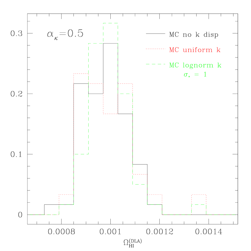
Figure 6: $\Omega_{HI}^{(DLA)}$ distribution from Monte Carlo realizations with a dust-to-gas ratio scatter of synthetic observations starting from the best fitting model for $f_{i}$ (gamma function with $m_{1}=-1.79$, $N_{\gamma}=4.15\cdot 10^{21}cm^{-2}$ and $\Omega_{HI}^{(DLA)}=0.97\cdot 10^{-3}$). The histograms have been constructed using 60 random realizations each. The solid black line is for a model with no scatter, the red dotted line for a model with a uniform dispersion in $k_{i}$ and the green dashed line for a model with a lognormal distribution (with $\sigma_{*}=1$).

• Uncorrelated scatter in $k_{i}$. The maximum likelihood analysis is able to correctly recover the value of $\Omega_{HI}^{(DLA)}$ used to generate the observations (see Fig. 6 and Table 4). There is only a small bias (at the percent level) toward obtaining output values marginally larger than the input, even when the dust obscuration is such that the observed column density averaged dust-to-gas ratio is smaller by $15\%$ with respect to the intrinsic value, as happens in our lognormal model with $\sigma_{*}=1$. This demonstrates that our analysis in terms of the average dust-to-gas ratio is robust with respect to uncorrelated scatter in $k_{i}$. Interestingly we also note that the difference between the observed and the intrinsic dust-to-gas ratio for the lognormal model with $\sigma_{*}=1$ is in agreement with the difference between the metallicity in optically and radio selected samples of DLA systems (see Akerman et al. 2005).

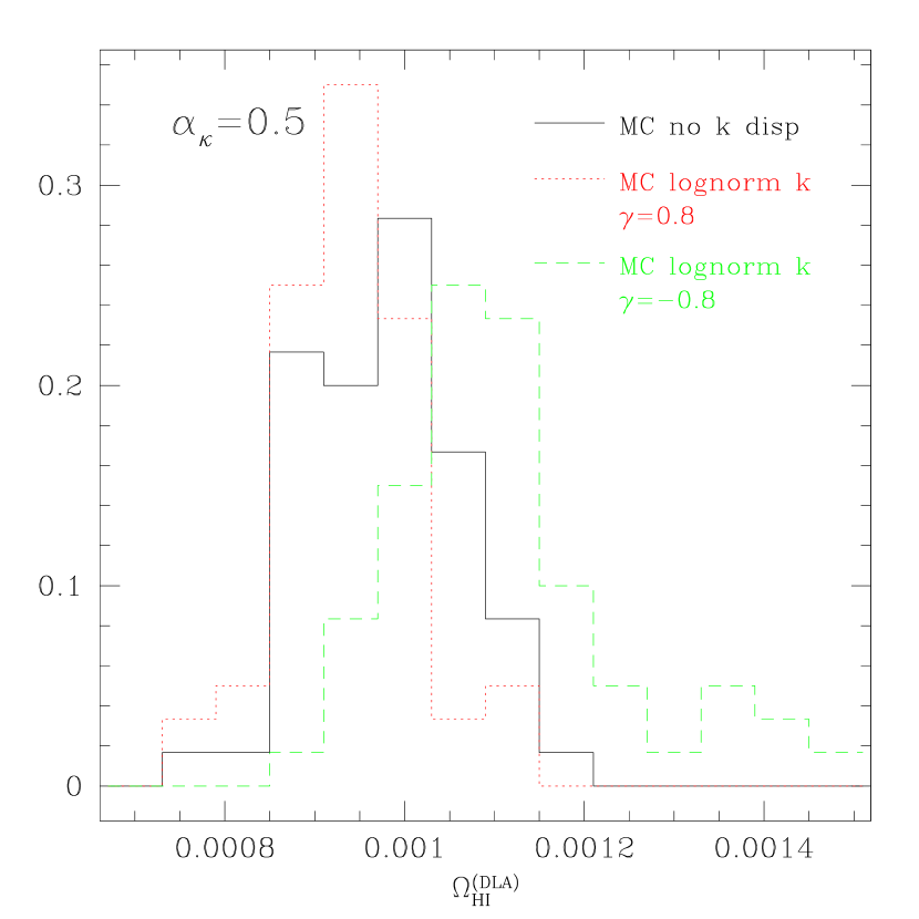
Figure 7: Like fig. 6, but for synthetic observations with a lognormal $k_{i}$ distribution ($\sigma_{*}=1$) and a large correlation ($\gamma=\pm 0.8$) between $k_{i}$ and $N_{HI}$ (green dashed and red dotted lines) vs. realizations with no scatter (black solid line).

• Correlated scatter in $k_{i}$. In this scenario the analysis in terms of an average dust-to-gas ratio systematically mis-estimates the dust content at both ends of the column density distributions of the absorbers. In particular, if $k_{i}$ increases with $N_{i}$, then absorbers with the largest column densities will be more dust rich than assumed by our analysis. This means that these absorbers will more likely be dropped by the sample than is assumed in the modeling, so that $\Omega_{HI}^{(DLA)}$ is underestimated. When $k_{i}$ decreases with $N_{i}$, the opposite happens: the densest absorbers are less dusty than assumed and $\Omega_{HI}^{(DLA)}$ is overestimated. Due to the skewness of the lognormal distribution the bias introduced by the correlation is expected to be larger when $k_{i}$ is a decreasing function of $N_{HI}$. This is indeed what we observe in the analysis of our synthetic observations (see Fig. 7 and Table 4). The bias introduced is, however, relatively modest (at most $15\%$ in $\Omega_{HI}^{(DLA)}$), even assuming a rather strong dependence of $k_{i}$ on $N_{HI}$ (i.e. $k_{i}\propto N_{HI}^{\pm 0.8}$). The bias could be avoided by taking into account the precise form of the correlation into the modeling of the the dust-to-gas ratio. Unfortunately the $k_{i}$ vs. $N_{HI}$ correlation appears hard to quantify with the present data. Only a small subset of the known DLA systems have a measured metallicity and highly dusty and dense absorbers are preferentially missed from the sample. In addition there are some evidences that the fraction of metals depleted in dust depends on the column density of the absorbers (Welty et al., 1997). Therefore plots of the measured gas phase metallicity versus the hydrogen column density, such as those presented in Boisse et al. (1998) and Savaglio (2001) cannot be easily interpreted to extract the $k_{i}(N_{HI})$ relation.

7 Non-parametric Estimation of $\Omega_{HI}^{(DLA)}$ from SDSS DR3

The comoving density of DLA systems can be also estimated using a non-parametric approach by taking the discrete limit of Eq. (22) combined with Eq. (16):

$${\Omega_{HI}^{(DLA)}}=\frac{\mu m_{H}H_{0}}{c\rho_{c}}\frac{\sum_{s}{N_{HI}}_{s}e^{\beta_{s}\tau_{s}}}{(\Delta X)_{i}}.$$ (25)

The sum is done over all the DLA systems in the sample, while the intrinsic total path-length $(\Delta X)_{i}$ is given by summing over all the individual path-lengths for the quasars in the survey, with a weight depending on the optical depth $\tau_{n}$ along the line of sight to the $n-th$ quasar and on the redshift-dependent slope of the quasar luminosity function $\beta(z)$:

$$(\Delta X)_{i}=\sum_{n}(dX_{o})_{n}e^{\beta_{n}\tau_{n}}$$ (26)

The optical depth $\tau_{n}$ is given by:

$$\tau_{n}=\alpha_{\kappa}\sum_{p}k_{MW}(z_{p}){N_{HI}}_{p}\xi(\lambda_{I}/(1+z_{p})),$$ (27)

where the index $p$ is running over all the DLA systems along the $n-th$ line of sight.

The random uncertainty on the measure has been estimated by using a ‘Jack-knife’ analysis (Lupton, 1993): we derive ${\Omega_{HI}^{(DLA)}}$ for $N=22$ subsamples of quasars by ignoring $N_{tot}/N$ quasars each time. The uncertainty on $\Omega_{HI}^{(DLA)}$ is then given by:

$$\sigma^{2}=\frac{N-1}{N}\sum_{s}(\Omega_{s}-\langle\Omega_{s}\rangle)^{2},$$ (28)

where $\Omega_{s}$ stands for ${\Omega_{HI}^{(DLA)}}_{s}$.

We obtain the following results:

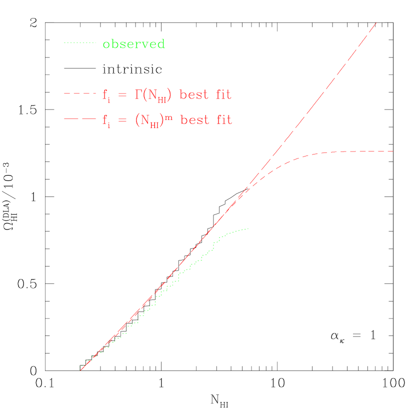
Figure 8: Cumulative neutral gas density in DLA systems versus column density for the SDSS DLA DR_3 (observed dotted, intrinsic with $\alpha_{\kappa}=1$ solid). Superimposed to the intrinsic curve we show the profile from the best fitting gamma function $f_{i}$ (short dashed) and from a power law $f_{i}$ (long dashed) with slope $-1.95$: the discrete evaluation for the intrinsic distribution does not extend to sufficiently high column densities to allow convergence.

• $\alpha_{\kappa}=1$: Eq. 25, applied to the whole sample with $\alpha_{\kappa}=1$, gives $\Omega_{HI}^{(DLA)}=1.04\cdot 10^{-3}$ with an error of $8\cdot 10^{-5}$ (see Table 5). The obscuration bias based on this estimate is of about $30~{}\%$. This represents a lower limit on the bias, as from Fig. 8 it is evident that with $\alpha_{\kappa}=1$ the dust bias is so severe that the discrete evaluation of ${\Omega_{HI}^{(DLA)}}$ has not converged. On the top of the random errors, estimated with the ’Jack-knife’ method, this non parametric estimation suffers from systematic effects of the order of at least $10-20\%$.

• $\alpha_{\kappa}=0.5$: The values of $\Omega_{HI}^{(DLA)}$ obtained in our reference model with $\alpha_{\kappa}=0.5$ for different redshift intervals are reported in Tab 5). The systematic corrections due to the dust bias are relatively modest (of the order of 10%) but still represent a contribution to the total uncertainty that cannot be neglected. Like in the case discussed above a systematic effect is also present. Here the magnitude of the effect is smaller, of the order of 5%, as can be evaluated from the difference in $\Omega_{HI}^{(DLA)}$ between this method and the maximum likelihood analysis of the previous section.

• CORALS: We also apply the same analysis on the DLA detections in the CORALS survey (Ellison et al., 2001), obtaining ${\Omega_{HI}^{(DLA)}}=(1.2\pm 0.5)\cdot 10^{-3}$ ($1\sigma$ error bars; see Table 5). Note that our analysis leads to a different value for $\Omega_{HI}^{(DLA)}$ because in Ellison et al. (2001) the analysis was performed with a different cosmology ($\Omega_{M}=1$, $\Omega_{\Lambda}=0$). The main limit of the survey is its modest path-length extension ($\Delta X=200.8$, to be compared with the Sloan pathlength $\Delta X=7333.1$), which is translated into a large random error on $\Omega_{HI}$. In addition potential systematics errors due to incompleteness may bias the CORALS measure much like dust introduces a bias in optically selected surveys. In fact the likelihood modeling of the data is inconclusive, allowing a variety of different forms for $f_{i}$ (see Fig. 3).

8 Conclusions

In this paper we have improved the analysis of the column density distribution of DLA systems in the SDSS DR_3 DLA survey(Prochaska et al., 2005) to take into account the bias due to dust obscuration along the line of sight. A first modeling of the bias was constructed by Ostriker & Heisler (1984) and improved by Fall & Pei (1993). These earlier estimates expected a severe effect of obscuration, with the observed gas density of DLA systems being up to several times smaller than the intrinsic one. The best estimate for $\Omega_{HI}^{(DLA)}$ given by Fall & Pei (1993) is $4.9\cdot 10^{-3}$ (obtained using a cosmology with $\Omega_{M}=1$ and $H_{0}=70km/s/Mpc$) and their upper limit $\Omega_{HI}^{(DLA)}\leq 3\cdot 10^{-2}$, obtained from a standard big bang nucleosynthesis abundance model. More recent works (Murphy & Liske, 2004; Ellison et al., 2005) tend to dismiss the issue of obscuration bias based on the absence of systematic reddening in the spectra of quasars with DLA absorption features.

Here we show that the effect of obscuration, while not being as severe as predicted by Fall & Pei (1993), does indeed play an important effect on the precise measurement of $\Omega_{HI}^{(DLA)}$. In the era of precision cosmology, where the observed density ${\Omega_{HI}^{(DLA)}}$ is constrained with errors below $10~{}\%$, the systematic effects are not to be underestimated. With the typical amount of metals present in DLA systems the observed density ${\Omega_{HI}^{(DLA)}}$ derived from shallow magnitude limited surveys of quasars underestimates the intrinsic density ${\Omega_{HI}^{(DLA)}}$ by about $15~{}\%$ assuming dust-poor DLA systems (i.e. systems with a fraction of metals in dust of 25%). Our best estimation for $z\in[2.2;5.5]$ gives an intrinsic neutral gas density $\Omega_{HI}^{(DLA)}=0.97^{+0.08}_{-0.06}\cdot 10^{-3}$ ($1\sigma$ error bars) to be compared with the observed gas density $\Omega_{HI}^{(DLA)}=0.817^{+0.050}_{-0.052}\cdot 10^{-3}$ derived by Prochaska et al. (2005). If we leave the dust to metal ratio parameter $\alpha_{\kappa}$ free to vary over the relevant range (from 0 to 1), we find $\Omega_{HI}^{(DLA)}=0.97^{+0.08+0.28}_{-0.06-0.15}\cdot 10^{-3}$, where the first set of error bars gives the $1\sigma$ random errors and the second set gives the modeling uncertainty dependent on the fraction of metals in dust. The obscuration bias therefore represents the main source of uncertainties for the determination of the intrinsic neutral gas content in DLA systems.

Our analysis has been carried out assuming that all the DLA absorbers at a given redshift have the same dust-to-gas ratio. By means of monte carlo simulations of synthetic observations we shoow that this assumption does not introduce a significant bias as long as the dust-to-gas ratio is not correlated with the hydrogen column density. A correlation of the form $k_{i}\propto N_{HI}^{\gamma}$ introduces a systematic error of the order $+14\%$ in $\Omega_{HI}^{(DLA)}$ for $\gamma=-0.8$ and of $-3\%$ for $\gamma=+0.8$ (the bias is reduced to $+8\%$ and $0\%$ for $\gamma=\mp 0.4$ respectively).

Caution is also needed when taking the result from the maximum likelihood at face value. In our reference scenario we find that a power law function for column density distribution of DLA systems can be ruled out at a confidence level no greater than 99.5%. If the dust content in DLA systems is higher, the dust bias becomes more significant. For $50\%$ of the metals in dust grains the present data do not allow to put an upper limit to the neutral gas content with confidence level greater than $90\%$. We show in fact that there is a probability of about 10% that the SDSS DLA DR_3 data are consistent with an intrinsic power law distribution in column density adopting $\alpha_{\kappa}=1$. The slope of this power law is $m_{2}=-1.95$ and an upper cut-off cannot be derived from the data. In optically selected surveys, absorbers with high column densities of neutral gas and with high metallicity are missed, letting systematic uncertainties go easily out of control.

Radio selected quasar samples would represent an elegant, bias free solution to the measurements of $\Omega_{HI}^{(DLA)}$. Unfortunately, with the present extension, these surveys constraint $\Omega_{HI}^{(DLA)}$ with a random uncertainty of the order of $40~{}\%$ (plus potential systematic effects due to the limited number of observed DLA systems). To reduce the errors within the $10~{}\%$ level without the need to assume a modeling for the dust bias it is therefore necessary to increase the path-length of radio surveys by a factor $10$ at least. The UCSD radio survey (Jorgenson et al., 2006) has recently made promising progresses in this direction.

Figure 3: CORALS survey analysis. Right: likelihood curve in function of $\Omega_{HI}^{(DLA)}$ for a gamma function modeling of the data. The curve shows only very limited variations around the maximum value. This is because the dataset is too small to allow to constraint the gamma function parameters. Left: maximum likelihood $\mathcal{L}$ for the power law slope $m_{2}$. The likelihood is in units of the maximum likelihood value for the fit with a gamma function (see Table 3).

Table 1: Maximum likelihood parameters for gamma function $f_{i}$

$\alpha_{\kappa}$	$\eta_{1}$	$m_{1}$	$N_{\gamma}$	$log(\mathcal{L})$	$\Omega_{HI}^{(DLA)}$
0.000	$3.03~{}10^{-3}$	$-1.80$	$3.00$	$0.00$	$0.82^{+0.05}_{-0.05}~{}10^{-3}$
0.125	$2.61~{}10^{-3}$	$-1.80$	$3.23$	$0.16$	$0.85^{+0.05}_{-0.05}~{}10^{-3}$
0.250	$2.49~{}10^{-3}$	$-1.78$	$3.40$	$0.32$	$0.89^{+0.05}_{-0.05}~{}10^{-3}$
0.375	$2.21~{}10^{-3}$	$-1.78$	$3.61$	$0.46$	$0.91^{+0.07}_{-0.05}~{}10^{-3}$
0.500	$1.70~{}10^{-3}$	$-1.79$	$4.15$	$0.66$	$0.97^{+0.08}_{-0.06}~{}10^{-3}$
0.625	$1.47~{}10^{-3}$	$-1.79$	$4.51$	$0.83$	$1.01^{+0.10}_{-0.08}~{}10^{-3}$
0.750	$1.10~{}10^{-3}$	$-1.79$	$5.27$	$1.00$	$1.08^{+0.12}_{-0.10}~{}10^{-3}$
0.875	$1.02~{}10^{-3}$	$-1.78$	$5.60$	$1.18$	$1.13^{+0.13}_{-0.12}~{}10^{-3}$
1.000	$6.24~{}10^{-4}$	$-1.80$	$7.22$	$1.33$	$1.25^{+0.16}_{-0.15}~{}10^{-3}$

Table 2: Maximum likelihood parameters for a power law function $f_{i}$

$\alpha_{\kappa}$	$\eta_{2}$	$m_{2}$	$log(\mathcal{L})$
0.000	$1.27~{}10^{-2}$	$-2.19$	$-9.90$
0.125	$1.36~{}10^{-2}$	$-2.14$	$-7.07$
0.250	$1.43~{}10^{-2}$	$-2.10$	$-5.26$
0.375	$1.49~{}10^{-2}$	$-2.07$	$-3.84$
0.500	$1.54~{}10^{-2}$	$-2.05$	$-2.70$
0.625	$1.61~{}10^{-2}$	$-2.01$	$-1.73$
0.750	$1.67~{}10^{-2}$	$-1.99$	$-1.95$
0.875	$1.74~{}10^{-2}$	$-1.96$	$-0.24$
1.000	$1.77~{}10^{-2}$	$-1.95$	$0.29$
1.250	$1.91~{}10^{-2}$	$-1.90$	$1.19$
1.500	$2.05~{}10^{-2}$	$-1.85$	$1.82$
2.000	$2.35~{}10^{-2}$	$-1.75$	$2.39$
4.000	$3.75~{}10^{-2}$	$-1.45$	$-1.12$

Table 3: Maximum likelihood parameters for the CORALS survey

$\eta_{1}$	$m_{1}$	$N_{\gamma}$	$log(\mathcal{L})$	$\Omega_{HI}^{(DLA)}$
$6.33~{}10^{-6}$	$-2.13$	$39.09$	$0$	$1.2~{}10^{-3}$
$\eta_{2}$	$m_{2}$		$log(\mathcal{L})$
$1.87~{}10^{-2}$	$-1.80$		$-1.15$
$1.47~{}10^{-2}$	$-2.20$		$-0.05$
$1.11~{}10^{-2}$	$-2.50$		$-0.55$

Table 4: Synthetic observations with scatter in the dust-to-gas ratio

Model	$10^{3}\langle\Omega_{HI}^{(DLA)}\rangle$	$10^{3}\sigma(\Omega_{HI})$	$10^{3}\Delta\Omega_{HI}$
Uniform 50%-150%	1.00	0.11	0.03
LogNor $\sigma_{*}=0.5$	0.97	0.08	0.00
LogNor $\sigma_{*}=1$	0.99	0.09	0.02
LogNor $\sigma_{*}=1.5$	1.03	0.10	0.05
LogNor $\sigma_{*}=1$; $\gamma=+0.4$	0.97	0.10	0.00
LogNor $\sigma_{*}=1$; $\gamma=-0.4$	1.05	0.10	0.08
LogNor $\sigma_{*}=1$; $\gamma=+0.8$	0.94	0.07	-0.03
LogNor $\sigma_{*}=1$; $\gamma=-0.8$	1.11	0.13	0.14

Table 5: Discrete evaluation of $\Omega_{HI}^{(DLA)}$

SDSS:

$z_{min}$	$z_{max}$	$dX_{o}$	$N_{DLA}$	$10^{3}(\Omega_{HI}^{(DLA)})_{\alpha_{\kappa}=1}$	$10^{3}(\Omega_{HI}^{(DLA)})_{\alpha_{\kappa}=0.5}$	$10^{3}(\Omega_{HI}^{(DLA)})_{\alpha_{\kappa}=0}$
2.2	5.5	7333.1	525	$1.04\pm 0.08$	$0.91\pm 0.07$	$0.82\pm 0.06$
2.2	2.5	1589.2	83	$0.53\pm 0.07$	$0.48\pm 0.06$	$0.45\pm 0.06$
2.5	3.0	2697.6	189	$1.04\pm 0.14$	$0.90\pm 0.11$	$0.79\pm 0.09$
3.0	3.5	1836.3	152	$1.27\pm 0.18$	$1.13\pm 0.15$	$1.01\pm 0.13$
3.5	4.0	877.3	69	$1.47\pm 0.30$	$1.27\pm 0.24$	$1.11\pm 0.19$
4.0	5.5	332.6	33	$1.13\pm 0.31$	$1.06\pm 0.27$	$1.00\pm 0.24$

CORALS:

$z_{min}$	$z_{max}$	$dX_{o}$	$N_{DLA}$	$10^{3}\Omega_{HI}^{(DLA)}$
1.8	3.5	200.8	17	$1.20\pm 0.50$

References

- Akerman et al. (2005) Akerman, C. J., Ellison, S. L., Pettini, M. and Steidel, C. C. 2005, A&A, 440, 449
- Boisse et al. (1998) Boisse, P. and Le Brun, V. and Bergeron, J. and Deharveng, J.-M. 1998, A&A, 333, 841
- Dessauges-Zavadsky et al. (2004) Dessauges-Zavadsky, M., Calura, F., Prochaska, J. X., D’Odorico, S. and Matteucci, F. 2004, A&A, 416, 79
- Dessauges-Zavadsky et al. (2006) Dessauges-Zavadsky, M., Prochaska, J. X., D’Odorico, S., Calura, F. and Matteucci, F. 2006, A&A, 445, 93
- Ellison et al. (2001) Ellison, S. L., Yan, L., Hook, I. M., Wall, J. V. and Shaver, P. 2001, A&A, 379, 393
- Ellison et al. (2005) Ellison, S. L., Hall, P. B. and Lira, P. 2005, ApJ, 130, 1345
- Fall & Pei (1989) Fall, S. M. and Pei, Y. C. 1989, ApJ, 337, 7
- Fall et al. (1989) Fall, S. M., Pei, Y. C. and McMahon, M. G. 1989, ApJ, 341, 5
- Fall & Pei (1993) Fall, S. M. and Pei, Y. C. 1993, ApJ, 401, 479
- Haehnelt et al. (1998) Haehnelt, M. G., Steinmetz, M. and Rauch, M. 1998, ApJ, 495, 647
- Kulkarni et al. (2005) Kulkarni, V. P. and Fall, S. M. and Lauroesch, J. T. and York, D. G. and Welty, D. E. and Khare, P. and Truran, J. W. 2005, ApJ, 618, 68
- Lanzetta et al. (1991) Lanzetta, K. M., McMahon, R. G., Wolfe, A. M., Turnshek, D. A., Hazard, C. and Lu, L. 1991, ApJS, 77, 1
- Lupton (1993) Lupton, R. 1993, ”Statistics in theory and practice”, Princeton, N.J.: Princeton University Press
- Jorgenson et al. (2006) Jorgenson, R. A. Wolfe, A. M., Prochaska, J. X., Lu, L., Howk, J. C., Cooke, J., Gawiser, E. and Gelino, D. M. 2006, ApJ, in press, astro-ph/0604334
- Murphy & Liske (2004) Murphy, M. T. and Liske, J. 2004, MNRAS, 354, L31
- Nagamine et al. (2004) Nagamine, K., Springel, V. and Hernquist, L., MNRAS, 348, 421
- Ostriker & Heisler (1984) Ostriker, J. P. and Heisler, J. 1984, ApJ, 278, 1
- Pei et al. (1991) Pei, Y. C., Fall, S. M. and Bechtold, J. 1991, ApJ, 378, 6
- Pei (1992) Pei, Y. C. 1995, ApJ, 395, 130
- Pei (1995) Pei, Y. C. 1995, ApJ, 438, 623
- Pei & Fall (1995) Pei, Y. C. and Fall, S. M. 1995, ApJ, 454, 69
- Pei et al. (1999) Pei, Y. C., Fall, S. M. and Hauser, M. G. 1999, ApJ, 522, 604
- Pettini et al. (1997) Pettini, M., King, D. L., Smith, L. J., Hunstead, R. W. 1997, ApJ, 478, 536
- Prochaska & Wolfe (1997) Prochaska, J. X. and Wolfe, A. M. 2005, ApJ, 487, 73
- Prochaska et al. (2003) Prochaska, J. X., Gawiser, E., Wolfe, A. M., Cooke, J. and Gelino, D. 2003, ApJS, 147, 227
- Prochaska et al. (2005) Prochaska, J. X., Herbert-Fort, S. and Wolfe, A. M. 2005, ApJ, 635, 123
- Richards et al. (2002) Richards, G. T. and Fan, X. and Newberg, H. J. and Strauss, M. A. and Vanden Berk, D. E. and Schneider, D. P. and Yanny, B. and Boucher, A. and Burles, S. and Frieman, J. A. and Gunn, J. E. and Hall, P. B. and Ivezić, Ž. and Kent, S. and Loveday, J. and Lupton, R. H. and Rockosi, C. M. and Schlegel, D. J. and Stoughton, C. and SubbaRao, M. and York, D. G., 2002, AJ, 123, 2945
- Richards et al. (2006) Richards, G. T. et al. 2006, ApJ submitted, astro-ph/0601434
- Savaglio (2001) Savaglio, S. 2001, in “The Extragalactic Infrared Background and its Cosmological Implications”, IAU Symposium 204, M. Harwit ed.
- Trenti & Stiavelli (2006) Trenti M. and Stiavelli, M. (2006), ApJ, submitted
- York et al. (2006) York, D. G. et al. 2006, MNRAS, in press, astro-ph/0601279
- Vladilo (2002) Vladilo, G. 2002, A&A, 391, 407
- Welty et al. (1997) Welty, D. E. and Lauroesch, J. T. and Blades, J. C. and Hobbs, L. M. and York, D. G., 1997, ApJ, 489, 672
- Wild & Hewett (2005) Wild, V. and Hewett, P. C. 2005, MNRAS, 361, L30
- Wild et al. (2006) Wild, V. and Hewett, P. C. and Pettini, M. 2006, MNRAS, 367, 211
- Wolfe et al. (2005) Wolfe, A. M., Gawiser, E. and Prochaska, J. X. 2005, ARA&A, 43, 861