How to calculate the CMB spectrum

Abstract

We present a self-contained description of everything needed to write a program that calculates the CMB power spectrum for the standard model of cosmology ($\Lambda\mathrm{CDM}$). This includes the equations used, assumptions and approximations imposed on their solutions, and most importantly the algorithms and programming tricks needed to make the code actually work. The resulting program is compared to CMBFAST and typically agrees to within $0.1\,\%$ – $0.4\,\%$. It includes both helium, reionization, neutrinos and the polarization power spectrum. The methods presented here could serve as a starting point for people wanting to write their own CMB program from scratch, for instance to look at more exotic cosmological models where CMBFAST or the other standard programs can’t be used directly.

I Introduction

Since the first detection of anisotropies in the Cosmic Microwave Background (CMB) by the Cosmic Background Explorer (COBE) satellite in the early 90’s COBE , there has been considerable activity in this field of cosmology throughout the world. With the more accurate measurements of the Wilkinson Microwave Anisotropy Probe (WMAP) WMAP_firstyear ; WMAP_threeyear and the future Planck satellite Planck , we are entering the era of precision cosmology. Results from different kinds of experiments seem to converge to what is being referred to as the Standard Model of Cosmology StandardModel , describing the history of the universe from inflation through Big Bang Nucleosynthesis to the release of the CMB radiation during recombination. With the growing precision of the observational data comes also the need for fast and accurate theoretical calculations of CMB power spectra. Often one seeks the best fit to observations of a model with several parameters, requiring typically hundreds of spectra to be calculated and compared to the data.

Of course, several standard computer programs that calculate CMB power spectra are already available. The most commonly used include CMBFAST CMBFAST ; CMBFAST_web , CMBEASY CMBEASY , and CAMB CAMB . These are all excellent programs when calculating power spectra for the $\Lambda\mathrm{CDM}$ model, including also some extensions like a quintessence field, hot dark matter or a simple fifth dimension. One may therefore wonder what the point is writing a new program from scratch, a task which obviously requires quite a lot of work. The need may arise when considering more exotic cosmological models which are not included in any of the standard programs. This could for instance include quintessence with a non-trivial coupling to other fields, extra dimensions with non-trivial geometry, or a model with varying constants of nature. In these cases one has the choice of either extending existing code, or writing a completely new program. The former can certainly be the easiest solution in some situations, but not necessarily all. The problem with updating existing code is that one probably doesn’t know exactly how it works, and it is therefore difficult to make changes without doing something wrong. By instead writing new code, starting with a simple model and comparing the results to existing programs, it will be much easier to later extend the program since one then knows precisely what every line of code is doing. By knowing the code in detail, more confidence can also be put in the results. Obviously a lot of work is needed to write a CMB program from scratch. Fortunately this work is not a complete waste of time, since a lot of new insight about the underlying physics can be obtained in the process.

The purpose of this text is to provide a self-contained collection of all the ingredients needed to write a program that calculates the CMB power spectrum. This includes both the equations governing the physics, any assumptions or approximations used in their solutions, and pointing out what algorithms and tricks to use when implementing the equations in a computer program. The main focus will be the practical computer implementation of the equations, not their derivations, for which we instead point the reader to the references. Only new or less readily available derivations will be included. We are only assuming that the reader has some basic knowledge of CMB physics, and some experience with a high-level programming language . Most of the presentation will follow the notation and conventions of Dodelson Dodelson .

In section II we start by going through the background cosmology, which includes background geometry and the recombination history of the universe, and in section III we introduce perturbations to this background. The equations of motion for the perturbations are given by the various Boltzmann equations. We then state the initial conditions used, and the approximations used during tight coupling. In section IV we go from the perturbations of the CMB temperature to the spectrum of $C_{l}$’s. The most important programming techniques are mentioned in section V, including the cutoff scheme for the Boltzmann hierarchies, how to integrate the various equations numerically, and the normalization of the spectrum. The resulting spectra are compared to CMBFAST in section VI. In section VII the program is extended to include a few more effects, including helium, a simple model of reionization, massless neutrinos, and the (E-mode) polarization power spectrum. Finally we conclude in section VIII.

II Background cosmology

Before looking at perturbations, we must determine the background. This consists of two parts: The easiest part is the background geometry, which is given by the standard Friedmann-Robertson-Walker (FRW) metric. The more difficult part is the recombination history of the universe, which involves finding the number of free electrons and electrons bound to neutral atoms as a function of time. We need this to determine the coupling between photons and baryons.

II.1 Background geometry

The background geometry is given by the FRW metric

$$ds^{2} = -dt^{2}+a^{2}(t)\delta_{ij}dx^{i}dx^{j}$$ (1)

$$= a^{2}(\eta)\left(-d\eta^{2}+\delta_{ij}dx^{i}dx^{j}\right),$$

where $t$ is the physical time and $\eta$ the conformal time, and $a$ is the scale factor describing the expansion of the universe, which we assume is spatially flat ($k=0$). The expansion is given by Friedmann’s equation

$$H \equiv \frac{1}{a}\frac{da}{dt}=H_{0}\sqrt{(\Omega_{m}+\Omega_{b})a^{-3}+\Omega_{r}a^{-4}+\Omega_{\Lambda}}\,,$$

$${\cal H} \equiv \frac{1}{a}\frac{da}{d\eta}\equiv\frac{\dot{a}}{a}=aH$$ (2)

$$= H_{0}\sqrt{(\Omega_{m}+\Omega_{b})a^{-1}+\Omega_{r}a^{-2}+\Omega_{\Lambda}a^{2}}\,,$$

where the dot means the derivative with respect to conformal time, and we assume that the universe consists of cold dark matter (CDM, $m$), baryons $(b)$, radiation $(r)$, and a cosmological constant $(\Lambda)$. $H_{0}$ is the current value of the Hubble constant. We also introduce the logarithm of the scale factor,

$$x\equiv\ln a\,,\qquad^{\prime}\equiv\frac{d}{dx}\,.$$ (3)

The various ”time variables” $t$, $\eta$, $a$ and $x$ are related through the useful equations

$$\frac{dt}{d\eta}=a\,,\quad\frac{dx}{dt}=H\,,\quad\frac{dx}{d\eta}={\cal H}\,,$$

$$\frac{d}{dt}=H\frac{d}{dx}\,,\quad\frac{d}{d\eta}={\cal H}\frac{d}{dx}\,.$$ (4)

We will also need an expression for the conformal time as a function of the scale factor in our calculations:

$$\eta(a)=\int_{0}^{a}\frac{da^{\prime}}{a^{\prime}{\cal H}(a^{\prime})}\,,\qquad\eta(x)=\eta(a=e^{x})\,.$$ (5)

This integral is easily calculated numerically. Note that $a{\cal H}(a)\to H_{0}\sqrt{\Omega_{r}}$ as $a\to 0$, so there’s no problem with convergence.

II.2 Recombination

In the early universe all atoms were fully ionized, giving a strong coupling between the baryon and photon plasma due to Thomson scattering. When the temperature dropped below $\sim 3000\,\mathrm{K}$ neutral atoms were formed, and the universe became transparent. The CMB photons we observe today have travelled more or less freely through the universe since they were last scattered during recombination. The optical depth $\tau$ back to conformal time $\eta$ is given by Dodelson

$$\tau(\eta) = \int_{\eta}^{\eta_{0}}n_{e}\sigma_{T}a\,d\eta^{\prime}\,,$$

$$\dot{\tau}=-n_{e}\sigma_{T}a\,\quad \Leftrightarrow \quad\tau^{\prime}=-\frac{n_{e}\sigma_{T}a}{{\cal H}}\,,$$ (6)

where $n_{e}$ is the number density of free electrons,

$$\sigma_{T}=\frac{8\pi\alpha^{2}}{3m_{e}^{2}}=6.652462\times 10^{-29}\;\mathrm{m}^{2}$$ (7)

the Thomson cross section, and $\eta_{0}$ the conformal time today, $\eta_{0}=\eta(a=1)$. We define the visibility function

$$g(\eta) = -\dot{\tau}e^{-\tau(\eta)}=-{\cal H}\tau^{\prime}e^{-\tau(x)}=g(x)\,,$$

$$\tilde{g}(x) \equiv -\tau^{\prime}e^{-\tau}=\frac{g(x)}{{\cal H}(x)}\,.$$ (8)

The visibility function is normalized as

$$\int_{0}^{\eta_{0}}g(\eta)d\eta=\int_{-\infty}^{0}\tilde{g}(x)dx=1\,,$$ (9)

and can therefore be interpreted as a probability distribution, namely the probability that a CMB photon observed today was last scattered at conformal time $\eta$. The function $g$ has a relatively sharp peak at a certain redshift, of order $z\sim 1100$, which we therefore call the time of recombination. Most CMB photons were last scattered around this time.

The difficult task is to calculate the electron density $n_{e}$. We define the free electron fraction

$$X_{e}\equiv\frac{n_{e}}{n_{\mathrm{H}}}=\frac{n_{e}}{n_{b}}\,,$$ (10)

where the total number density of hydrogen, $n_{\mathrm{H}}$, is equal to the baryon number density $n_{b}$ when we ignore helium (see section VII.1). Ignoring also the small mass difference between free protons and neutral hydrogen, we have

$$n_{\mathrm{H}}=n_{b}\simeq\frac{\rho_{b}}{m_{\mathrm{H}}}=\frac{\Omega_{b}\rho_{c}}{m_{\mathrm{H}}a^{3}}\,,\qquad\rho_{c}\equiv\frac{3H_{0}^{2}}{8\pi G}\,.$$ (11)

Here $m_{\mathrm{H}}$ is the mass of the hydrogen atom, and $\rho_{c}$ the critical density today. At early times all hydrogen is completely ionized, so $X_{e}\simeq 1$ and $n_{e}\sim a^{-3}$, whereas at late times $X_{e}\ll 1$ (but does not approach zero).

Before recombination the electron fraction can be approximated by the Saha equation Dodelson ; Ma_Bert ; Hu :

$$\frac{X_{e}^{2}}{1-X_{e}}\simeq\frac{1}{n_{b}}\left(\frac{m_{e}T_{b}}{2\pi}\right)^{3/2}e^{-\epsilon_{0}/T_{b}}\,.$$ (12)

Here $T_{b}$ is the baryon temperature, and $\epsilon_{0}=13.605698\;\mathrm{eV}$ the ionization energy of hydrogen. During and after recombination, however, we must use the more accurate Peebles equation Dodelson ; Ma_Bert

$$\frac{dX_{e}}{dx}=\frac{C_{r}(T_{b})}{H}\left[\beta(T_{b})(1-X_{e})-n_{\mathrm{H}}\alpha^{(2)}(T_{b})X_{e}^{2}\right],$$ (13)

where

$$C_{r}(T_{b}) = \frac{\Lambda_{2s\to 1s}+\Lambda_{\alpha}}{\Lambda_{2s\to 1s}+\Lambda_{\alpha}+\beta^{(2)}(T_{b})}\,,$$

$$\Lambda_{2s\to 1s} = 8.227\;\mathrm{s}^{-1}\,,\qquad\Lambda_{\alpha}=H\frac{(3\epsilon_{0})^{3}}{(8\pi)^{2}n_{1s}}\,,$$

$$n_{1s} \simeq (1-X_{e})n_{\mathrm{H}}\,,\qquad\beta^{(2)}(T_{b})=\beta(T_{b})e^{3\epsilon_{0}/4T_{b}}\,,$$

$$\beta(T_{b}) = \alpha^{(2)}(T_{b})\left(\frac{m_{e}T_{b}}{2\pi}\right)^{3/2}e^{-\epsilon_{0}/T_{b}}\,,$$

$$\alpha^{(2)}(T_{b}) = \frac{64\pi}{\sqrt{27\pi}}\frac{\alpha^{2}}{m_{e}^{2}}\sqrt{\frac{\epsilon_{0}}{T_{b}}}\phi_{2}(T_{b})\,,$$

$$\phi_{2}(T_{b}) \simeq 0.448\ln(\epsilon_{0}/T_{b})\,.$$ (14)

The various terms here are described in more detail in Ma_Bert . The baryon temperature $T_{b}$ has a non-trivial time evolution, and is given by a differential equation which couples to $X_{e}$ Ma_Bert . Thus, we actually have a complicated coupled system of differential equations for both $X_{e}$ and $T_{b}$. However, the error when setting the baryon temperature equal to the photon temperature throughout recombination turns out to be only of order $10^{-6}$ Reijo . We therefore use the approximation

$$T_{b}\simeq T_{r}=\frac{T_{0}}{a}\,,\qquad T_{0}=2.725\;\mathrm{K}\,.$$ (15)

Naively, one would probably think that recombination occurs when $T\sim\epsilon_{0}\simeq 157\,900\;\mathrm{K}$ when looking at (12) or (13). However, it is delayed until $T\simeq 3000\;\mathrm{K}$ because of the large photon to baryon number ratio.

It is difficult to integrate the Peebles equation (13) numerically at very early times, but this is also the place where the Saha equation (12) is a good approximation. In the numerical calculation we therefore use Saha until the electron fraction $X_{e}$ has been reduced to, say, $0.99$, and then switch to Peebles using Saha as the initial condition. Figure 1 shows the numerical solution $X_{e}$ as a function of redshift $z=a^{-1}-1$, and figure 2 the resulting optical depth and visibility function, all for the model

$$\begin{array}[]{rrcl}\mbox{Hubble constant:}&h&=&0.7\,,\vspace{1.5mm}\\ &(H_{0}&=&h\cdot 100\;\mathrm{km\,s^{-1}\,Mpc^{-1}})\vspace{1.5mm}\\ \mbox{CMB temperature:}&T_{0}&=&2.725\;\mathrm{K}\,,\vspace{1.5mm}\\ &(\,\Rightarrow\;\Omega_{r}&=&5.042\times 10^{-5})\vspace{1.5mm}\\ \mbox{Baryon density:}&\Omega_{b}&=&0.046\,,\vspace{1.5mm}\\ \mbox{CDM density:}&\Omega_{m}&=&0.224\,,\vspace{1.5mm}\\ \mbox{Spectral index:}&n&=&1\,,\vspace{1.5mm}\\ \mbox{Helium mass fraction:}&Y_{p}&=&0\,,\vspace{1.5mm}\\ \mbox{Vacuum density:}&\Omega_{\Lambda}&=&1-(\Omega_{r}+\Omega_{b}+\Omega_{m})\vspace{1.5mm}\\ &&=&0.72995\,,\end{array}$$ (16)

which we call the ”default model” for the rest of this text.

Figure 1: The free electron fraction $X_{e}$ as a function of redshift, using the Saha approximation (12) until $z=1587.4$ where $X_{e}=0.99$, and then integrating the Peebles equation (13).

Figure 2: The top figure shows the optical depth $\tau$ (solid line) and $|\tau^{\prime}|$ (dashed line) as functions of $x$. The bottom figure shows the visibility function $\tilde{g}=-\tau^{\prime}e^{-\tau}$ (solid line), its derivative $\tilde{g}^{\prime}/10$ (dashed line), and its double derivative $\tilde{g}^{\prime\prime}/300$ (dotted line), also as functions of $x$. The scaling is chosen to make the curves fit into the same figure. The visibility function has a peak at $x=-6.984$, corresponding to a redshift $z=1078$. The peak of $\tilde{g}$ has both a finite width and a clear asymmetry, and is therefore not particularly well approximated by a delta function.

III Perturbations

III.1 Definitions

Having determined the background cosmology, we can now turn to the perturbations. We use the Newtonian gauge and write the perturbed metric as

$$g_{\mu\nu}=\left(\begin{array}[]{cc}-(1+2\Psi)&0\vspace{1.5mm}\\ 0&a^{2}\delta_{ij}(1+2\Phi)\end{array}\right).$$ (17)

We are therefore only considering scalar perturbations. Perturbations to the photons are defined as the relative variation of the photon temperature:

$$T(\vec{k},\mu,\eta)=T^{(0)}(\eta)\left[1+\Theta(\vec{k},\mu,\eta)\right],\quad\mu=\frac{\vec{k}\cdot\vec{p}}{kp}\,.$$ (18)

We will be working in Fourier space throughout this text, with $\vec{k}$ as the Fourier transformed variable of the position $\vec{x}$. The momentum of the photon itself is $\vec{p}$. Note that the perturbation $\Theta$ depends only on the direction of $\vec{p}$, not its magnitude. The direction dependence is what leads to anisotropies in the CMB field. The photon perturbation is expanded in multipoles:

$$\Theta_{l} = \frac{i^{l}}{2}\int_{-1}^{1}{\cal P}_{l}(\mu)\Theta(\mu)d\mu\,,$$

$$\Leftrightarrow\qquad\Theta(\mu) = \sum_{l=0}^{\infty}\frac{2l+1}{i^{l}}\Theta_{l}{\cal P}_{l}(\mu)\,,$$ (19)

where ${\cal P}_{l}(\mu)$ are the Legendre polynomials. In addition to the temperature perturbation, there’s also perturbations to the photon polarization, which we denote by $\Theta_{P}(\mu)$. (See section VII.4 for more details on polarization.)

III.2 Perturbation equations

The equations of motion for the perturbations follow from the Boltzmann equations for photons, CDM, baryons and neutrinos. Since CDM and baryons are non-relativistic, we can take the first two moments of their equations instead of keeping an arbitrary direction dependence, obtaining equations for the density and velocity. In addition to the Boltzmann equations, Einsteins equation gives two equations for the two gravitational potentials. In total, the evolution of the perturbations is governed by the following system of equations Dodelson :

$$\dot{\Theta}+ik\mu\Theta = -\dot{\Phi}-ik\mu\Psi$$

$$-\,\dot{\tau}\left[\Theta_{0}-\Theta+i\mu v_{b}-\frac{1}{2}{\cal P}_{2}\Pi\right],$$

$$\dot{\Theta}_{P}+ik\mu\Theta_{P} = -\dot{\tau}\left[-\Theta_{P}+\frac{1}{2}(1-{\cal P}_{2})\Pi\right],$$

$$\dot{\delta}-kv = -3\dot{\Phi}\,,\qquad\dot{v}+{\cal H}v=-k\Psi\,,$$

$$\dot{\delta}_{b}-kv_{b} = -3\dot{\Phi}\,,$$

$$\dot{v}_{b}+{\cal H}v_{b} = -k\Psi+\dot{\tau}R\left(v_{b}+3\Theta_{1}\right),$$

$$\dot{\cal N}+ik\mu{\cal N} = -\dot{\Phi}-ik\mu\Psi\,,$$

$$k^{2}\Phi+3{\cal H}\left(\dot{\Phi}-{\cal H}\Psi\right) = 4\pi Ga^{2}\left[\raisebox{0.0pt}[5.69054pt][5.69054pt]{$\displaystyle\rho\delta+\rho_{b}\delta_{b}$}\right.$$

$$\hskip 30.15993pt\left.\raisebox{0.0pt}[5.69054pt][5.69054pt]{$\displaystyle+\,4\rho_{r}\Theta_{0}+4\rho_{\nu}{\cal N}_{0}$}\right],$$

$$k^{2}(\Phi+\Psi) = -32\pi Ga^{2}\left[\raisebox{0.0pt}[5.69054pt][5.69054pt]{$\displaystyle\rho_{r}\Theta_{2}+\rho_{\nu}{\cal N}_{2}$}\right],$$ (20)

$$\Pi=\Theta_{2}+\Theta^{P}_{2}+\Theta^{P}_{0}\,,\qquad R=\frac{4\rho_{r}}{3\rho_{b}}=\frac{4\Omega_{r}}{3\Omega_{b}a}\,.$$

Here $\delta$ and $v$ are the density perturbation and velocity of CDM, $\delta_{b}$ and $v_{b}$ the same for baryons, and ${\cal N}$ (massless) neutrino perturbations. Compared to (Dodelson, , eqs. 4.100 – 4.107) we have defined $R\to 1/R$, and $v\to iv$, $v_{b}\to iv_{b}$ to make the velocities real. Expanding in multipoles, the equations for $\Theta$, $\Theta_{P}$ and ${\cal N}$ turn into the hierarchies

$$\dot{\Theta}_{0}+k\Theta_{1} = -\dot{\Phi}\,,$$

$$\dot{\Theta}_{1}-\frac{k}{3}\Theta_{0}+\frac{2k}{3}\Theta_{2} = \frac{k}{3}\Psi+\dot{\tau}\!\left[\Theta_{1}\!+\!\frac{1}{3}v_{b}\right]\!,$$

$$\dot{\Theta}_{l}-\frac{lk}{2l+1}\Theta_{l-1}+\frac{(l+1)k}{2l+1}\Theta_{l+1} = \dot{\tau}\left[\Theta_{l}-\frac{1}{10}\Pi\,\delta_{l,2}\right]\!,$$

$$(l\geq 2)$$

$$\dot{\Theta}^{P}_{0}+k\Theta^{P}_{1} = \dot{\tau}\left[\Theta^{P}_{0}-\frac{1}{2}\Pi\right]\!,$$

$$\dot{\Theta}^{P}_{l}-\frac{lk}{2l+1}\Theta^{P}_{l-1}+\frac{(l+1)k}{2l+1}\Theta^{P}_{l+1} = \dot{\tau}\left[\Theta^{P}_{l}-\frac{1}{10}\Pi\,\delta_{l,2}\right]\!,$$

$$(l\geq 1)$$

$$\dot{\cal N}_{0}+k{\cal N}_{1} = -\dot{\Phi}\,,$$

$$\dot{\cal N}_{1}-\frac{k}{3}{\cal N}_{0}+\frac{2k}{3}{\cal N}_{2} = \frac{k}{3}\Psi\,,$$

$$\dot{\cal N}_{l}-\frac{lk}{2l+1}{\cal N}_{l-1}+\frac{(l+1)k}{2l+1}{\cal N}_{l+1} = 0\,.\quad(l\geq 2)$$ (21)

Using $x$ as the time variable and rearranging the equations, we obtain their final form:

$$\Theta^{\prime}_{0} = -\frac{k}{\cal H}\Theta_{1}-\Phi^{\prime}\,,$$

$$\Theta^{\prime}_{1} = \frac{k}{3{\cal H}}\Theta_{0}-\frac{2k}{3{\cal H}}\Theta_{2}+\frac{k}{3{\cal H}}\Psi+\tau^{\prime}\left[\Theta_{1}+\frac{1}{3}v_{b}\right],$$

$$\Theta^{\prime}_{l} = \frac{lk}{(2l+1){\cal H}}\Theta_{l-1}-\frac{(l+1)k}{(2l+1){\cal H}}\Theta_{l+1}$$

$$+\,\tau^{\prime}\left[\Theta_{l}-\frac{1}{10}\Pi\,\delta_{l,2}\right],\qquad l\geq 2\,,$$

$$\Theta^{\prime}_{P0} = -\frac{k}{\cal H}\Theta^{P}_{1}+\tau^{\prime}\left[\Theta^{P}_{0}-\frac{1}{2}\Pi\right],$$

$$\Theta^{\prime}_{Pl} = \frac{lk}{(2l+1){\cal H}}\Theta^{P}_{l-1}-\frac{(l+1)k}{(2l+1){\cal H}}\Theta^{P}_{l+1}$$

$$+\,\tau^{\prime}\left[\Theta^{P}_{l}-\frac{1}{10}\Pi\,\delta_{l,2}\right],\qquad l\geq 1\,,$$

$${\cal N}^{\prime}_{0} = -\frac{k}{{\cal H}}{\cal N}_{1}-\Phi^{\prime}\,,$$

$${\cal N}^{\prime}_{1} = \frac{k}{3{\cal H}}{\cal N}_{0}-\frac{2k}{3{\cal H}}{\cal N}_{2}+\frac{k}{3{\cal H}}\Psi\,,$$

$${\cal N}^{\prime}_{l} = \frac{lk}{(2l+1){\cal H}}{\cal N}_{l-1}-\frac{(l+1)k}{(2l+1){\cal H}}{\cal N}_{l+1}\,,\qquad l\geq 2\,,$$

$$\delta^{\prime} = \frac{k}{\cal H}v-3\Phi^{\prime}\,,$$

$$v^{\prime} = -v-\frac{k}{\cal H}\Psi\,,$$

$$\delta^{\prime}_{b} = \frac{k}{\cal H}v_{b}-3\Phi^{\prime}\,,$$

$$v^{\prime}_{b} = -v_{b}-\frac{k}{\cal H}\Psi+\tau^{\prime}R\left(3\Theta_{1}+v_{b}\right),$$

$$\Phi^{\prime} = \Psi-\frac{k^{2}}{3{\cal H}^{2}}\Phi+\frac{H_{0}^{2}}{2{\cal H}^{2}}\left[\raisebox{0.0pt}[5.69054pt][5.69054pt]{$\displaystyle\Omega_{m}a^{-1}\delta+\Omega_{b}a^{-1}\delta_{b}$}\right.$$

$$\hskip 82.51299pt\left.\raisebox{0.0pt}[5.69054pt][5.69054pt]{$\displaystyle+\,4\Omega_{r}a^{-2}\Theta_{0}+4\Omega_{\nu}a^{-2}{\cal N}_{0}$}\right]\!,$$

$$\Psi = -\Phi-\frac{12H_{0}^{2}}{k^{2}a^{2}}\left[\raisebox{0.0pt}[5.69054pt][5.69054pt]{$\displaystyle\Omega_{r}\Theta_{2}+\Omega_{\nu}{\cal N}_{2}$}\right].$$ (22)

The expression for $\Psi$ is just an algebraic equation, so this expression should simply be inserted into all the other equations when needed. Also, the expression for $\Phi^{\prime}$ should be calculated first and used in all the other equations, so that we obtain a system of differential equations suitable for the Runge-Kutta method. Note that the only dimensional quantities in (22) are the wavenumber $k$ and the Hubble function ${\cal H}$. The natural unit for $k$ is therefore $H_{0}$. For now, we will ignore the neutrinos, and return to them later in section VII.3.

III.3 Initial conditions

In order to integrate (22) numerically, we need some initial conditions at the starting time $x_{i}=\ln a_{i}$, where we choose $a_{i}=10^{-8}$. Here we consider only adiabatic initial conditions, as derived in Dodelson :

$$\Theta_{0} = \frac{1}{2}\Phi\,,$$

$$\delta = \delta_{b}=\frac{3}{2}\Phi\,,$$

$$\Theta_{1} = -\frac{k}{6{\cal H}}\Phi\,,$$

$$v = v_{b}=\frac{k}{2{\cal H}}\Phi\,.$$ (23)

The initial condition for $\Phi$ acts as a normalization, and can be chosen to be $\Phi=1$ . Note that we get

$$3\Theta_{1}+v_{b}=0\,.$$ (24)

At early times the optical depth $\tau^{\prime}$ is very large, meaning that to the lowest order, everything that is multiplied by $\tau^{\prime}$ in (22) should be zero. This implies $\Theta_{l}=0$ for $l\geq 2$, and $\Theta^{P}_{l}=0$ for all $l$. However, when integrating (22) numerically, we will need the lowest order non-zero expressions for all the multipoles (including polarization). And the equations seem to be most well-behaved if we also use these very small, but non-zero expressions as initial conditions. We therefore derive these expressions here (see also Doran ; Zald ).

Very early, the quantity $\epsilon\equiv k/({\cal H}\tau^{\prime})$ is a small number, and can therefore be used as an expansion parameter for the multipole hierarchy. As we will see, $\Theta_{l}\sim\epsilon\Theta_{l-1}$ for $l\geq 2$, $\Theta^{P}_{0}\sim\Theta^{P}_{2}\sim\Theta_{2}$, $\Theta^{P}_{1}\sim\epsilon\Theta_{2}$, and $\Theta^{P}_{l}\sim\epsilon\Theta^{P}_{l-1}$ for $l\geq 3$. Assuming that this is true , and also that the derivatives of the multipoles are of the same order as the multipoles themselves, we can compare the order of magnitude of the different terms in (22). From $\Theta^{\prime}_{P0}$ and $\Theta^{\prime}_{P2}$ we get the equations $\Theta^{P}_{0}-\Pi/2=\Theta^{P}_{2}-\Pi/10=0$, with the result

$$\Theta^{P}_{0}=\frac{5}{4}\Theta_{2}\,,\quad\Theta^{P}_{2}=\frac{1}{4}\Theta_{2}\,,\quad\Rightarrow\quad\Pi=\frac{5}{2}\Theta_{2}\,.$$ (25)

Using this in the equation for $\Theta^{\prime}_{2}$ we then get

$$\Theta_{2}=-\frac{8k}{15{\cal H}\tau^{\prime}}\Theta_{1}\,,$$ (26)

and from the equation for $\Theta^{\prime}_{P1}$

$$\Theta^{P}_{1}=-\frac{k}{4{\cal H}\tau^{\prime}}\Theta_{2}\,.$$ (27)

Finally, the equations for $l\geq 3$ reduce to

$$\Theta_{l} = -\frac{l}{2l+1}\frac{k}{{\cal H}\tau^{\prime}}\Theta_{l-1}\,,$$

$$\Theta^{P}_{l} = -\frac{l}{2l+1}\frac{k}{{\cal H}\tau^{\prime}}\Theta^{P}_{l-1}\,,\qquad l\geq 3\,.$$ (28)

(Remember that $\tau^{\prime}$ is negative when looking at these expressions.)

III.4 Tight coupling

The expressions for the higher temperature and polarization multipoles in the previous section should be used as long as $k/({\cal H}\tau^{\prime})$ is small , which we refer to as the tight coupling regime. However, there’s also a more serious numerical problem in this regime, namely the very small value of $3\Theta_{1}+v_{b}$. This quantity is multiplied by $\tau^{\prime}$, which is very large, meaning that even a tiny numerical error in $\Theta_{1}$ or $v_{b}$ will result in completely wrong values for $\Theta^{\prime}_{1}$ and $v^{\prime}_{b}$, making the system of differential equations numerically unstable. This problem can be solved by expanding $3\Theta_{1}+v_{b}$ in powers of $1/\tau^{\prime}$, as shown in Ma_Bert ; Doran . Since this is such an important step in order to integrate the equations, we include the derivation here.

Playing around with different parts of (22), we get

$$\tau^{\prime}\!\left(3\Theta_{1}+v_{b}\right) = 3\Theta^{\prime}_{1}+\frac{k}{\cal H}(-\Theta_{0}+2\Theta_{2})-\frac{k}{\cal H}\Psi\,,$$

$$(1+R)v^{\prime}_{b} = -v_{b}-\frac{k}{\cal H}\Psi$$ (29)

$$+\,R\!\left[(3\Theta^{\prime}_{1}+v^{\prime}_{b})+\frac{k}{\cal H}(-\Theta_{0}+2\Theta_{2})-\frac{k}{\cal H}\Psi\right]\!,\hskip 17.07164pt$$

$$\Rightarrow\;3\Theta_{1}+v_{b} = \frac{1}{\tau^{\prime}}\!\left[(3\Theta^{\prime}_{1}+v^{\prime}_{b})-v^{\prime}_{b}\phantom{\frac{k}{\cal H}}\right.$$ (30)

$$\hskip 13.65732pt\left.+\,\frac{k}{\cal H}(-\Theta_{0}+2\Theta_{2})-\frac{k}{\cal H}\Psi\right]$$

$$= \frac{1}{(1+R)\tau^{\prime}}\!\left[(3\Theta^{\prime}_{1}+v^{\prime}_{b})+v_{b}\phantom{\frac{k}{\cal H}}\right.$$

$$\hskip 44.6708pt\left.+\,\frac{k}{\cal H}(-\Theta_{0}+2\Theta_{2})\right]\!.$$

Taking the derivative of the last equation, using $R^{\prime}=-R$ and substituting various expressions for $v_{b}$ and $v^{\prime}_{b}$ so that only the combination $(3\Theta_{1}+v_{b})$ and its derivative appear, we get

$$\left[(1+R)\tau^{\prime}-1\right](3\Theta^{\prime}_{1}+v^{\prime}_{b})$$ (31)

$$= -\,(1-R)\tau^{\prime}(3\Theta_{1}+v_{b})-(1+R)\tau^{\prime\prime}(3\Theta_{1}+v_{b})$$

$$+\,3\Theta^{\prime\prime}_{1}+v^{\prime\prime}_{b}-\frac{k}{\cal H}\Psi+\left(1-\frac{{\cal H}^{\prime}}{\cal H}\right)\!\frac{k}{\cal H}(-\Theta_{0}+2\Theta_{2})$$

$$+\,\frac{k}{\cal H}(-\Theta^{\prime}_{0}+2\Theta^{\prime}_{2})\,.$$

Until now, everything has been exact. However, during tight coupling it is a valid approximation to set $3\ddot{\Theta}_{1}+\ddot{v}_{b}$ equal to zero Doran . With $x$ as the variable, this condition turns into

$$3\Theta^{\prime\prime}_{1}+v^{\prime\prime}_{b}\simeq-\frac{{\cal H}^{\prime}}{\cal H}(3\Theta^{\prime}_{1}+v^{\prime}_{b})\,.$$ (32)

This gives us the final expression for $3\Theta^{\prime}_{1}+v^{\prime}_{b}$:

$$\left[(1+R)\tau^{\prime}+\frac{{\cal H}^{\prime}}{\cal H}-1\right](3\Theta^{\prime}_{1}+v^{\prime}_{b})$$

$$= -\left[\raisebox{0.0pt}[5.69054pt][5.69054pt]{$\displaystyle(1-R)\tau^{\prime}+(1+R)\tau^{\prime\prime}$}\right](3\Theta_{1}+v_{b})-\frac{k}{\cal H}\Psi$$

$$+\left(1-\frac{{\cal H}^{\prime}}{\cal H}\right)\!\frac{k}{\cal H}(-\Theta_{0}+2\Theta_{2})+\frac{k}{\cal H}(-\Theta^{\prime}_{0}+2\Theta^{\prime}_{2})\,.\!\!$$

This expression is then used in (29) to calculate $v^{\prime}_{b}$, and finally $\Theta^{\prime}_{1}$ is obtained from

$$\Theta^{\prime}_{1}=\frac{1}{3}\left[\raisebox{0.0pt}[5.69054pt][5.69054pt]{$\displaystyle(3\Theta^{\prime}_{1}+v^{\prime}_{b})-v^{\prime}_{b}$}\right].$$ (34)

Note that at early times $\tau^{\prime}\sim 1/a$, meaning that $\tau^{\prime\prime}\simeq-\tau^{\prime}$. Therefore, to the leading order, $3\Theta^{\prime}_{1}+v^{\prime}_{b}\simeq 2(3\Theta_{1}+v_{b})\;\Rightarrow\;3\Theta_{1}+v_{b}\sim a^{2}$.

There is one last technical difficulty in this derivation: From (III.4) we see that $\Theta^{\prime}_{2}$ is needed to calculate $3\Theta^{\prime}_{1}+v^{\prime}_{b}$ and then $\Theta^{\prime}_{1}$. But from (26) we see that $\Theta^{\prime}_{1}$ is also needed to calculate $\Theta^{\prime}_{2}$. Of course, during tight coupling $\Theta_{2}$ is much smaller than $\Theta_{0}$, so it is probably a good approximation to simply set $\Theta^{\prime}_{2}=0$ in (III.4). Alternatively, one could use $\Theta^{\prime}_{2}=0$ as the starting point of a short recurrence relation where $\Theta^{\prime}_{1}$ and $\Theta^{\prime}_{2}$ are calculated with growing precision.

IV CMB anisotropy spectrum

When we look at the CMB map today, we are basically observing the values of the temperature multipoles $\Theta_{l}(k)$ today. In principle, these can be found by integrating the system (22) of differential equations from $x_{i}$ to $x=0$. However, there are two problems that make this approach very inefficient. First, we must explicitly include all the multipoles up to the highest $l$ we’re interested in, typically $l\sim 1200$, making the system of equations extremely large. Secondly, we must integrate the equations for a very large number of values for $k$, typically several thousand, in order to get an accurate result. This means that even with todays fast computers, calculating the CMB anisotropy spectrum would still take many hours. Fortunately, the calculation time can be reduced by several orders of magnitude by using the line-of-sight integration method, first developed by Seljak and Zaldarriaga Seljak .

IV.1 Line-of-sight integration

The basic idea behind the line-of-sight integration method is that instead of first expanding (20) in multipoles and then integrating the equations, we start by formally integrating the equation for $\dot{\Theta}$ in (20) and do the multipole expansion at the end. As shown in Dodelson , we first get

$$\Theta(k,\mu,\eta_{0}) = \!\!\int_{0}^{\eta_{0}}\!\!\left\{\!-\dot{\Phi}-ik\mu\Psi-\dot{\tau}\!\left[\Theta_{0}+i\mu v_{b}-\frac{1}{2}{\cal P}_{2}\Pi\right]\!\right\}$$ (35)

$$\hskip 9.95845pt\times\,e^{ik\mu(\eta-\eta_{0})-\tau}d\eta\,.$$

Because of the exponential, we can replace $ik\mu$ by $d/d\eta$. Using partial integrations, expanding (35) in multipoles, and using the expression

$$\frac{i^{l}}{2}\int_{-1}^{1}{\cal P}_{l}(\mu)e^{ik\mu(\eta-\eta_{0})}d\mu=j_{l}[k(\eta_{0}-\eta)]$$ (36)

for the spherical Bessel functions $j_{l}$, we then get the following expression for the multipoles today:

$$\Theta_{l}(k,\eta_{0})=\int_{0}^{\eta_{0}}S(k,\eta)j_{l}[k(\eta_{0}-\eta)]d\eta\,.$$ (37)

The function $S(k,\eta)$ is called the source function,

$$S(k,\eta) = g\left[\Theta_{0}+\Psi+\frac{1}{4}\Pi\right]+e^{-\tau}\left[\dot{\Psi}-\dot{\Phi}\right]$$ (38)

$$-\,\frac{1}{k}\frac{d}{d\eta}(gv_{b})+\frac{3}{4k^{2}}\frac{d^{2}}{d\eta^{2}}(g\Pi)\,.$$

With $x$ as the variable, this turns into

$$\Theta_{l}(k,x=0) = \int_{-\infty}^{0}\frac{S(k,x)}{{\cal H}(x)}j_{l}[k(\eta_{0}-\eta(x))]dx$$ (39)

$$\equiv \int_{-\infty}^{0}\tilde{S}(k,x)j_{l}[k(\eta_{0}-\eta(x))]dx\,,\hskip 14.22636pt$$

$$\tilde{S}(k,x) = \tilde{g}\left[\Theta_{0}+\Psi+\frac{1}{4}\Pi\right]+e^{-\tau}\left[\raisebox{0.0pt}[5.69054pt][5.69054pt]{$\displaystyle\Psi^{\prime}-\Phi^{\prime}$}\right]$$ (40)

$$-\,\frac{1}{k}\frac{d}{dx}\left({\cal H}\tilde{g}v_{b}\right)+\frac{3}{4k^{2}}\frac{d}{dx}\left[{\cal H}\frac{d}{dx}\left({\cal H}\tilde{g}\Pi\right)\right]\!.\hskip 14.22636pt$$

The last term in the source function is

$$\frac{d}{dx}\left[{\cal H}\frac{d}{dx}\left({\cal H}\tilde{g}\Pi\right)\right] = \frac{d({\cal H}{\cal H}^{\prime})}{dx}\tilde{g}\Pi+3{\cal H}{\cal H}^{\prime}\left(\tilde{g}^{\prime}\Pi+\tilde{g}\Pi^{\prime}\right)$$ (41)

$$+\,{\cal H}^{2}\left(\tilde{g}^{\prime\prime}\Pi+2\tilde{g}^{\prime}\Pi^{\prime}+\tilde{g}\Pi^{\prime\prime}\right).$$

We therefore need the double derivative of $\Pi$ to calculate the source function. Taking the derivative of the appropriate terms in (22), we get

$$\Pi^{\prime\prime}\! = \Theta^{\prime\prime}_{2}+\Theta^{\prime\prime}_{P2}+\Theta^{\prime\prime}_{P0}$$

$$= \frac{d}{dx}\left\{\frac{2k}{5{\cal H}}\Theta_{1}-\frac{3k}{5{\cal H}}\left(\Theta_{3}+\Theta^{P}_{1}+\Theta^{P}_{3}\right)+\frac{3}{10}\tau^{\prime}\Pi\right\}$$

$$= \frac{2k}{5{\cal H}}\left[-\frac{{\cal H}^{\prime}}{\cal H}\Theta_{1}+\Theta^{\prime}_{1}\right]+\frac{3}{10}\left[\raisebox{0.0pt}[5.69054pt][5.69054pt]{$\displaystyle\tau^{\prime\prime}\Pi+\tau^{\prime}\Pi^{\prime}$}\right]$$

$$-\frac{3k}{5{\cal H}}\!\left[-\frac{{\cal H}^{\prime}}{\cal H}\!\left(\Theta_{3}\!+\!\Theta^{P}_{1}\!+\!\Theta^{P}_{3}\right)+\left(\Theta^{\prime}_{3}\!+\!\Theta^{\prime}_{P1}\!+\!\Theta^{\prime}_{P3}\right)\right]\!.$$

Since we need the derivatives of several perturbation variables $(\Theta^{\prime}_{1-3},\Theta^{\prime}_{P0-3},\Phi^{\prime}\;\mathrm{and}\;v^{\prime}_{b})$ in order to calculate the source function, it can be worthwhile to save these derivatives along with the variables themselves while integrating the differential equations, as these derivatives must then be calculated anyway. We are thus avoiding the need for methods of numerical derivation.

IV.2 Calculating $C_{l}$

The observed CMB anisotropy power spectrum today is basically given by $C_{l}\sim\Theta^{2}_{l}(\vec{x})$ at the point $\vec{x}=0$, i.e. by the Fourier transform of $\Theta^{2}_{l}(k)$. In addition, since we have so far ignored the scale-dependence of the initial perturbations, we must also include the primordial power spectrum $P(k)$. Up to an overall normalization, which we ignore for now, the CMB power spectrum is therefore given by

$$C_{l}=\int\frac{d^{3}k}{(2\pi)^{3}}P(k)\Theta^{2}_{l}(k)\,.$$ (43)

With a Harrison-Zel’dovich spectrum predicted by inflation, the primordial power spectrum is

$$\frac{k^{3}}{2\pi^{2}}P(k)=\left(\frac{k}{H_{0}}\right)^{n-1},$$ (44)

where $n$ is the spectral index, expected to be close (but not exactly equal) to 1 from inflation. This gives

$$C_{l}=\int_{0}^{\infty}\left(\frac{k}{H_{0}}\right)^{n-1}\Theta^{2}_{l}(k)\frac{dk}{k}\,.$$ (45)

We will return to normalization in section V.5.

V Programming techniques

We have already mentioned some of the programming tricks required to be able to solve all the equations numerically, including integrating the Peebles equation of recombination, and using the tight coupling approximation. Here we go through all the other important techniques needed to get both well-behaved and accurate numerical solutions, and also to get as fast and efficient code as possible.

V.1 Diffusion damping – Boltzmann hierarchy cutoff

The most obvious thing that has to be done in order to integrate (22), is to stop the hierarchy of temperature and polarization multipoles at som maximum $l_{\max}$. If we choose $l_{\max}$ large enough, and are careful when selecting the cutoff method, there’s no need to manually introduce a damping scale $\sim e^{-k^{2}/k_{D}^{2}}$ like the one used in Dodelson . The easiest cutoff method one can think of is to simply set $\Theta_{l_{\max}+1}=\Theta^{P}_{l_{\max}+1}=0$. However, this method is poor since power is then transferred from $l_{\max}$ down to $l=0$ and back again on a timescale $\eta\sim l_{\max}/k$, because of the way the multipoles couple to each other. A very high value of $l_{\max}$ would therefore be needed to get an acceptable result, invalidating the whole purpose of the line-of-sight integration method.

Instead, as discussed in Ma_Bert , we look at the time dependence of $\Theta_{l}(k,\eta)$ and $\Theta^{P}_{l}(k,\eta)$ for large $l$, which is approximately given by

$$\Theta_{l}(k,\eta)\,,\,\Theta^{P}_{l}(k,\eta)\;\sim\;j_{l}(k\eta)\,.$$ (46)

Now remember the recurrence relation for spherical Bessel functions

$$j_{l+1}(x)=\frac{2l+1}{x}j_{l}(x)-j_{l-1}(x)\,.$$ (47)

It therefore seems plausible to set

$$\Theta_{l+1}(k,\eta) \simeq \frac{2l+1}{k\eta}\Theta_{l}(k,\eta)-\Theta_{l-1}(k,\eta)\,,$$ (48)

$$\Theta^{P}_{l+1}(k,\eta) \simeq \frac{2l+1}{k\eta}\Theta^{P}_{l}(k,\eta)-\Theta^{P}_{l-1}(k,\eta)\,,\quad l=l_{\max}\,.$$

Using this approximation in (22) leads to

$$\Theta^{\prime}_{l} \simeq \frac{k}{\cal H}\Theta_{l-1}-\frac{l+1}{{\cal H}\eta(x)}\Theta_{l}+\tau^{\prime}\Theta_{l}\,,$$ (49)

$$\Theta^{\prime}_{Pl} \simeq \frac{k}{\cal H}\Theta^{P}_{l-1}-\frac{l+1}{{\cal H}\eta(x)}\Theta^{P}_{l}+\tau^{\prime}\Theta^{P}_{l}\,,\quad l=l_{\max}\,.$$

With this cutoff method, even the low value $l_{\max}=6$ gives a good agreement with CMBFAST. Of course, this cutoff method is only needed after tight coupling ends, since during tight coupling all higher multipoles are expressed directly in terms of the lower ones.

V.2 Calculating the source function

The source function $\tilde{S}(k,x)$ in (40) is a smooth and slowly varying function of both $k$ and $x$, except at the last scattering surface where it has a sharp peak in $x$. It is therefore sufficient to integrate the system of differential equations (22) and calculate $\tilde{S}$ for a rather small number of $k$’s. For each $k$ the result is stored on a $x$-grid, which has a high resolution during recombination, and a much lower resolution after recombination . Choosing 200 points during and 300 points after recombination, evenly distributed in $x$-space, gives a good agreement with CMBFAST. It is also sufficient to use 100 different values of $k$ between $k_{\min}=0.1H_{0}$ and $k_{\max}=1000H_{0}$ (for $l_{\max}=1200$). A bit of trial and error shows that we get good results when the $k$’s are distributed quadratically, that is, $k_{i}=k_{\min}+(k_{\max}-k_{\min})(i/100)^{2}$.

The system of differential equations for each $k$ is integrated using an adaptive stepsize fifth-order Runge-Kutta method with general Cash-Karp parameters, as described in NumRec . We use a relative error of $10^{-11}$. The time it takes for the algorithm to finish is roughly proportional to $k$, with a maximum of a few seconds for $k=1000H_{0}$. The total time needed to process all 100 $k$-values is therefore about two minutes. This is by far the most time-consuming part of the calculation.

We will later need the source function also at intermediate values of $k$ and $x$, that is, we need to make a two-dimensional cubic spline. One way of doing this is to first take each of the 500 $x$-values and spline across $k$. Then choose a higher resolution grid of $k$’s, say, 5000 values evenly distributed between $k_{\min}$ and $k_{\max}$ , and for each $k$ spline across $x$. The whole splining process still only takes a few seconds to finish. This two-dimensional spline is also what requires the most memory in the program – about 120 MB (using 64 bit numbers).

V.3 Integrating across $x$

The source function is smooth in $x$, but the Bessel function $j_{l}$ in (39) makes the integrand oscillate for large $k$’s. This may indicate that we should sample the integrand at more values of $x$ than the 500 points of the grid. We can make a rough estimate of what resolution we should use: The Bessel function is really just a combination of $\sin$ and $\cos$ with a period of $2\pi$. This corresponds to an increase in $x$ equal to

$$2\pi\sim k\Delta\eta=k\eta^{\prime}(x)\Delta x=\frac{k}{{\cal H}(x)}\Delta x\,,$$

$$\Rightarrow \Delta x\sim\frac{2\pi{\cal H}(x)}{k}\,.$$ (50)

If we want to have, say, 10 points for each oscillation in the Bessel function, we must sample the integrand with a resolution

$$\Delta x=\frac{2\pi{\cal H}(x)}{10k}\,,$$ (51)

i.e. we must use higher resolution at late times (since ${\cal H}(x)$ is a decreasing function of $x$) and for large $k$’s. We can also make an estimate of the total number of samples in this grid:

$$N\sim\frac{10k}{2\pi}\!\int_{x_{\min}}^{0}\!\!\frac{dx}{{\cal H}(x)}\sim\frac{10k}{2\pi}\eta_{0}\,,\quad N(k=340H_{0})\sim 1800\,.$$

Figure 3 shows a part of the integrand for $l=100$ and $k=340H_{0}$, compared to the lower resolution grid with 500 points in $x$-space. Clearly the low resolution grid fails to sample the oscillations in the Bessel function.

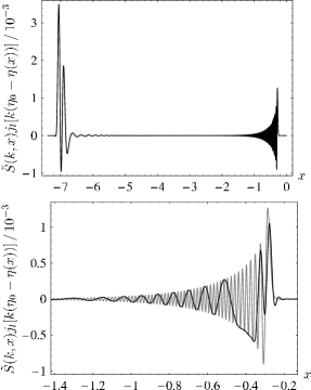
Figure 3: The integrand in (39) plotted as a function of $x$, for $l=100$ and $k=340H_{0}$. The top figure shows the entire integrand from last scattering until today, using the high resolution $x$- grid. The bottom figure shows a close-up where the oscillations in the Bessel function are important at late times, using the high resolution grid (gray line) and low resolution grid (black line). In both cases, we have used cubic splining between the actual samples of the integrand.

Amazingly, the CMB power spectrum calculated from the low and high resolution grids are indistinguishable. This is probably because the dominant part of the $x$-integration comes from recombination, with only a small correction from the late time oscillations caused by the Bessel function. The source function is non-zero at late times mostly due to the integrated Sachs-Wolfe effect, which is most important for low $l$’s ($\sim$ low $k$’s), whereas the oscillations in the Bessel function dominate for large $k$’s, hence the details of the oscillations are unimportant.

The spherical Bessel functions can be calculated using algorithms described in NumRec . The argument of the function should be chosen from 0 to $k_{\max}\eta_{0}\sim 3400$, and with 10 samples for each oscillation of width $2\pi$ we need about 5400 samples for each $l$ . The result is then splined to give a smooth function. The calculation takes a few seconds for each $l$, but since the Bessel functions are independent of the cosmological model, they can be calculated once and saved to disc for fast access later.

Finally, the actual integration across $x$ can be done using either a simple linear interpolation between the points from the (low or high resolution) grid, or using a more accurate cubic splining . Also in this case, the resulting CMB power spectrum is essentially the same, so we therefore choose the faster linear interpolation.

V.4 Integrating across $k$ and calculating $C_{l}$

The integrand in the final $k$-integration, (45), is an oscillating function of $k$. (This is why we needed the source function for more $k$’s than the ones where we actually integrated the differential equations.) Since the dominant contribution to the $x$-integration is from recombination where $\eta\ll\eta_{0}$, we have the rough estimate

$$\Theta_{l}(k)\sim j_{l}(k\eta_{0})\int_{0}^{\eta_{0}}S(k,\eta)d\eta\sim\mathrm{const}\cdot j_{l}(k\eta_{0})\,,$$ (53)

since the source function varies much slower with $k$ than the Bessel function. Thus,

$$C_{l}\sim\int_{0}^{\infty}\frac{j_{l}^{2}(k\eta_{0})}{k}dk\,.$$ (54)

The Bessel oscillations with period $2\pi$ means that the integrand has oscillations with period $\Delta k=2\pi/\eta_{0}$. In order to sample each oscillation with 10 points, we must therefore use a grid with resolution

$$\Delta k=\frac{2\pi}{10\eta_{0}}$$ (55)

for the $k$-integration. (This leads to the total number of $k$’s $(10\eta_{0}/2\pi)(k_{\max}-k_{\min})\sim 5000$ in section V.2.)

Figure 4: The integrand in (45) plotted as a function of $k$, for $l=100$. The peak is slightly after $k=l/\eta_{0}\simeq 29.4H_{0}$, and the integrand approaches zero very fast for smaller $k$. For larger $k$, however, the integrand dies out much more slowly, and even $k_{\max}/H_{0}\sim l$ is too small for an accurate calculation when $l=100$. With the adaptive algorithm described below, the integration continues all the way to $k=454.9H_{0}\sim 15\,l/\eta_{0}$.

The computation time can be reduced a bit by observing that the full range $0.1H_{0}\leq k\leq 1000H_{0}$ is not needed for all $l$. Instead, from (54) we see that the peak of the integrand is around $k\sim l/\eta_{0}$. The integrand falls of sharply for smaller $k$, but much more smoothly for larger $k$, as figure 4 shows. As a first estimate, we could try the integration range

$$\frac{0.9l}{\eta_{0}}\leq k\leq\frac{2l}{\eta_{0}}\,.$$ (56)

Using only this interval gives a rather inaccurate result, but we know that this interval at least contains the peak of the integrand. One possible algorithm is then to extend the interval in steps of one oscillation of width $\Delta k=2\pi/\eta_{0}$, both to the left and to the right of the initial interval, and compare the maximum value of the integrand within each step to the global maximum. We stop when the local maximum has been reduced to less than, say, $10^{-4}$ of the global. This algorithm gives a CMB power spectrum identical to using the full interval, but the $k$-integration runs about twice as fast, since on average we end up using only half of the interval.

Since we only do one $k$-integration for each $l$ (in contrast to several thousand $x$-integrations), we can use the slower but more accurate cubic splining instead of linear interpolation for the actual integration. The impact on the speed of the algorithm from this is negligible.

Finally, we don’t need to calculate $C_{l}$ explicitely for every $l$. Instead, since the CMB power spectrum is a rather smooth function of $l$, we only calculate $C_{l}$ for a few $l$’s and use cubic splining to get a smooth function . For low $l$’s we should use higher resolution. We choose the points $l=2$, 3, 4, 6, 8, 10, 12, 15 and 20, and then every 10th $l$ up to $l=100$, every 20th up to $l=200$, every 25th up to $l=300$, and finally every 50th $l$ above that. This gives a total of 44 $C_{l}$-calculations with $l_{\max}=1200$, and the entire integration (across both $x$ and $k$) only takes about 20 seconds with precalculated Bessel functions. Thus, the calculation of the CMB power spectrum is completed in about two and a half minutes.

V.5 Normalization

The final point that has to be considered conserns the normalization of the entire power spectrum. The power spectrum must be properly normalized if we want to compare it to CMBFAST. If we want to compare just one single model, we could simply use the height of e.g. the first peak as normalization. However, since this height depends on cosmological parameters, we must be more careful if we want to compare several different models within the same figure, like in figure 5, 6 and 7.

CMBFAST uses the COBE normalization Bunn_White , which basically normalizes to the observed spectrum from COBE. The idea is to use a least squares fit of the spectrum for $l\leq 20$  (since COBE is only accurate on this scale) to a quadratic function in $x\equiv\log_{10}l$:

$$l(l+1)C_{l}\simeq D_{1}\!\left[1+D^{\prime}(x-1)+D^{\prime\prime}(x-1)^{2}/2\right].$$ (57)

From their definition $D^{\prime}$ and $D^{\prime\prime}$ are independent of normalization, and parametrize the shape of the spectrum. The fit to the COBE data is then given approximately by the formula Bunn_White

$$10^{11}C_{10} = 0.64575+0.02282D^{\prime}+0.01391(D^{\prime})^{2}$$

$$-0.01819D^{\prime\prime}\!-\!0.00646D^{\prime}D^{\prime\prime}\!+\!0.00103(D^{\prime\prime})^{2},$$

i.e. the value of $C_{10}$ is fixed by this expression, and the normalization of the rest of the spectrum then follows by multiplying the calculated $C_{l}$’s by the appropriate constant. One should be aware that this normalization may actually introduce a quite significant uncertainty when comparing the spectrum to CMBFAST. Part of the reason is that inaccuracies in the calculation of the low $l$’s get transferred to the entire spectrum by this method. By fine-tuning the normalization, the relative error in the plots of section VI can be reduced by up to a factor of 2. Since in practice what one really want is to fit the calculated spectrum to observational data, and not to CMBFAST or some other program, one should probably start using the entire spectrum in the normalization instead of the COBE normalization. Also note that CMBFAST gives its output as $l(l+1)C_{l}/2\pi$, where the factor $2\pi$ is the commonly used convention.

VI Results

Here we compare our program to CMBFAST for some cosmological models. In figure 5 we vary the Hubble constant $h$ between $0.66$ and $0.74$, in figure 6 we vary the baryon density $\Omega_{b}$ between $0.042$ and $0.050$, in figure 7 we vary the CDM density $\Omega_{m}$ between $0.200$ and $0.248$, and in figure 8 we vary the spectral index $n$ between $0.95$ and $1$. In figure 9 we also plot the power spectrum up to $l=2000$ for the default model. Following this is the spectrum with helium included (figure 10, section VII.1), a simple model of reionization (figure 11, section VII.2), massless neutrinos (figure 12, section VII.3), and finally the polarization and temperature – polarization cross correlation power spectrum (figures 13 and 14, section VII.4).

Figure 5: Our program compared to CMBFAST when varying the Hubble constant: the default model $h=0.70$ (solid line), $h=0.66$ (dashed line), and $h=0.74$ (dotted line). The figure to the left shows our calculated power spectrum, and the figure to the right shows the relative error when compared to CMBFAST (C.F.), which we see is of order $0.3\,\%$ or below for most $l$’s. Because the error is so small, there’s no point in plotting the spectrum from CMBFAST in the figure to the left, since the difference between the curves would be smaller than the width of the lines.

Figure 6: Our program compared to CMBFAST when varying the baryon density: the default model $\Omega_{b}=0.046$ (solid line), $\Omega_{b}=0.042$ (dashed line), and $\Omega_{b}=0.050$ (dotted line). The relative error is still between $\sim 0.1\,\%$ and $0.3\,\%$.

Figure 7: Our program compared to CMBFAST when varying the CDM density: the default model $\Omega_{m}=0.224$ (solid line), $\Omega_{m}=0.200$ (dashed line), and $\Omega_{m}=0.248$ (dotted line).

Figure 8: Our program compared to CMBFAST when varying the spectral index: the default model $n=1$ (solid line), $n=0.975$ (dashed line), and $n=0.95$ (dotted line).

Figure 9: The power spectrum for the default model up to $l=2000$, compared to CMBFAST. The relative error starts to increase systematically beyond $l\sim 1000$. In this calculation we have used $k_{\max}=1500H_{0}$, with 150 values of $k$ chosen initially. We have also used $l_{\max}=8$ instead of $6$ in the Boltzmann hierarchy, which reduced the error for $l\sim 1800$ from $0.9\,\%$ down to about $0.65\,\%$.

Figure 10: The power spectrum with helium included (section VII.1), compared to CMBFAST: $Y_{p}=0$ (solid line), $Y_{p}=0.24$ (dashed line), and $Y_{p}=0.48$ (dotted line). The other cosmological parameters are as in the default model.

Figure 11: The power spectrum with reionization (section VII.2): $z_{ri}=5$ and $\Delta z=0.075$ (dashed line), $z_{ri}=10$ and $\Delta z=0.2$ (dotted line), and no reionization (solid line). We include helium ($Y_{p}=0.24$), otherwise the cosmological parameters are as in the default model.

Figure 12: The power spectrum with massless neutrinos included (section VII.3): $N_{\nu}=3$ (solid line), $N_{\nu}=1$ (dotted line), and $N_{\nu}=0$, i.e. without neutrinos (dashed line). Apart from the neutrinos the default model is used.

Figure 13: The E-mode polarization power spectrum (section VII.4) compared to CMBFAST for the default model (solid line), $n=0.95$ (dashed line), and $h=0.66$ (dotted line). The expression for the relative error is slightly modified so it doesn’t diverge when $C_{E,l}\to 0$: $\mathrm{Error}\equiv|C_{E,l}-C_{E,l}^{{}_{\mathrm{C.F.}}}|\,/\,(C_{E,l}^{{}_{\mathrm{C.F.}}}\!+\epsilon)$, where $l(l+1)\epsilon/2\pi=10^{-14}$. The large error of about $3\,\%$ close to $l=200$ is probably due to a slightly wrong position of the minimum. However, the value of $C_{E,l}$ is still very small here, and the relative error doesn’t really have a significant meaning until $l\gtrsim 300$.

Figure 14: The temperature – polarization cross correlation power spectrum compared to CMBFAST for the default model (solid line), $n=0.95$ (dashed line), and $h=0.66$ (dotted line). Since the relative difference is not very useful for a function that crosses zero several times, the figure to the right shows the absolute difference $\Delta_{C,l}\equiv C_{C,l}-C_{C,l}^{{}_{\mathrm{C.F.}}}$ instead. Note that, with the exception of a single point, our program always gives a larger value of $C_{C,l}$ than CMBFAST. This can not be due to wrong normalization, however, since $C_{C,l}$ is both positive and negative.

VII Including more ingredients

VII.1 Helium

The primordial mass fraction of ${}^{4}\mathrm{He}$, $Y_{p}$, is defined as the ratio between the total mass of helium and the total baryon mass. We define a ”baryon” as a proton or a neutron with a mass $m_{b}\simeq m_{\mathrm{H}}$. Each helium atom thus contains 4 baryons, and has a mass approximately equal to $4m_{\mathrm{H}}$, which gives Trotta_Hansen

$$Y_{p} \equiv \frac{M_{\mathrm{He}}}{M_{b}}\simeq\frac{n_{\mathrm{He}}m_{\mathrm{He}}}{n_{b}m_{\mathrm{H}}}\simeq\frac{4n_{\mathrm{He}}}{n_{b}}\,,$$

$$\frac{n_{\mathrm{H}}}{n_{b}} = \frac{n_{b}-4n_{\mathrm{He}}}{n_{b}}\simeq 1-Y_{p}\,.$$ (59)

Because of the larger ionization energy, helium recombines before hydrogen, so that during hydrogen recombination all helium is essentially neutral. The main effect of including helium is therefore that the number of free electrons during hydrogen recombination is reduced (when keeping $\Omega_{b}$ fixed). The recombination history of helium is well described by the Saha equation. Defining

$$x_{1}\equiv\frac{n_{\mathrm{He}^{+}}}{n_{\mathrm{He}}}\,,\qquad x_{2}\equiv\frac{n_{\mathrm{He}^{++}}}{n_{\mathrm{He}}}\,,\qquad x_{\mathrm{H}}\equiv\frac{n_{\mathrm{H}^{+}}}{n_{\mathrm{H}}}\,,$$ (60)

we now have three Saha equations Ma_Bert

$$n_{e}\frac{x_{1}}{1-x_{1}-x_{2}} = 2\left(\frac{m_{e}T_{b}}{2\pi}\right)^{3/2}e^{-\chi_{0}/T_{b}}\,,$$

$$n_{e}\frac{x_{2}}{x_{1}} = 4\left(\frac{m_{e}T_{b}}{2\pi}\right)^{3/2}e^{-\chi_{1}/T_{b}}\,,$$

$$n_{e}\frac{x_{\mathrm{H}}}{1-x_{\mathrm{H}}} = \left(\frac{m_{e}T_{b}}{2\pi}\right)^{3/2}e^{-\epsilon_{0}/T_{b}}\,,$$ (61)

instead of the one in (12). They are linked in a non-trivial way, because the number density of free electrons is now

$$n_{e} = 2n_{\mathrm{He}^{++}}+n_{\mathrm{He}^{+}}+n_{\mathrm{H}^{+}}$$ (62)

$$= \left[\raisebox{0.0pt}[5.69054pt][5.69054pt]{$\displaystyle(2x_{2}+x_{1})Y_{p}/4+x_{\mathrm{H}}(1-Y_{p})$}\right]n_{b}\equiv f_{e}n_{b}\,.\hskip 17.07164pt$$

The ionization energy of neutral and singly ionized helium is

$$\chi_{0}=24.5874\;\mathrm{eV}\,,\qquad\chi_{1}=4\,\epsilon_{0}=54.42279\;\mathrm{eV}\,.$$ (63)

Eqs. (61) and (62) are most easily solved by noting that they will only be used before hydrogen recombination becomes important, thus $f_{e}$ is of order 1 the whole time . We therefore use (61) to express $x_{1}$, $x_{2}$ and $x_{\mathrm{H}}$ in terms of $f_{e}$, and then use (62) recursively with $f_{e}=1$ as a starting value. The full machine precision of 15 digits is then reached in less than 10 steps. Finally, the electron fraction $X_{e}$ defined in (10) is given by

$$X_{e}\equiv\frac{n_{e}}{n_{\mathrm{H}}}=\frac{f_{e}}{1-Y_{p}}\,.$$ (64)

We switch to the more accurate Peebles equation once hydrogen recombination starts fully ($X_{e}<0.99$). At this point all helium is neutral, and the only difference from section II.2 is that the hydrogen density is now smaller than the baryon density. That is, the only changes to eqs. (13) and (14) are

$$\frac{dX_{e}}{dx} = \frac{C_{r}(T_{b})}{H}\!\left[\beta(T_{b})(1\!-\!X_{e})-(1\!-\!Y_{p})n_{b}\alpha^{(2)}(T_{b})X_{e}^{2}\right]\!,$$

$$n_{1s} = (1-X_{e})(1-Y_{p})\,n_{b}\,,$$ (65)

i.e. $n_{\mathrm{H}}$ is replaced by $(1-Y_{p})n_{b}$ everywhere. The resulting solution $X_{e}$ is shown in figure 15 for $Y_{p}=0.24$. Note that $X_{e}>1$ before helium recombination.

Figure 15: The electron fraction $X_{e}$ with helium mass fraction $Y_{p}=0.24$ (solid line) as a function of redshift, compared to $Y_{p}=0$ (dashed line). The first helium recombination $\mathrm{He}^{++}\to\mathrm{He}^{+}$ occurs around $z\sim 6000$, and the second $\mathrm{He}^{+}\to\mathrm{He}$ around $z\sim 2500$. For $z\gtrsim 6000$ when helium is doubly ionized $X_{e}\simeq(1-Y_{p}/2)/(1-Y_{p})=1.1579$, and for $2500\lesssim z\lesssim 6000$ when helium is singly ionized $X_{e}\simeq(1-3Y_{p}/4)/(1-Y_{p})=1.0789$. The residual electron fraction at late times is larger by a factor $1/(1-Y_{p})$ with helium included.

Once the free electron density and the resulting optical depth have been calculated, the rest of the CMB calculation proceeds exactly as without helium. In figure 10 we compare our program to CMBFAST for $Y_{p}=0$, $Y_{p}=0.24$ and $Y_{p}=0.48$ (and the other parameters as in the default model). The precision with helium included is just as good as without. One should also note that the other elements (D, ${}^{3}\mathrm{He}$, Li etc.) only give corrections to the CMB power spectrum of order $10^{-5}$ Hu_Scott .

VII.2 Reionization

At some time long after recombination, we know that the hydrogen in the universe became more of less fully ionized again. This was probably the result of the energetic radiation from the first generation of stars, with enough energy to ionize hydrogen, but too low energy to ionize helium, which therefore remained neutral. The detailed mechanism of this process is not fully understood, but one possible model is to simply assume that at a certain redshift $z_{ri}$ the free electron fraction $X_{e}$ instantly jumps to a constant value, usually $X_{e}=1$, and then stays there until today.

With instant reionization, both the optical depth $\tau^{\prime}$ and the visibility function $\tilde{g}$ experience a jump discontinuity at $z=z_{ri}$, and thus a delta function in $\tilde{g}^{\prime}$. This can be a bit tricky to implement directly in our program, and since it is not very physical either, it is probably better to use a smooth (but still sharp) transition from the Peebles result to $X_{e}=1$ around $z_{ri}$. We choose the simple formula 

$$X_{e}(z) = X^{\mathrm{Peebles}}_{e}(z)\cdot(1-f)+1\cdot f\,,$$

$$f(z) = \frac{1}{\pi}\arctan\left[\frac{10(z_{ri}-z)}{\Delta z}\right]+\frac{1}{2}\,,$$ (66)

where $\Delta z$ can be interpreted as the width of the reionization period, typically chosen to be of order $0.2$. Figure 16 shows the free electron fraction, optical depth and visibility function with $z_{ri}=10$ and $\Delta z=0.2$.

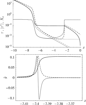
Figure 16: The top figure shows the optical depth $\tau$ (solid line) and $|\tau^{\prime}|$ (dashed line), and the free electron fraction $X_{e}$ (dotted line), as functions of $x$. The black lines show the semi-instant reionization of eq. (66) with $z_{ri}=10$ and $\Delta z=0.2$, and the gray lines are without reionization, both for the default model with helium ($Y_{p}=0.24$). The plateau $\tau(z>z_{ri})\simeq 0.075$ is the optical depth to the last scattering surface. The bottom figure shows the visibility function $\tilde{g}=-\tau^{\prime}e^{-\tau}$ (solid line), its derivative $\tilde{g}^{\prime}/180$ (dashed line), and its double derivative $\tilde{g}^{\prime\prime}/65\,000$ (dotted line).

Because of the sharp peak in $\tilde{g}^{\prime}$, we must use higher resolution for the grid of $x$-values near reionization when calculating the source function. We choose to use an additional 200 points between $z_{ri}+\Delta z$ and $z_{ri}-\Delta z$, evenly distributed in $x$. The rest of the calculation then proceeds as without reionization. The resulting CMB power spectrum agrees very well with CMBFAST, even if CMBFAST uses truly instant reionization. We should choose $\Delta z$ as small as possible to simulate instant reionization. Choosing $\Delta z$ too small, however, leads to problems, since the $x$-grid must then have an even higher resolution, possibly also outside the interval $\left[z_{ri}+\Delta z\,,\,z_{ri}-\Delta z\right]$. We get the best agreement with CMBFAST when $\Delta z=0.2$ for $z_{ri}=10$, and $\Delta z=0.075$ for $z_{ri}=5$. Figure 11 shows the power spectrum compared to CMBFAST.

VII.3 Massless neutrinos

The neutrinos decoupled from the cosmic plasma slightly before the annihilation of electrons and positrons, when the temperature was of order the electron mass. The photons were heated by this process, so the neutrino temperature is therefore lower by a factor Dodelson

$$\frac{T_{\nu}}{T_{r}}=\left(\frac{4}{11}\right)^{1/3}\simeq 0.714\,.$$ (67)

The ratio between the energy densities of neutrinos and photons is thus 

$$\frac{\rho_{\nu}}{\rho_{r}}=\frac{\Omega_{\nu}}{\Omega_{r}}=N_{\nu}\cdot\frac{7}{8}\!\left(\!\frac{4}{11}\!\right)^{\!4/3}\!\!\!\simeq 0.681\,,\quad(\mathrm{for}\;N_{\nu}=3)\,,$$ (68)

where $N_{\nu}$ is the number of neutrino species, and the factor $7/8$ is because neutrinos are fermions. Actually, since neutrinos are not completely decoupled when the cosmic plasma is reheated, one should use an effective number of neutrinos $N_{\nu}=3.04$ Lopez . With neutrinos as a new component, the Hubble function (2) is of course modified. The cosmological constant $\Omega_{\Lambda}$ in (16) is also slightly reduced if $\Omega_{b}$ and $\Omega_{m}$ are fixed.

The initial conditions for the neutrino monopole and dipole are the same as for photons:

$${\cal N}_{0} = \Theta_{0}=\frac{1}{2}\Phi\,,$$

$${\cal N}_{1} = \Theta_{1}=-\frac{k}{6{\cal H}}\Phi\,.$$ (69)

The quadropole is more complicated. Since $\Theta_{2}\ll{\cal N}_{2}$, the gravitational potentials are initially related by Dodelson

$$\Phi = -\Psi\left(1+\frac{2f_{\nu}}{5}\right),$$ (70)

$$f_{\nu} \equiv \frac{\rho_{\nu}}{\rho_{r}\!+\!\rho_{\nu}}=\frac{1}{\frac{8}{7N_{\nu}\!}\!\left(\frac{11}{4}\right)^{4/3}\!+\!1}\simeq 0.405\,,\quad(\mathrm{for}\;N_{\nu}=3)\,.$$

From (22) this gives the initial value

$${\cal N}_{2}=-\frac{k^{2}a^{2}\Phi}{12H_{0}^{2}\Omega_{\nu}}\frac{1}{\frac{5}{2f_{\nu}}+1}\,.$$ (71)

Note that ${\cal N}_{2}\sim a^{2}$ at early times. For the higher multipoles we can assume that ${\cal N}_{l}\ll{\cal N}_{l-1}$. Using (71) and ${\cal H}\simeq H_{0}\sqrt{\Omega_{r}+\Omega_{\nu}}\,a^{-1}$ in (22) then gives a differential equation for ${\cal N}_{3}$ that can be integrated directly, with the result that ${\cal N}_{3}\sim a^{3}$. Continuing this way we get ${\cal N}_{l}\sim a^{l}$, meaning that ${\cal N}^{\prime}_{l}\simeq l{\cal N}_{l}$, and therefore

$${\cal N}_{l}\simeq\frac{k}{(2l+1){\cal H}}{\cal N}_{l-1}\,,\qquad l\geq 3\,,$$ (72)

as the initial condition for the higher multipoles. Finally, we use the same cutoff scheme for the neutrino hierarchy as for the photons,

$${\cal N}^{\prime}_{l}\simeq\frac{k}{{\cal H}}{\cal N}_{l-1}-\frac{l+1}{{\cal H}\eta(x)}{\cal N}_{l}\,,\qquad l=l_{\max}\,.$$ (73)

We choose $l_{\max}=10$ for the neutrino multipoles in order to get sufficient precision for large $l$’s. Note that ${\cal H}\eta\simeq 1$ at early times, so that (73) reduces to ${\cal N}^{\prime}_{l}\simeq l{\cal N}_{l}$ directly when using (72).

As a curiosity we find that

$$\lim_{N_{\nu}\to 0}{\cal N}_{2}^{\mathrm{init}}=-\frac{k^{2}a^{2}\Phi}{30H_{0}^{2}\Omega_{r}}\,.$$ (74)

All the equations where neutrinos appear are therefore well-defined in the limit $N_{\nu}\to 0$. The hierarchy of neutrino multipoles is still non-vanishing in this limit, but the neutrinos no longer contribute to the CMB power spectrum since they decouple from the gravitational potential. The result is therefore the same as if the neutrino hierarchy had not been included at all, as expected.

The rest of the CMB calculation is exactly the same as without neutrinos, as long as one uses the correct expression for $\Psi$ in the source function (40). Figure 12 shows the power spectrum for $N_{\nu}=3$, $1$ and $0$ compared to CMBFAST. The agreement is very good below $l\sim 600$, but the error increases somewhat faster for large $l$’s than without neutrinos.

VII.4 Polarization power spectrum

So far, we have only considered the temperature power spectrum of the CMB. However, since the radiation is polarized, we also have both a polarization power spectrum and a cross correlation power spectrum between temperature and polarization. With the recent release of the three-year results of WMAP WMAP_threeyear , these spectra will be of great interest since we now have measurements of the full sky CMB polarization map.

A radiation field in general needs four parameters to be described completely, called the Stokes parameters. These are the temperature $T$, linear polarization $Q$ and $U$ along two different directions, and circular polarization $V$. $T$ and $V$ are rotationally invariant and can therefore be expanded in spherical harmonics . $Q$ and $U$, on the other hand, transform under rotations in the plane perpendicular to the direction of the photons. It turns out that the linear combination $Q\pm iU$ transforms in a particularly simple way. Under a rotation $\psi$ it transforms as $(Q\pm iU)^{\prime}=e^{\mp 2i\psi}(Q\pm iU)$, i.e. it has spin $\pm 2$ and can therefore be expanded in what is called spin $\pm 2$ spherical harmonics  (see Zald_Seljak for more details). It also means that we can define spin zero quantities by acting on $Q\pm iU$ twice using the spin raising operator $\eth$ or the spin lowering operator $\overline{\eth}$ (again see Zald_Seljak for the details)

$$\tilde{E}(\mu) \equiv -\frac{1}{2}\left[\raisebox{0.0pt}[5.69054pt][5.69054pt]{$\displaystyle\overline{\eth}{}^{\>\!2}(Q+iU)+\eth^{2}(Q-iU)$}\right],$$

$$\tilde{B}(\mu) \equiv \frac{i}{2}\left[\raisebox{0.0pt}[5.69054pt][5.69054pt]{$\displaystyle\overline{\eth}{}^{\>\!2}(Q+iU)-\eth^{2}(Q-iU)$}\right].$$ (75)

The power spectra for $\tilde{E}$ and $\tilde{B}$ are thus rotationally invariant, and can be used to describe the polarization of the CMB radiation.

When we are only considering scalar perturbations, we can choose a coordinate system (for each Fourier mode) where $U=0$. We then have $Q=\Theta_{P}$ and $\overline{\eth}{}^{\>\!2}Q=\eth^{2}Q$ since $\Theta_{P}$ only depends on the polar angle. Thus we only get E-mode polarization from scalar perturbations. (Tensor perturbations generate both E- and B-mode polarization.) We use the line-of-sight integration method for polarization, similar to the temperature, and get from (20)

$$\Theta_{P}(k,\mu,\eta_{0}) = -\frac{1}{2}\int_{0}^{\eta_{0}}\dot{\tau}(1-{\cal P}_{2})\Pi e^{ik\mu(\eta-\eta_{0})-\tau}d\eta$$ (76)

$$= \frac{3}{4}\int_{0}^{\eta_{0}}g\Pi(1-\mu^{2})e^{ik\mu(\eta-\eta_{0})}d\eta\,.$$

This gives Zald_Seljak

$$\tilde{E}(k,\mu,\eta_{0}) = -\frac{3}{4}\int_{0}^{\eta_{0}}g\Pi\partial_{\mu}^{2}\left[(1-\mu^{2})^{2}e^{-i\mu x}\right]\!d\eta$$ (77)

$$= \frac{3}{4}\int_{0}^{\eta_{0}}g\Pi(1+\partial_{x}^{2})^{2}(x^{2}e^{-i\mu x})\,d\eta\,,$$

where $x=k(\eta_{0}-\eta)$. Expanding in multipoles, we get 

$$\Theta^{E}_{l}(k,\eta_{0}) = \frac{3}{4}\sqrt{\frac{(l-2)!}{(l+2)!}}\int_{0}^{\eta_{0}}g\Pi(1+\partial_{x}^{2})^{2}\!\left[x^{2}j_{l}(x)\right]\!d\eta$$

$$= \frac{3}{4}\sqrt{\frac{(l+2)!}{(l-2)!}}\int_{0}^{\eta_{0}}g\Pi\frac{j_{l}(x)}{x^{2}}d\eta$$

$$= \sqrt{\frac{(l+2)!}{(l-2)!}}\int_{0}^{\eta_{0}}S_{E}(k,\eta)j_{l}[k(\eta_{0}-\eta)]d\eta\,,$$

$$S_{E}(k,\eta) = \frac{3g\Pi}{4k^{2}(\eta_{0}-\eta)^{2}}\,.$$ (78)

Here we have used the result $(1+\partial_{x}^{2})^{2}\!\left[x^{2}j_{l}(x)\right]\!=(l-1)l(l+1)(l+2)j_{l}(x)/x^{2}$, which follows from the differential equation $j^{\prime\prime}_{l}+2j^{\prime}_{l}/x+\!\left[1-l(l+1)/x^{2}\right]\!j_{l}=0$ satisfied by the spherical Bessel function. The E-mode polarization power spectrum and its cross correlation with temperature is then finally given by Zald_Seljak

$$C_{E,l} = \int_{0}^{\infty}\left(\frac{k}{H_{0}}\right)^{n-1}\Theta_{El}^{2}(k)\frac{dk}{k}\,,$$

$$C_{C,l} = \int_{0}^{\infty}\left(\frac{k}{H_{0}}\right)^{n-1}\Theta_{l}(k)\Theta^{E}_{l}(k)\frac{dk}{k}\,.$$ (79)

Figure 13 shows the E-mode polarization and figure 14 the temperature – polarization cross correlation compared to CMBFAST for a few models. The calculation uses exactly the same algorithms and techniques as for the temperature, only with $l_{\max}=8$ instead of $6$ in the Boltzmann hierarchy to get acceptable precision for the polarization multipoles.

VIII Conclusion

We have here presented all the main steps required in writing a program that calculates the CMB anisotropy power spectrum. Our focus has been on the computer-technical side of the problem, by including all the small details that make the program actually work, something which is often left out in the literature. We have consentrated on the $\Lambda\mathrm{CDM}$ model, where the program achieves an accuracy comparable to CMBFAST  ($\sim\,0.1\,\%$ – $0.4\,\%$) over a range of cosmological parameters. The program runs in a couple of minutes on a mid-range personal computer (as of 2006). While certainly not as good as CMBFAST, this is still acceptable considering that the code hasn’t really been optimized for speed.

The purpose of this work has been to give a running start to those needing to calculate the CMB power spectrum for some exotic cosmological model where the standard programs can’t be used. With the growing precision of the observed spectrum, a calculation to within the $1\,\%$ level is often what distinguishes the models and makes it possible to rule out some of them. We hope this work will encourage others by showing that writing a program from scratch to within this accuracy is not really as difficult or time-consuming as one may think.

Acknowledgement: I want to thank Tomi Koivisto for very useful discussions about the various programming techniques involved in writing the program. This work has been supported by grant no. NFR 153577/432 from the Research Council of Norway.

References

- (1) G. F. Smoot et al., Astrophys. J. Lett. 396, L1 (1992)
- (2) C. L. Bennett et al., Astrophys. J. Suppl. 148, 1 (2003), astro-ph/0302207; D. N. Spergel et al., Astrophys. J. Suppl. 148, 175 (2003), astro-ph/0302209
- (3) D. N. Spergel et al., astro-ph/0603449; L. Page et al., astro-ph/0603450; G. Hinshaw et al., astro-ph/0603451; N. Jarosik et al., astro-ph/0603452
-
(4)
See the Planck satellite webpage at
http://www.rssd.esa.int/index.php?project=planck or http://www.esa.int/science/planck - (5) D. Scott, astro-ph/0510731
-
(6)
The CMBFAST program package is written by U. Seljak and M. Zaldarriaga. See
its webpage at
http://www.cmbfast.org -
(7)
A web interface of CMBFAST can be found at
http://lambda.gsfc.nasa.gov/cgi-bin/cmbfast_form.pl. All spectra from CMBFAST in this text have been obtained from this web form. - (8) M. Doran, JCAP 0510, 011 (2005), astro-ph/0302138; See also its webpage http://www.cmbeasy.org
- (9) A. Lewis, A. Challinor and A. Lasenby, Astrophys. J. 538, 473 (2000), astro-ph/9911177; See also its webpage http://camb.info
- (10) http://www.borland.com/delphi
- (11) S. Dodelson, Modern cosmology, Academic Press (2003)
- (12) C.-P. Ma and E. Bertschinger, Astrophys. J. 455, 7 (1995), astro-ph/9506072
- (13) W. Hu, Annals Phys. 303, 203 (2003), astro-ph/0210696
- (14) R. Keskitalo, Master thesis, University of Helsinki, Helsinki (2005)
- (15) M. Doran, JCAP 0506, 011 (2005), astro-ph/0503277
- (16) M. Zaldarriaga and D. D. Harari, Phys. Rev. D52, 3276 (1995), astro-ph/9504085
- (17) U. Seljak and M. Zaldarriaga, Astrophys. J. 469, 437 (1996), astro-ph/9603033
- (18) W. H. Press, S. A. Teukolsky, W. T. Vetterling and B. P. Flannery, Numerical Recipes in C, Cambridge University Press (2002)
- (19) E. F. Bunn and M. White, Astrophys. J. 480, 6 (1997), astro-ph/9607060
- (20) R. Trotta and S. H. Hansen, Phys. Rev. D69, 023509 (2004), astro-ph/0306588
- (21) W. Hu, D. Scott, N. Sugiyama and M. White, Phys. Rev. D52, 5498 (1995), astro-ph/9505043
- (22) R. E. Lopez, S. Dodelson, A. Heckler and M. S. Turner, Phys. Rev. Lett. 82, 3952 (1999), astro-ph/9803095
- (23) M. Zaldarriaga and U. Seljak, Phys. Rev. D55, 1830 (1997), astro-ph/9609170
- (24) M. Kamionkowski, A. Kosowsky and A. Stebbins, Phys. Rev. D55, 7368 (1997), astro-ph/9611125
- (25) U. Seljak, N. Sugiyama, M. White and M. Zaldarriaga, Phys. Rev. D68, 083507 (2003), astro-ph/0306052