Mass Accretion onto T Tauri Stars

Abstract

It is now accepted that accretion onto classical T Tauri stars is controlled by the stellar magnetosphere, yet to date most accretion models have assumed that their magnetic fields are dipolar. By considering a simple steady state accretion model with both dipolar and complex magnetic fields we find a correlation between mass accretion rate and stellar mass of the form $\dot{M}\propto M_{\ast}^{\alpha}$, with our results consistent within observed scatter. For any particular stellar mass there can be several orders of magnitude difference in the mass accretion rate, with accretion filling factors of a few percent. We demonstrate that the field geometry has a significant effect in controlling the location and distribution of hot spots, formed on the stellar surface from the high velocity impact of accreting material. We find that hot spots are often at mid to low latitudes, in contrast to what is expected for accretion to dipolar fields, and that particularly for higher mass stars, the accretion flow is predominantly carried by open field lines.

1 Introduction

Classical T Tauri stars (CTTSs) are young, low mass, pre-main sequence stars that are actively accreting from a surrounding disc which is the eventual birth-place of planets. Uchida & Shibata (1984) suggested that the magnetic field of a CTTS disrupts the inner disc. In the early 1990s several magnetospheric accretion models were developed (Königl 1991; Collier Cameron & Campbell 1993; Shu et al. 1994) where material is lifted from the disc plane and is channelled along dipolar magnetic field lines onto the star, terminating in a shock at the photosphere. In an idealised model of a CTTS’s magnetic field there are closed field lines close to the star that contain the X-ray emitting corona, whilst at larger radii, there are closed field lines which thread the circumstellar disc. It is along this latter set of field lines that accretion may proceed. There are also regions of open field which carry outflows in the form of a wind, and in some cases, as large collimated bipolar jets.

Magnetospheric accretion models assume that CTTSs possess magnetic fields that are strong enough to disrupt the disc at a distance of a few stellar radii. Such strong fields have been detected in a number of systems using a variety of techniques. Average surface fields of 1-3kG have been detected most successfully by exploiting the Zeeman effect, both through Zeeman broadening (e.g. Johns-Krull, Valenti & Koresko 1999b) and from the circular polarisation of lines which are sensitive to the presence of a magnetic field (e.g. Johns-Krull et al. 1999a; Symington et al. 2005; Daou, Johns-Krull & Valenti 2006). Field detections have also been made from the increase in line equivalent width (Basri, Marcy & Valenti 1992; Guenther et al. 1999) and also from electron cyclotron maser emission, a coherent emission process from mildly relativistic electrons trapped inside flux tubes close to the star (Smith et al., 2003). The mean magnetic field strengths detected so far appear to be roughly constant across all stars (Valenti & Johns-Krull, 2004).

Traditionally magnetospheric accretion models have assumed the CTTSs have dipolar magnetic fields. Dipole fields (or inclined dipole fields) have been successively used to explain some of the observations of CTTSs (e.g. the photopolarimetric variability of AA Tau, O’Sullivan et al. 2005), but fail to account for others. Valenti & Johns-Krull (2004) present magnetic field measurements for a number of stars, and despite detecting strong average surface fields from Zeeman broadening, often measurements of the longitudinal (line-of-sight) field component (obtained from photospheric lines) are consistent with no net circular polarisation. This can be interpreted as there being many regions of opposite polarity on the stellar surface, giving rise to oppositely polarised signals which cancel each other out giving a net polarisation signal of zero. This suggests that CTTSs have magnetic fields which are highly complex, particularly close to the stellar surface; however, as Valenti & Johns-Krull (2004) point out, as the higher order multi-pole field components will drop off quickly with distance from the star, the dipole component may still remain dominant at the inner edge of the disc. Also their measurements of the circular polarisation of the HeI 5876Å emission line (believed to form in the base of accretion columns) are well fitted by a simple model of a single magnetic spot on the surface of the star, suggesting that the accreting field may be well ordered, despite the surface field being complex.

The fractional surface area of a CTTS which is covered in hot spots, the accretion filling factor $f_{acc}$, is inferred from observations to be small; typically of order one percent (Muzerolle et al. 2003; Calvet et al. 2004; Valenti & Johns-Krull 2004; Symington et al. 2005; Muzerolle et al. 2005). Dipolar magnetic field models predict accretion filling factors which are too large. This, combined with the polarisation results, led Johns-Krull & Gafford (2002) to generalise the Shu X-wind model (Shu et al., 1994) to include multipolar, rather than dipolar, magnetic fields. With the assumption that the average surface field strength does not vary much from star to star the generalised Shu X-wind model predicts a correlation between the stellar and accretion parameters of the form $R_{\ast}^{2}f_{acc}\propto(M_{\ast}\dot{M}P_{rot})^{1/2}$, a prediction that matches observations reasonably well.

In this paper we present a model of the accretion process using both dipolar and complex magnetic fields. We apply our model to a large sample of pre-main sequence stars obtained from the Chandra Orion Ultradeep Project (COUP; Getman et al. 2005), in order to test if our model can reproduce the observed correlation between mass accretion rate and stellar mass. An increase in $\dot{M}$ with $M_{\ast}$ was originally noted by Rebull et al. (2000) and subsequently by White & Ghez (2001) and Rebull et al. (2002). The correlation was then found to extend to very low mass objects and accreting brown dwarfs by White & Basri (2003) and Muzerolle et al. (2003), and to the higher mass, intermediate mass T Tauri stars, by Calvet et al. (2004). Further low mass data has recently been added by Natta et al. (2004), Mohanty, Jayawardhana & Basri (2005) and by Muzerolle et al. (2005) who obtain a correlation of the form $\dot{M}\propto M_{\ast}^{2.1}$, with as much as three orders of magnitude scatter in the measured mass accretion rate at any particular stellar mass. However, Calvet et al. (2004) point out that due to a bias against the detection of higher mass stars with lower mass accretion rates, the power may be less than 2.1. Further data for accreting stars in the $\rho-$Ophiuchus star forming region has recently been added by Natta, Testi & Randich (2006).

The physical origin of the correlation between $M_{\ast}$ and $\dot{M}$, and the large scatter in measured $\dot{M}$ values, is not clear; however several ideas have been put forward. First, increased X-ray emission in higher mass T Tauri stars (Preibisch et al. 2005; Jardine et al. 2006) may cause an increase in disc ionisation, leading to a more efficient magnetorotational instability and therefore a higher mass accretion rate (Calvet et al., 2004). Second, Padoan et al. (2005) argue that the correlation $\dot{M}\propto M_{\ast}^{2}$ arises from Bondi-Hoyle accretion, with the star-disc system gathering mass as it moves through the parent cloud. In their model the observed scatter in $\dot{M}$ arises from variations in stellar velocities, gas densities and sound speeds. Mohanty et al. (2005) provide a detailed discussion of both of these suggestions. Third, Alexander & Armitage (2006) suggest that the correlation may arise from variations in the disc initial conditions combined with the resulting viscous evolution of the disc. In their model they assume that the initial disc mass scales linearly with the stellar mass, $M_{d}\propto M_{\ast}$, which, upon making this assumption, eventually leads them to the conclusion that brown dwarfs (the lowest mass accretors) should have discs which are larger than higher mass accretors. However, if it is the case that the initial disc mass increases more steeply with stellar mass, $M_{d}\propto M_{\ast}^{2}$, then the stellar mass - accretion rate correlation can be reproduced with smaller brown dwarf discs of low mass (of order one Jupiter mass). Thus the Alexander & Armitage (2006) suggestion, if correct, will soon be directly verifiable by observations. Fourth, Natta et al. (2006) suggest that the large scatter in the correlation between $\dot{M}$ and $M_{\ast}$ may arise from the influence of close companion stars, or by time variable accretion. It should however be noted that Clarke & Pringle (2006) take a more conservative view by demonstrating that a steep correlation between $\dot{M}$ and $M_{\ast}$ may arise as a consequence of detection/selection limitations, and as such $\dot{M}\propto M_{\ast}^{2}$ is perhaps not a true representation of the correlation between $\dot{M}$ and $M_{\ast}$.

In §2 we describe how magnetic fields are extrapolated from observed surface magnetograms. In §3 we consider accretion onto an aligned, and then a tilted dipole field, to develop a simple steady state accretion model and to investigate how tilting the field affects the mass accretion rate. In §4 these ideas are extended by considering magnetic fields with a realistic degree of complexity and we apply our accretion model to study the correlation between mass accretion rate and stellar mass, whilst §5 contains our conclusions.

2 Realistic magnetic fields

From Zeeman-Doppler images it is possible to extrapolate stellar magnetic fields by assuming that the field is potential. At the moment we do not have the necessary observations of CTTSs, but we do have for the solar like stars LQ Hya and AB Dor (Donati & Collier Cameron 1997; Donati et al. 1997; Donati 1999; Donati et al. 1999; Donati et al. 2003), which have different field topologies (Jardine, Collier Cameron & Donati 2002a; Hussain et al. 2002; McIvor et al. 2003; McIvor et al. 2004). Using their field structures as an example we can adjust the stellar parameters (mass, radius and rotation period) to construct a simple model of a CTTS, surrounded by a thin accretion disc.

The method for extrapolating magnetic fields follows that employed by Jardine et al. (2002a). Assuming the magnetic field $\mathbf{B}$ is potential, or current-free, then $\nabla\times\mathbf{B}=0$. This condition is satisfied by writing the field in terms of a scalar flux function $\Psi$, such that $\mathbf{B}=-\nabla\Psi$. Thus in order to ensure that the field is divergence-free ($\nabla\cdot\mathbf{B}=0$), $\Psi$ must satisfy Laplace’s equation, $\nabla^{2}\Psi=0$; the solution of which is a linear combination of spherical harmonics,

$$\Psi=\sum_{l=1}^{N}\sum_{m=-l}^{l}\left[a_{lm}r^{l}+b_{lm}r^{-(l+1)}\right]P_{lm}(\theta)e^{im\phi},$$ (1)

where $P_{lm}$ denote the associated Legendre functions. It then follows that the magnetic field components at any point $(r,\theta,\phi)$ are,

$$B_{r}=-\sum_{l=1}^{N}\sum_{m=-l}^{l}[la_{lm}r^{l-1}-(l+1)b_{lm}r^{-(l+2)}]P_{lm}(\theta)e^{im\phi}$$ (2)

$$B_{\theta}=-\sum_{l=1}^{N}\sum_{m=-l}^{l}[a_{lm}r^{l-1}+b_{lm}r^{-(l+2)}]\frac{d}{d\theta}P_{lm}(\theta)e^{im\phi}$$ (3)

$$B_{\phi}=-\sum_{l=1}^{N}\sum_{m=-l}^{l}[a_{lm}r^{l-1}+b_{lm}r^{-(l+2)}]\frac{P_{lm}(\theta)}{\sin\theta}ime^{im\phi}.$$ (4)

The coefficients $a_{lm}$ and $b_{lm}$ are determined from the radial field at the stellar surface obtained from Zeeman-Doppler maps and also by assuming that at some height $R_{s}$ above the surface (known as the source surface) the field becomes radial and hence $B_{\theta}(R_{s})=0$, emulating the effect of the corona blowing open field lines to form a stellar wind (Altschuler & Newkirk, 1969). In order to extrapolate the field we used a modified version of a code originally developed by van Ballegooijen, Cartledge & Priest (1998).

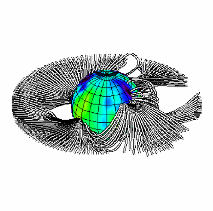
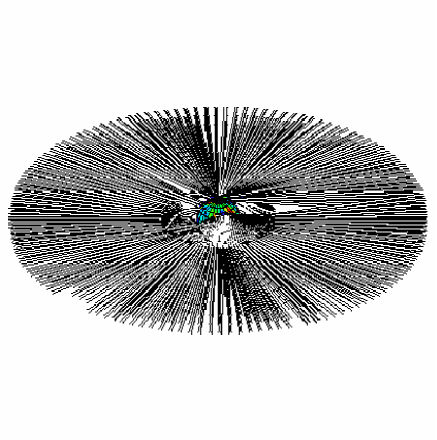
Figure 1: Field lines which could support accretion flows for a model of a CTTS with a field topology that resembles (a) LQ Hya, obtained using the DF Tau parameters from Table 1, and (b) AB Dor using the CY Tau parameters. The stellar surface is coloured to show the strength of the radial component of the field, with red representing 1kG and black -1kG. Field lines have been drawn from the corotation radius. For the lower mass star, DF Tau, the natural extent of its corona would be beyond corotation and therefore there is a mixture of open and closed field lines threading the disc at $R_{co}$. The higher mass star, CY Tau, has a more compact corona and material flows along open field lines from corotation.

2.1 Coronal extent

We determine the maximum possible extent of the corona (which is the extent of the source surface) by determining the maximum radius at which a magnetic field could contain the coronal gas. Since a dipole field falls off with radius most slowly, we use this to set the source surface. For a given surface magnetogram we calculate the dipole field that has the same average field strength. We then need to calculate the hydrostatic pressure along each field line. For an isothermal corona and assuming that the plasma along the field is in hydrostatic equilibrium then,

$$p_{s}=p_{0}\exp{\left(\frac{1}{c_{s}^{2}}\oint_{s}g_{s}ds\right)},$$ (5)

where $c_{s}$ is the isothermal sound speed and $g_{s}$ the component of the effective gravity along the field line such that, $g_{s}=\mathbf{g}\cdot\mathbf{B}/|\mathbf{B}|$, $p_{0}$ is the gas pressure at a field line foot point and $p_{s}$ the pressure at some point along the field line. The effective gravity in spherical coordinates for a star with rotation rate $\omega$ is,

$$\mathbf{g}\left(r,\theta,\phi\right)=\left(-\frac{GM_{\ast}}{r^{2}}+\omega^{2}r\sin^{2}{\theta},\omega^{2}r\sin{\theta}\cos{\theta},0\right).$$ (6)

We can then calculate how the plasma $\beta$, the ratio of gas to magnetic pressure, changes along each field line. If at any point along a field line $\beta>1$ then we assume that the field line is blown open. This effect is incorporated into our model by setting the coronal (gas) pressure to zero whenever it exceeds the magnetic pressure ($\beta>1$). We also set the coronal pressure to zero for open field lines, which have one foot point on the star and one at infinity. The gas pressure, and therefore the plasma $\beta$, is dependent upon the choice of $p_{0}$ which is a free parameter of our model. Jardine et al. (2006) provide a detailed explanation of how $p_{0}$, the coronal base (gas) pressure, can be scaled to the magnetic pressure at a field line foot point, so we provide only an outline here. We assume that the base pressure is proportional to the magnetic pressure then $p_{0}=KB_{0}^{2}$, a technique which has been used successfully to calculate mean coronal densities and X-ray emission measures for the Sun and other main sequence stars (Jardine et al. 2002a, b). By varying the constant $K$ we can raise or lower the overall gas pressure along field line loops. If the value of $K$ is large many field lines would be blown open and the corona would be compact, whilst if the value of $K$ is small then the magnetic field is able to contain more of the coronal gas. The extent of the corona therefore depends both on the value of $K$ and also on $B_{0}$ which is determined directly from surface magnetograms. For an observed surface magnetogram the base magnetic pressure $B_{0}$ varies across the stellar surface, and as such so does the base pressure $p_{0}$ at field line foot points. By considering stars from the COUP dataset Jardine et al. (2006) obtain the value of $K$ which results in the best fit to observed X-ray emission measures, for a given surface magnetogram (see their Table 1). We have adopted the same values in this paper. We then make a conservative estimate of the size of a star’s corona by calculating the largest radial distance at which a dipole field line would remain closed, which we refer to as the source surface $R_{s}$.

2.2 Coronal stripping

Lower mass stars, which have small surface gravities and therefore large pressure scale heights, typically have more extended coronae which would naturally extend beyond the corotation radius. Closed field lines threading the disc beyond corotation would quickly be wrapped up and sheared open. Therefore if the maximum extent of a star’s corona is greater than the corotation radius then we set it to be the corotation radius instead. Higher mass stars, with their larger surface gravities, typically have more compact coronae which may not extend as far as the corotation radius. Therefore if we assume that the disc is truncated at corotation, then accretion proceeds from the inner edge of the disc along radial open field lines. Jardine et al. (2006) provide a discussion about the extent of T Tauri coronae relative to corotation radii. It is also worth noting that Safier (1998) criticises current magnetospheric accretion models for not including the effects of a stellar corona. He argues that the inclusion of a realistic corona blows open most of the closed field with the eventual net effect being that the disc would extend closer to the star. However, in our model there are open field lines threading the disc at corotation and it is therefore reasonable to assume that they are able to carry accretion flows.

Table 1: Data for CTTSs from Valenti & Johns-Krull (2004)

$Star$	$M_{\ast}(M_{\odot})$	$R_{\ast}(R_{\odot})$	$P_{rot}(d)$	$R_{co}(R_{\ast})$
DF Tau	0.17	3.9	8.5	2.47
CY Tau	0.58	1.4	7.5	9.55

2.3 Field extrapolations

The initial field extrapolation yields regions of open and closed field lines. Of these, some intersect the disc and may be actively accreting. For closed field lines which do not intersect the disc it is possible to calculate the X-ray emission measure in the same way as Jardine et al. (2006). To determine if a field line can accrete we find where it threads the disc and calculate if the effective gravity along the path of the field line points inwards, towards the star. From this subset of field lines we select those which have $\beta<1$ along their length. In other words, for any given solid angle we assume that accretion can occur along the first field line within the corotation radius which is able to contain the coronal plasma. We assume that the loading of disc material onto the field lines is infinitely efficient, such that the first field line at any azimuth which satisfies the accretion conditions will accrete, and that field lines interior to this are shielded from the accretion flow. We also assume that the accreting field is static and is therefore not distorted by the disc or by the process of accretion. In §3.3 we consider in more detail how to determine which field lines are able to support accretion flows, in order to calculate mass accretion rates and accretion filling factors.

Fig. 1 shows the first set of field lines which may be accreting, obtained by surrounding the field extrapolations of LQ Hya and AB Dor with a thin wedge-shaped accretion disc, with an opening angle of approximately 10°. In §3 we develop a model for isothermal accretion flows where material leaves the disc at a low subsonic speed, but arrives at the star with a large supersonic speed. Not all of the field lines in Fig. 1 are capable of supporting such accretion flows, and instead represent the maximum possible set of field lines which may be accreting. We assume a coronal temperature of 10MK and obtain the gas pressure at the base of each field line as discussed in §2.1 and by Jardine et al. (2006). The natural extent of the corona of DF Tau would be beyond the corotation radius and therefore accretion occurs along a mixture of closed and open field lines from corotation. One suggestion for how accretion may proceed along open field lines is that an open field line which stretches out into the disc, may reconnect with another open field line for long enough for accretion to occur, only to be sheared open once again. This is of particular importance for the higher mass stars, such as CY Tau, where in some cases we find that the inner edge of the disc is sitting in a reservoir of radial open field lines. This may have important implications for the transfer of torques between the disc and star. However more work is needed here in order to develop models for accretion along open field lines.

These field extrapolations suggest that accretion may occur along field lines that have very different geometries. Indeed, a substantial fraction of the total mass accretion rate may be carried on open field lines. Before developing a detailed model of the mass accretion process, however, we first consider the simple case of a tilted dipole. While this is an idealisation of the true stellar field it allows us to clarify the role that the geometry of the field may have in governing the mass accretion process.

3 Accretion to a dipole

We have constructed two simple analytic models as sketched in Fig. 2. The first case is for a star with a dipolar field with the dipole moment $\mn@boldsymbol{\mu}$ aligned with the stellar rotation axis $\mathbf{\Omega}$. In standard spherical coordinates this field may be described as,

$$\mathbf{B}=\left(\frac{2\mu}{r^{3}}\cos{\theta},\frac{\mu}{r^{3}}\sin{\theta},0\right),$$ (7)

a scenario that allows us to model accretion flows along field lines in the star’s meridional plane. If we then take this field structure and tilt it by $\pi/2$ radians such that $\mn@boldsymbol{\mu}$ now lies in the star’s equatorial plane, perpendicular to $\mathbf{\Omega}$, then those field lines which ran north-south in the meridional plane, now lie east-west in the equatorial plane, with,

$$\mathbf{B}=\left(\frac{2\mu}{r^{3}}\cos{\phi},0,\frac{\mu}{r^{3}}\sin{\phi}\right).$$ (8)

Throughout we shall refer to these cases as the perpendicular dipole for the tilted dipole field and the aligned dipole for the aligned dipole field. To do this we consider steady isothermal accretion flows from a thin accretion disc oriented such that the disc normal is parallel to the stellar rotation axis. An initial sonic Mach number, ${\cal M}$, is ascribed to the accreting material. We then calculate the pressure and velocity profiles, relative to arbitrary initial conditions defined at the disc plane. We calculate the ratio of pressure $p$ at each point along a field line, relative to that at the disc, $p_{d}$; and then from this we calculate how the Mach number of the flow changes along the field.

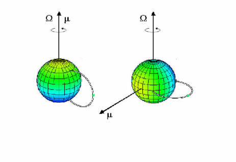
Figure 2: An aligned and tilted dipole field geometry. The aligned dipole (left) with a field line in the star’s meridional plane, with the dipole moment $\mn@boldsymbol{\mu}$ aligned with the stellar rotation axis $\mathbf{\Omega}$, and the perpendicular dipole (right) with a field line in the star’s equatorial plane, with $\mn@boldsymbol{\mu}$ perpendicular to $\mathbf{\Omega}$. The average surface field strength matches that considered by Jardine et al. (2006) with yellow (blue) representing the positive (negative) magnetic pole.

The path of a field line may be described by

$$\frac{B_{r}}{dr}=\frac{B_{\theta}}{rd\theta}=\frac{B_{\phi}}{r\sin{\theta}d\phi}.$$ (9)

For the perpendicular dipole, where $\theta=\pi/2$ for all field lines that pass through the disc, it is quickly established that,

$$\sin^{2}{\phi}=\Psi r,$$ (10)

where $\Psi$ is a constant along a particular field line, such that different values of $\Psi$ correspond to different field lines. For the perpendicular dipole case, at $r=R_{d}$, the maximum radial extent of the field line, $\phi=\pi/2$; thus, $\Psi=1/R_{d}$. Using this result the magnitude of the magnetic field at a point along a field line a distance $r$ from the centre of the star, relative to that at the disc, may be obtained from (8),

$$\frac{B}{B_{d}}=\left(\frac{R_{d}}{r}\right)^{3}\sqrt{\left(4-\frac{3r}{R_{d}}\right)},$$ (11)

where $B_{d}=B\left(r=R_{d}\right)$. An identical expression can be derived for the aligned dipole case.

3.1 Steady isothermal accretion flows

The momentum equation for a steady inviscid flow along a flux tube is

$$\rho\left(\mathbf{v}\cdot\nabla\right)\mathbf{v}=-\nabla\left(p+\frac{B^{2}}{2\mu}\right)+\frac{1}{\mu}\left(\mathbf{B}\cdot\nabla\right)\mathbf{B}+\rho\mathbf{g}_{eff}-2\rho\mathbf{\mn@boldsymbol{\omega}}\times\mathbf{v},$$ (12)

where the symbols have their usual meaning with $\mathbf{g}_{eff}$ being the sum of the gravitational and centrifugal accelerations. In a frame of reference rotating with the the star the effective gravity is,

$$\mathbf{g}_{eff}=\mathbf{g}-\mathbf{\mn@boldsymbol{\omega}}\times\left(\mathbf{\mn@boldsymbol{\omega}}\times\mathbf{r}\right).$$ (13)

The component of the momentum equation along a field line is then,

$$\rho\frac{d}{ds}\left(\frac{v^{2}}{2}\right)=-\frac{dp}{ds}+\rho\mathbf{g}_{eff}\cdot\mathbf{\hat{s}},$$ (14)

since the Coriolis term ($-2\rho\mn@boldsymbol{\omega}\times\mathbf{v}$) does not contribute for flows along the field, and where $\mathbf{\hat{s}}(\mathbf{r})$ is a unit vector along the path of the field line. Throughout terms with a subscript $d$ will denote quantities defined at the disc; for example $\rho_{d},p_{d},v_{d}$ and $B_{d}$ are respectively the density, pressure, velocity along the field and the magnetic field strength as defined at the plane of the disc, a radial distance $R_{d}$ from the centre of the star. Integrating equation (14) from the disc plane to some position along the field line at a distance $r$ from the stellar centre, and using the isothermal equation of state for an ideal gas, $p=\rho c_{s}^{2}$, gives,

$$\ln{\left(\frac{p}{p_{d}}\right)}=\frac{1}{c_{s}^{2}}\left[-\frac{1}{2}\left(v^{2}-v_{d}^{2}\right)+\int\mathbf{g}_{eff}\cdot\mathbf{\hat{s}}ds\right],$$ (15)

where $c_{s}$ is the isothermal sound speed. If we assume that both mass and magnetic flux are conserved along each flux tube (of cross-sectional area $A$), then the flow must satisfy

$$\frac{d}{ds}\left(\rho vA\right) = 0$$ (16)

$$\frac{d}{ds}\left(BA\right) = 0,$$ (17)

which may be expressed equivalently as,

$$\frac{pv}{B}=\frac{p_{d}v_{d}}{B_{d}}=const,$$ (18)

By combining (15) with (18) a relation for the pressure structure along an accreting field line can be established,

$$\ln{\left(\frac{p}{p_{d}}\right)}+\frac{1}{2}{\cal M}^{2}\left(\frac{p_{d}}{p}\frac{B}{B_{d}}\right)^{2}-\frac{1}{2}{\cal M}^{2}-\frac{1}{c_{s}^{2}}\int\mathbf{g}_{eff}\cdot\mathbf{\hat{s}}ds=0,$$ (19)

and also directly from (18) an expression for the velocity structure,

$$\frac{v}{c_{s}}={\cal M}\frac{p_{d}}{p}\frac{B}{B_{d}},$$ (20)

where in both cases ${\cal M}=v_{d}/c_{s}$ denotes the initial sonic Mach number at which the accretion flow leaves the plane of the disc. It is then possible to find the pressure at each point along a field line, relative to the pressure at the disc ($p/p_{d}$), by finding the roots of (19). Once these roots have been found the velocity profile can be obtained from (20) by calculating how the Mach number of the flow varies as material moves from the disc to the star.

3.2 Pressure and velocity profiles

Figure 3: The resulting pressure and velocity profiles for accretion along equatorial dipole field lines. The inner edge of the disc is at $R_{d}=6.0R_{\ast}$ which is approximately the corotation radius. Different lines represent different initial velocities.

For the perpendicular dipole, in the star’s equatorial plane, the effective gravity has only a radial component,

$$\mathbf{g}_{eff}=\left(-\frac{GM_{\ast}}{r^{2}}+\omega^{2}r\right)\mathbf{\hat{r}}.$$ (21)

Taking the component of the effective gravity along the field, that is along a path parameterised by $\mathbf{\hat{s}}=\mathbf{B}/B$, substituting into (19), and using (11) gives an expression for the pressure structure along equatorial field lines,

$$\ln{\left(\frac{p}{p_{d}}\right)}+\frac{1}{2}{\cal M}^{2}\left(\frac{R_{d}}{r}\right)^{6}\left(4-\frac{3r}{R_{d}}\right)\left(\frac{p_{d}}{p}\right)^{2}-\frac{1}{2}{\cal M}^{2}$$

$$+\Phi_{g}\left(\frac{1}{R_{d}}-\frac{1}{r}\right)+\Phi_{c}\left(R_{d}^{2}-r^{2}\right)=0,$$ (22)

where both $r$ and $R_{d}$ are measured in units of the stellar radius $R_{\ast}$ and $\Phi_{g}$ and $\Phi_{c}$ are the surface ratios of the gravitational and centrifugal energies to the thermal energies,

$$\Phi_{g} = \frac{GM_{\ast}}{R_{\ast}c_{s}^{2}}$$ (23)

$$\Phi_{c} = \frac{1}{2}\left(\frac{\omega R_{\ast}}{c_{s}}\right)^{2}.$$ (24)

The roots of (22) give the pressure at some point along a field line loop which is a radial distance $r$ from the stellar centre.

For the aligned dipole, in the star’s meridional plane, the effective gravity has both an $r$ and $\theta$ component,

$$\mathbf{g}_{eff}=\left(-\frac{GM_{\ast}}{r^{2}}+\omega^{2}r\sin^{2}{\theta}\right)\mathbf{\hat{r}}+\left(\omega^{2}r\sin{\theta}\cos{\theta}\right)\hat{\mn@boldsymbol{\theta}}.$$ (25)

Following an identical argument to that above it can be established that for accretion in the star’s meridional plane, the pressure function (19) becomes,

$$\ln{\left(\frac{p}{p_{d}}\right)}+\frac{1}{2}{\cal M}^{2}\left(\frac{R_{d}}{r}\right)^{6}\left(4-\frac{3r}{R_{d}}\right)\left(\frac{p_{d}}{p}\right)^{2}-\frac{1}{2}{\cal M}^{2}$$

$$+\Phi_{g}\left(\frac{1}{R_{d}}-\frac{1}{r}\right)+\Phi_{c}\left(R_{d}^{2}-\frac{r^{3}}{R_{d}}\right)=0.$$ (26)

The only difference from the perpendicular dipole is in the final term.

For a CTTS with a mass of 0.5M_⊙, radius 2R_⊙ and a rotation period of 7 days we have calculated the pressure and velocity structure along accreting dipole field lines, for a range of accretion flow temperatures, starting radii and initial sonic Mach numbers. Figs. 3 and 3 show a typical pressure and velocity profile for the perpendicular dipole, whilst those for the aligned dipole are qualitatively similar. The pressure profile shows how the ratio $p/p_{d}$, where $p$ is the pressure along the field line and $p_{d}$ the pressure at the disc, varies as the flow moves from the disc to the star (plotted logarithmically for clarity). The velocity profile shows how the Mach number of the flow changes along the field line. For different accretion flow temperatures and starting radii the resulting profiles are similar, except in a few select cases, as discussed in the next section. Fig. 3 is for an accretion flow leaving the disc at $R_{d}=6.0R_{\ast}$, which is approximately the equatorial corotation radius $R_{co}$ where,

$$R_{co}=\left(\frac{GM_{\ast}}{\omega^{2}}\right)^{1/3},$$ (27)

and for an accretion flow temperature of 10⁵K. This is at least one order of magnitude higher than what is believed to be typical for accretion in CTTSs, but a higher temperature has been selected here in order to clearly illustrate the various types of solutions labelled in Fig. 3. At lower temperatures the form of the velocity solutions is similar.

At the critical radius $r_{c}$ either the flow velocity equals the sound speed, $v=c_{s}$, or $dv/ds=0$. There are several distinct velocity solutions labelled in Fig. 3. For very small subsonic initial Mach numbers (curve A) the flow remains subsonic all the way to the star, and for large supersonic initial Mach numbers, it remains supersonic from the disc to the star (curve B). There is also a range of initial Mach numbers (curves C) where the flow will not reach the star, and one value of ${\cal M}$ that results in a transonic solution – where the flow leaves the disc at a subsonic speed and accelerates hitting the star at a supersonic speed (curve E). Observations of the widths of line profiles suggest that the accreting material reaches the stellar surface at several hundred kms^-1, certainly at supersonic speeds (e.g. Edwards et al. 1994). The velocity profiles indicate that it is possible to have accretion flows which leave the disc at a low subsonic velocity but which arrive at the star with a large supersonic velocity. In Fig. 3 the transonic solution arrives at the star with a Mach number of 6.54, which at a temperature of 10⁵K corresponds to an in-fall velocity of 243kms^-1. For a realistic accretion temperature of 10⁴K the in-fall velocity is 259kms^-1.

Models of funnel flows have been studied using an isothermal equation of state (Li & Wilson, 1999) and for a polytropic flow (Koldoba et al., 2002), with the latter demonstrating that transonic accretion flows are only possible for a range of starting radii around the corotation radius. MHD simulations by Romanova et al. (2002) also indicate that accretion flows can arrive at the star with large supersonic velocities. However, our aim here is to determine whether or not the magnetic field geometry has any affect on accretion; in particular how the field structure affects the mass accretion rate, rather than to discuss the types of velocity solutions that we would expect to observe. In Appendix A we discuss an efficient algorithm which allows us to determine both the location of the sonic point on a field line and the initial Mach number required to give a smooth transonic solution. This algorithm may be applied to accretion flows along field lines of any size, shape and inclination, even in the absence of analytic descriptions of the magnetic field and effective gravity.

3.3 Mass accretion rates and filling factors

Figure 4: (a) The change in mass accretion rate and (b) the accretion filling factor as a function of $\beta$, for accretion to dipole fields where $\beta$ is the obliquity - the angle between the rotation and magnetic poles, for accretion flow temperatures of 1000K (solid), 2500K (dotted), 5000K (short dash), 7500K (long dash) and 10000K (dash-dot). (c) and (d) show how the contribution to the accretion filling factor from accreting closed and open field changes with $\beta$. The DF Tau parameters from Table 1 have been used. There are no open accreting field lines for the $T_{acc}=1000K$ case.

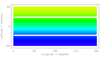
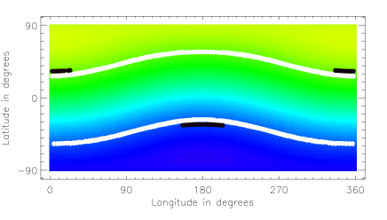
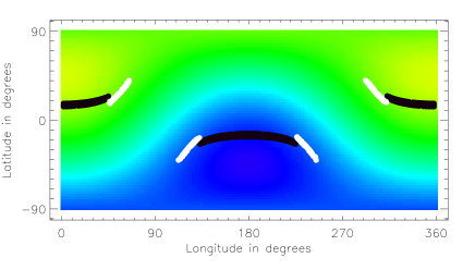
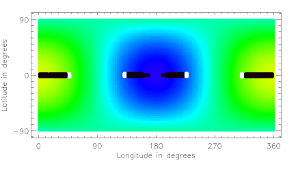
Figure 5: The stellar surface with white (black) points indicating the closed (open) accreting field line foot points for accretion to a dipole with obliquity (a) $\beta=0\degr$, the aligned dipole, where accretion proceeds onto two rings in opposite hemispheres; (b) $\beta=15\degr$ where the accretion rings have been distorted and open field lines produce the small bands centred on 180°and 360°longitude; (c) $\beta=45\degr$ where accretion occurs predominantly along the open field lines and (d) $\beta=90\degr$, the perpendicular dipole, where accretion occurs in bars around the star’s equator. All are for an accretion flow temperature of 10⁴K. The average surface field strength matches that considered by Jardine et al. (2006) with yellow (blue) representing the positive (negative) magnetic pole.

For accretion to occur the effective gravity at the point where a field line threads the disc must point inwards towards the star. From this subset of field lines we select those which are able to contain the corona and support transonic accretion flows. We further check to ensure that the plasma beta resulting from accretion remains $<1$ along their length. Therefore, at any particular azimuth, accretion occurs along the first field line at, or slightly within, the corotation radius; the field line must be able to contain the coronal plasma and have a sonic point along its length. In order to determine if a field line can support a transonic accretion flow, the first step is to find the pressure and velocity structure its length, which will be similar to those described in §3.2. To do this we need to determine the initial Mach number that would produce an accretion flow. We can achieve this by determining if a field line has a sonic point as discussed in Appendix A.

To calculate a mass accretion rate we require the velocity and density of each accretion flow at the stellar surface, and also the surface area of the star covered in hot spots. For an assumed accretion flow temperature we determine the initial Mach number required to generate a transonic velocity profile, along each field line, and determine the in-fall velocity from (20). At every point along a field line we know the ratio of pressure at that point, to that at the disc, $p/p_{d}$. For an isothermal equation of state $p\propto\rho$, so we also know the ratio of densities $\rho/\rho_{d}$ at every point along the accreting field line. Thus for a given disc midplane density $\rho_{d}$, we can estimate the density at the stellar surface $\rho_{\ast}$. Throughout we assume a constant disc midplane density of $\rho_{d}=5.0\times 10^{-9}gcm^{-3}$, a resonable value at the corotation radius for T Tauri stars (e.g. Boss 1996). The mass accretion rate may be expressed in terms of quantities defined at the disc plane, with $\dot{M}\propto\rho_{d}$. Therefore raising or lowering $\rho_{d}$ directly increases or decreases $\dot{M}$. We estimate the total surface area of the star covered in accretion hot spots by summing the area of individual grid cells which contain accreting field line foot points. For each grid cell $i$ (of area $A_{i}$) on the stellar surface we obtain the average in-fall velocity $\bar{v}_{\ast}$ and average density $\bar{\rho}_{\ast}$ of material accreting into that cell. Most grid cells do not contain any accreting field line foot points and therefore do not contribute to the mass accretion rate. The mass accretion rate is then the sum over all cells $i$ containing accreting field line foot points,

$$\dot{M}=\sum_{i}\dot{M}_{i}=\sum_{i}\left[A\bar{v}_{\ast}\bar{\rho}_{\ast}\right]_{i}.$$ (28)

The mass accretion rate can be expressed equivalently as $\dot{M}=\rho_{d}v_{d}A_{d}$, where $A_{d}$ is the surface area of the disc that contributes to accretion (which depends on the radial extent of accreting field lines within the disc). Using the surface area of grid cells within the disc which contain accreting field lines to estimate $A_{d}$, we obtain $\dot{M}$ values that are comparable to those calculated from (28). Therefore it makes little difference which formulation for $\dot{M}$ is used. The accretion filling factor $f_{acc}$, the fractional surface area of the star covered in hot spots, is then calculated from,

$$f_{acc}=\frac{\sum_{i}A_{i}}{4\pi R_{\ast}^{2}}$$ (29)

We have calculated the total mass accretion rate that dipole fields can support for isothermal accretion flow temperatures of between 10³K and 10⁴K; for values of $\beta$ from 0°to 90°, where $\beta$ is the obliquity of the dipole (the angle between the dipole moment and the stellar rotation axis); for the DF Tau parameters in Table 1 and for a coronal temperature of 10MK (see Fig. 4). $\beta=0\degr$ and $\beta=90\degr$ correspond to the aligned and perpendicular dipoles respectively.

For dipolar accretion we obtain typical mass accretion rates of $\dot{M}\approx 10^{-9}-10^{-8}M_{\odot}yr^{-1}$. The mass accretion rate increases with temperature in all cases, but at low accretion temperatures $T_{acc}$, there is little difference in $\dot{M}$ for all values of $\beta$ (see Fig. 4). For higher $T_{acc}$ values, the aligned dipole field can support mass accretion rates which are a factor of two times less than those fields with large values of $\beta$. This, in part, can be attributed to the increase in the amount of open field lines which thread the disc, and are able to support accretion as $\beta$ is increased (see Fig. 4). As the dipole is tilted from $\beta=0\degr$ to $10\degr$ the mass accretion rate is reduced (see Fig. 4). This can be understood by the changing shape of the closed field lines as $\beta$ is increased. For accretion along aligned dipole field lines, accreting material may flow along two identical paths from the disc to the star; that is it may accrete either onto the northern, or the southern hemisphere. Once the dipole has been tilted through a small angle, the path along the field onto each hemisphere changes, with one segment of the closed field line loop being shallower than before and curved towards the star, and the other being longer. This longer segment bulges out slightly, so that material flowing along such field lines follows a path which initially curves away from the star, before looping back around to the stellar surface. This creates a difference in initial Mach numbers necessary to create transonic accretion flows along the different field line segments, with the net result that some closed field line segments are no longer able to accrete transonically when $\beta=10\degr$ (see Fig. 4). As the dipole is tilted further from $\beta=10\degr$ to $\approx 30\degr-40\degr$ the mass accretion rate increases in all but the lowest $T_{acc}$ cases. This is because once the dipole has been tilted far enough the open field lines (those that have foot points at latitudes closer to the magnetic axis) begin to intersect the disc (see Fig. 4). There are therefore more possible paths that material can take from the disc to the star, causing an increase in $\dot{M}$ (again in all but the lower $T_{acc}$ cases). As $\beta$ is further increased the amount of accreting closed field lines continues to reduce, whilst the amount of open field lines threading the disc reaches a maximum, and we therefore see a trend of falling mass accretion rates towards the largest values of $\beta$.

The accretion flow temperature is important in determining whether open field lines are able to support transonic accretion flows. From Figs. 4 and 4 it is clear that the contribution to accretion from the closed field is constant for all values of $T_{acc}$, whereas the contribution from the open field depends strongly on $T_{acc}$, with more open field lines accreting at higher accretion flow temperatures. At the lowest accretion flow temperature which we consider (1000K), there are no open field lines able to support transonic accretion, even for the large values of $\beta$ where there are many such field lines passing through the disc. This can be understood as follows. For transonic accretion a sonic point must exist on a field line. At a sonic point $v=c_{s}$; applying this to (20), substituting into (19) and rearranging gives,

$$\frac{1}{v}\frac{dv}{ds}\left(v^{2}-c_{s}^{2}\right)=\mathbf{g}_{eff}\cdot\mathbf{\hat{s}}-\frac{c_{s}^{2}}{B}\frac{dB}{ds},$$ (30)

from which it can be seen that there exists some critical radius $r_{c}$ where either $v=c_{s}$ or $dv/ds=0$. Clearly at this critical radius the two terms on the RHS of (30) must be equal,

$$\frac{c_{s}^{2}}{B}\frac{dB}{ds}=\mathbf{g}_{eff}\cdot\mathbf{\hat{s}},$$ (31)

where all the terms are evaluated at $r_{c}$. It should be noted that (31) may also be obtained by finding the maximum turning point of (37), consistent with our argument in Appendix A.

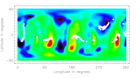
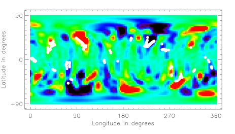
Figure 6: Surface magnetograms as used in Fig. 1 for (a) the LQ Hya-like and (b) the AB Dor-like magnetic fields, coloured to show the strength of the radial component of the field with red representing 1kG and black -1kG. White points are the accreting field line foot points and give an indication of the location of hot spots. Hot spots span a range of latitudes and longitudes; this is in contrast for accretion to a dipole field where the accreting field line foot points would be at high latitudes towards the poles. The accretion filling factor is about 2% in both examples.

The condition for a sonic point to exist on any field line, open or closed, may be expressed as equation (31). $\mathbf{\hat{s}}$ is a unit vector along the path of the field which may be written as $\mathbf{\hat{s}}=\mathbf{B}/B$, which we can use to rewrite (31) as,

$$c_{s}^{2}\frac{dB}{ds}=\mathbf{g}_{eff}\cdot\mathbf{B}.$$ (32)

From this it can be seen that the condition for a sonic point to exist depends on three things: first, the path that a field line takes through the star’s gravitational potential well; second, how quickly the strength of the magnetic field varies as the flow moves along the field line and third, the accretion flow temperature which enters through the sound speed, where for isothermal accretion $c_{s}^{2}\propto T$. It is the interplay between all three of these factors which determines if a sonic point exists.

For low accretion temperatures the sound speed $c_{s}$ is small, whilst for open field lines the $\mathbf{g}_{eff}\cdot\mathbf{B}$ on the RHS of (32) is usually larger than for closed field lines. This can be seen by considering the simple example of a closed dipolar field line and a radial open field line threading the disc at the same point $R_{d}$. For both field lines the effective gravity vector $\mathbf{g}_{eff}$ at $R_{d}$ is the same. For the radial open field line the magnetic field vector $\mathbf{B}$ is aligned with $\mathbf{g}_{eff}$, whereas for the closed dipolar field line, which threads the disc at a large angle, there is some angle $\theta$ between it and $\mathbf{B}$. Hence the scalar product $\mathbf{g}_{eff}\cdot\mathbf{B}=gB\cos{\theta}$ is larger for the open field line. Thus for open field lines the RHS of (32) is larger compared to closed field lines, and therefore a higher accretion flow temperature is required to create the necessary high value of $c_{s}$ in order to balance the two sides of equation (32). Of course, for reasons discussed above, $dB/ds$ is larger for the radial field line, but it is not large enough to compensate for the $\mathbf{g}_{eff}\cdot\mathbf{B}$ term being so small. At higher values of the accretion flow temperature more open field lines are able to accrete, thus helping to increase the mass accretion rate even though the number of closed accreting field lines is significantly less compared to an aligned dipole field.

The aligned dipole field has an accretion filling factor of just under 4% (see Fig. 4), with the $\beta=15\degr$ case having the largest filling factor due to the shape of the closed field lines threading the disc, which allows material to be channelled onto a larger area of the stellar surface. More accreting open field lines means a larger fraction of the star is covered in accreting field line foot points thus increasing the $f_{acc}$ at large accretion flow temperatures. However, when $\beta$ becomes larger as we tilt the dipole further onto its side, $f_{acc}$ decreases. As the field is tilted fewer closed field lines are available for accretion as they no longer intersect the disc (see Fig. 4), leading to a decrease in the filling factor (see Fig. 4). The accretion filling factor is smallest for the perpendicular dipole where material is accreted onto bars about the star’s equator (see Fig. 5), compared to the accretion rings about the poles obtained with the aligned dipole.

We therefore conclude that by considering accretion to tilted dipolar magnetic fields both the mass accretion accretion rate and the accretion filling factor are dependent on the balance between the number of closed and open field lines threading the disc. If there are many open field lines threading the disc, then a higher accretion flow temperature is required in order for the open field to contribute to $\dot{M}$. At high accretion flow temperatures there is at most a factor of two difference between the mass accretion rate that the aligned dipole can support compared to the tilted dipoles with large values of $\beta$. It appears as though the structure of the magnetic field has only a small role to play in determining the mass accretion rate, at least for purely dipolar fields, however, as is discussed in the next section, the magnetic field geometry is of crucial importance in controlling the location and distribution of hot spots.

4 Accretion to complex magnetic fields

Figure 7: Histograms showing the distribution of in-fall velocities assuming steady state accretion flows at 10⁴K, using the field extrapolations in Fig. 1, corresponding to (a) the LQ Hya-like field and (b) the AB Dor-like field using the DF Tau (solid) and CY Tau (dots) stellar parameters listed in Table 1.

4.1 Distribution of hot spots

Brightness modulations have long been interpreted as evidence for hot spots on CTTSs (e.g. Bouvier et al. 1995). Hot spots are a prediction of magnetospheric accretion models and arise from channelled in-falling material impacting the star at large velocity. The distribution of accretion hot spots and their subsequent effects on photometric variability have been studied by several authors, however, only with dipolar magnetic fields (Wood et al. 1996; Mahdavi & Kenyon 1998; Stassun & Wood 1999; Romanova et al. 2004). We find that complex magnetic field geometries have a large effect on the location of hot spots. The accreting field line foot points are shown in Fig. 6, which represent those field lines in Fig. 1 which satisfy the accretion conditions discussed in §3.3. These give an indication of how different field geometries control the shape, location and distribution of hot spots. We find a series of discrete hot spots which span a range of latitudes and longitudes with typical accretion filling factors of around 2%. This is quite different to what we would expect for accretion to an aligned dipole field, where the accreting field line foot points would be at high latitudes, towards the poles. With the complex magnetic fields presented here hot spots can be at high latitudes, but also often at low latitudes close to the star’s equator. The existence of low latitude hot spots has also been predicted by von Rekowski & Brandenburg (2006) who consider accretion along dynamo generated stellar field lines rather than along dipolar field lines. It is worth noting that the line-of-sight field components inferred from polarisation measurements made using the HeI 5876Å emission line by Valenti & Johns-Krull (2004), are well matched by a simple model of a single hot spot at different latitudes dependent on the particular star. Such observations already suggest that low latitude hot spots may be a common feature of CTTSs.

4.2 In-fall velocities

In Appendix A we discuss an analytic method for calculating the location of the critical radius. This allows us to determine which of the field lines from Fig. 1 have sonic points, and then find a transonic velocity solution, where material leaves the disc at a low subsonic speed but arrives at the stellar surface with a large supersonic speed. The accreting field geometry obtained when considering complex magnetic fields is such that there are many field lines of different size and shape which are able to support accretion flows. This results in a distribution of in-fall speeds, rather than a discrete in-fall speed that would be expected for accretion along aligned dipole field lines. Fig. 7 shows the distributions of in-fall velocities for our two accreting field geometries, and for each set of stellar parameters listed in Table 1, for an accretion flow temperature of 10⁴K and a coronal temperature of 10MK. In both cases the in-fall speeds are large enough to produce hot spots on the stellar surface. We obtain larger in-fall velocities when using the CY Tau parameters, which is a higher mass star, compared to the DF Tau parameters. Material accreting onto larger mass stars will experience a steeper gravitational potential than for accretion onto lower mass stars, and this combined with the larger corotation radii for the larger mass stars, naturally leads to greater in-fall speeds.

The accretion flow temperature has a negligible effect on the average in-fall velocity, for any magnetic field structure. We find that the average in-fall speed remains almost constant as the accretion flow temperature is varied, changing by only a few kms^-1. As the temperature is increased the sonic point of the accretion flow is further from the disc, which reduces the final Mach number by which material is arriving at the star. However this reduction in the final Mach number is caused almost exclusively by the increase in the sound speed at higher temperature, whilst the average in-fall velocity remains constant.

Figure 8: (a). The correlation between mass accretion rate and stellar mass. Previously published values [points] are taken from Rebull et al. (2000); Rebull et al. (2002), Mohanty et al. (2005), Natta et al. (2006) and Muzerolle et al. (2005) which is a collection of data from Gullbring et al. (1998), White & Ghez (2001), White & Basri (2003), Muzerolle et al. (2003), Calvet et al. (2004) and Natta et al. (2004). Using data from the COUP sample of accreting stars (Getman et al., 2005) our accretion model yields mass accretion rates [large circles] that are consistent within the observed scatter. Open circles are values calculated from COUP stars with estimates of $R_{\ast}$, $M_{\ast}$, $P_{rot}$, coronal temperature and a CaII equivalent width measurement, whilst the filled circles are values calculated for stars which are regarded as strongly accreting with W(CaII)$<-1$Å. All quantities have been calculated using the LQ Hya surface map and the higher coronal temperatures derived from the COUP data. (b) shows only those stars which are regarded as strongly accreting with the dashed lines indicating the range in mass covered by such COUP stars.

There is a broader distribution of in-fall velocities when considering the CY Tau stellar parameters compared to the narrow distribution for DF Tau, which is more strongly peaked about a single in-fall velocity (see Fig. 7). We calculate the natural radial extent of DF Tau’s corona $R_{s}$ to be larger than the corotation radius ($R_{s}=2.5R_{\ast}$ for the AB Dor-like field and $2.7R_{\ast}$ for the LQ Hya-like field compared to $R_{co}=2.47R_{\ast}$) and therefore accretion proceeds along a mixture of open and closed field lines which thread the disc at corotation. It can be seen from Fig. 1 that accretion occurs almost exclusively from the corotation radius with a small range of azimuths where there are neither open nor closed field lines threading the disc at corotation, and therefore the disc extends closer to the star. This effect is much greater for the CY Tau parameters as its corotation radius is beyond the natural extent of the corona ($R_{s}=2.7R_{\ast}$ for the AB Dor-like field and $2.9R_{\ast}$ for the LQ Hya-like field compared to $R_{co}=9.55R_{\ast}$). Most of the accretion occurs along radial field lines from corotation. However, at some azimuths there are no open field lines stretching out through the disc at corotation, and therefore the inner disc at those azimuths is much closer to the star, with accretion occurring along the closed field lines loops which constitute the star’s corona. A more complete model would take account of the torques resulting from allowing accretion to occur from well within the corotation radius. We do not account for this in our model, however this only occurs for a very small number of field lines, with the bulk of accretion occuring from corotation. The number of field lines accreting at lower velocity from within corotation is small compared to those accreting from $R_{co}$, with the resulting distribution of in-fall speeds instead reflecting variations in the size and shape of field lines accreting from corotation.

We have found that the structure of these complex magnetic fields and more importantly the stellar parameters (mass, radius, rotation period, coronal temperature) are critical in controlling the distribution of in-fall velocities. Consequently this will affect mass accretion rates, which we discuss below, and also spectral line profiles, which will be the subject of future work.

4.3 Mass accretion rates and stellar mass

To investigate the correlation between mass accretion rate and stellar mass we require a large sample of accreting stars with estimates of stellar mass, radius, rotation period and coronal temperature. The X-ray emission from young stars in the Orion Nebula has been studied by COUP (The Chandra Orion Ultradeep Project), which provides a vast amount of data on accreting stars with estimates of all the parameters required by our model to calculate mass accretion rates. Getman et al. (2005) provides an overview of the observations, and the COUP dataset, which is available from ftp://ftp.astro.psu.edu/pub/gkosta/COUP_PUBLIC/.

Rebull et al. (2000) first noted that the apparent increase in mass accretion rate with stellar mass and that the lack of low mass stars with high $\dot{M}$ was a real effect for stars in the Orion flanking fields. White & Ghez (2001) also noted an apparent $\dot{M}-M_{\ast}$ correlation for stars in Taurus-Auriga, with a large scatter in $\dot{M}$ values, with Rebull et al. (2002) reporting that the correlation also existed for stars in NGC 2264. The correlation was then found to extend across several orders of magnitude in mass with the detection of accretion in low mass T Tauri stars and brown dwarfs (White & Basri, 2003) with Muzerolle et al. (2003) being the first to suggest that $\dot{M}\propto M_{\ast}^{2}$. Subsequent observations by Calvet et al. (2004) indicated that this correlation extended to the higher mass, intermediate mass T Tauri stars with several authors adding data at lower masses from various star forming regions (Natta et al. 2004; Mohanty et al. 2005; Muzerolle et al. 2005), with Natta et al. (2006) adding data from $\rho$-Ophiuchus. There can be as much as three orders of magnitude scatter in the measured mass accretion rate at any particular stellar mass. It should also be noted that mass accretion rate measurements for stars in the Trapezium cluster are not consistent with the $\dot{M}\propto M_{\ast}^{2}$ correlation. Robberto et al. (2004) report $\dot{M}$ values for the Trapezium cluster which are significantly lower than those obtained for stars in Taurus and the Orion flanking fields and suggest that the probable cause is that the discs of lower mass stars are being disrupted by UV radiation from the Trapezium OB stars, causing a large drop in mass accretion rates. Also, Calvet et al. (2004) point out that there is a strong bias against the detection of intermediate mass T Tauri stars ($M_{\ast}=1.5-4M_{\odot}$) with lower mass accretion rates, therefore the exponent of the $\dot{M}-M_{\ast}$ correlation may be less that 2. Further, Clarke & Pringle (2006) demonstrate that currently available data are limited by selection effects at high $\dot{M}$ values (whereby accretion rates cannot be determined when accretion luminosity is greater than stellar luminosity) and also by a lower bound defined by the upper limits of non-detections. Their work therefore suggests that the steep correlation between $\dot{M}$ and $M_{\ast}$ is a natural consequence of detection/selection limitations, and that the true $\dot{M}-M_{\ast}$ correlation may be different.

Using the complex magnetic fields discussed above and assuming an accretion flow temperature of 10⁴K, we have calculated mass accretion rates and accretion filling factors for the COUP sample of stars which have estimates of $M_{\ast}$, $R_{\ast}$, $P_{rot}$, coronal temperature and measurements of the CaII 8542Å line, using the lower coronal temperature, and, for those stars with spectra fitted with a two-temperature model, using the higher coronal temperature as well. We have looked for a correlation between the mass accretion rate and stellar mass of the form $\dot{M}\propto M_{\ast}^{\alpha}$, where $\alpha$ is a constant. In Fig. 8 we have plotted our calculated mass accretion rates from the COUP stars as a function of stellar mass, over-plotted on published values, for the LQ Hya-like magnetic field using the higher coronal temperatures. Preibisch et al. (2005) describe how the equivalent width of the CaII 8542Å line is used as an indicator of accretion for stars in the COUP dataset. They follow the classification discussed by Flaccomio et al. (2003), who assume that stars are strongly accreting if the CaII line is seen in emission with W(CaII)$<-$1Å. Stars with W(CaII)$>$1Å are assumed to be either weak or non-accretors. However, it should be noted that many of the stars in the COUP dataset have W(CaII)$=$0Å, and as such cannot be identified as either accreting or non-accreting. Stassun et al. (2006) discuss, with particular reference to the COUP, how some stars can show clear accretion signatures in H$\alpha$ but without showing evidence for accretion in CaII. Therefore the sample of COUP stars considered in Fig. 8 may not be restricted to actively accreting CTTSs and could also include other non-accreting young stars, such as weak line T Tauri stars, where the disc is rarefied or non-existent, and stars which are surrounded by discs but are not actively accreting at this time. However, we consider all of the available stellar parameters from the COUP dataset in order to demonstrate that our model produces a similar amount of scatter in calculated $\dot{M}$ values. In Fig. 8 we have only plotted those COUP stars which are regarded as strongly accreting based on the equivalent width of the CaII 8542Å line.

By fitting a line to the filled circles in Fig. 8 we find a correlation of the form $\dot{M}\propto M_{\ast}^{1.1}$ for COUP stars which are regarded as strong accretors, using the LQ Hya-like magnetic field. For the AB Dor-like field we find $\dot{M}\propto M_{\ast}^{1.2}$. Therefore our simple steady state isothermal accretion model produces an increase in mass accretion rate with stellar mass, and predicts $\dot{M}$ values which are consistent within the observed scatter, but it underestimates the exponent of 2 obtained from published values. We find similar results when considering both the lower and higher coronal temperatures. However, the strongly accreting COUP stars only include stellar masses of $M_{\ast}\approx 0.1-2.6M_{\odot}$, and as such do not provide a large enough range in mass to test if our accretion model can reproduce the observed correlation. Therefore if we only consider the observational data in the restricted range of mass provided by the COUP dataset (indicated by the vertical dashed lines in Fig. 8) then the exponent of the observed correlation is less than 2, with $\dot{M}\propto M_{\ast}^{1.4}$, and if higher mass stars do exist with lower mass accretion rates, could even be less than 1.4. Therefore our simple model, which Jardine et al. (2006) have successfully used to explain the observed correlation between X-ray emission measure and stellar mass, comes close to reproducing the stellar mass - mass accretion rate correlation. It is also worth noting that our model produces a correlation in agreement Clarke & Pringle (2006).

The accretion filling factors are typically around 2.5% for the sample of COUP stars (see Fig. 9), although it varies from less than 2% to greater than 4%. There is a slight trend for higher mass stars to have smaller filling factors, that is there is a slight trend for stars with larger corotation radii to have a smaller filling factors despite their larger mass accretion rates. For stars with smaller corotation radii (lower mass) there are many field lines threading the disc and able to support accretion, and therefore a large fraction of the stellar surface is covered in accreting field lines foot points, whereas for stars with larger corotation radii (higher mass) there are less accreting field lines and therefore smaller filling factors. However the higher mass stars are accreting at a larger velocity therefore producing larger mass accretion rates. The actual accretion filling factor depends on the magnetic field structure. For the AB Dor-like magnetic field the accretion filling factors are smaller at around 1.8%.

Figure 9: The accretion filling factors are small, and typically around $2.5$% for the LQ Hya-like magnetic field. Open and filled circles represent the same set of stars in Fig. 8.

5 Summary

By considering accretion to both dipolar and complex magnetic fields we have constructed a steady state isothermal accretion model were material leaves the disc at low subsonic speeds, but arrives at the star at large supersonic speeds. We find in-fall velocities of a few hundred kms^-1 are possible which is consistent with measurements of the redshifted absorption components of inverse P-Cygni profiles (e.g. Edwards et al. 1994). We found that for accretion along aligned and perpendicular closed dipole field lines that there was little difference in in-fall speeds between the two cases. However, for tilted dipole fields in general (rather than just considering a single closed field line loop) there are many open and closed field lines threading the disc providing different paths that material could flow along from the disc to the star. The path that a particular field line takes through the star’s gravitational potential combined with the strength of magnetic field and how that changes along the field line path, are all important in determining whether or not a field line can support transonic accretion. At low accretion flow temperatures open field lines are typically not able to support transonic accretion, but at higher accretion flow temperatures they can accrete transonically and consequently we see an increase in the mass accretion rate. We only find a factor of two to three difference in $\dot{M}$ values for accretion to tilted dipolar magnetic fields suggesting that the geometry of the field itself is not as significant as the stellar parameters (which control the position of corotation) in controlling the mass accretion rate.

The magnetic field geometry is crucial in controlling the location and distribution of hot spots on the stellar surface. For accretion to complex magnetic fields we find that hot spots can span a range of latitudes and longitudes, and are often at low latitudes towards the star’s equator. We find that the accretion filling factors (the fractional surface area of a star covered in hot spots) are small and typically around 2.5%, but they can vary from less than 1% to over 4% and rarely to larger values. This is consistent with observations which suggest small accretion filling factors and the inference of hot spots at various latitudes (Valenti & Johns-Krull, 2004).

For accretion with complex magnetic fields there is a distribution of in-fall speeds, which arises from variations in the size and shape of accreting field lines. The resulting effect that this will have on line profiles will be addressed in future work. In our model most of the accretion occurs from the corotation radius, but at some azimuths the disc extends closer to the star meaning that a small fraction of field lines are accreting material at lower velocity. Lower mass stars, with their lower surface gravities, typically have larger coronae which would extend out to corotation (Jardine et al., 2006). Therefore the lower mass stars are accreting along a mixture of open and closed field lines from the corotation radius. In contrast higher mass stars, with their higher surface gravities, have small compact coronae, and so the star is actively accreting along mainly open field lines from the corotation radius. However, such open field lines do not thread the disc at all azimuths, with some accretion instead occuring along field lines which are much closer to the stellar surface. This gives rise to a small peak at low velocity in the in-fall velocity distribution. However, this represents only a small fraction of all accreting field lines which do not contribute significantly to the resulting mass accretion rate.

Finally we applied our accretion model to stars from the COUP dataset which have estimates of the stellar parameters and measurements of the equivalent width of the CaII 8542Å line, which is seen in emission for accreting stars. For the complex magnetic fields we calculated mass accretion rates and accretion filling factors as a function of stellar mass. The observed stellar mass - accretion rate correlation is $\dot{M}\propto M_{\ast}^{2}$ (Muzerolle et al. 2003; Calvet et al. 2004; Mohanty et al. 2005; Muzerolle et al. 2005), however, this may be strongly influenced by detection/selection effects (Clarke & Pringle, 2006). By only considering observational data across the range in mass provided by the COUP sample of accreting stars, the observed correlation becomes $\dot{M}\propto M_{\ast}^{1.4}$. Our steady state isothermal model gives an exponent of 1.1 for the LQ Hya-like magnetic field and 1.2 for the AB Dor-like field with similar results for both the high and low coronal temperatures, with the caveat that the observed correlation may be less than 1.4 due to a strong bias against the detection of higher mass stars with lower mass accretion rates (Calvet et al., 2004). It may be the case that an exponent of 1.2 compared to the observed 1.4, represents the best value that can be achieved with a steady state isothermal accretion model. Jardine et al. (2006) have used this model to reproduce the observed increase in X-ray emission measure with stellar mass (Preibisch et al., 2005). However, they find that when using the complex magnetic fields presented here (extrapolated from surface magnetograms of the young main-sequence stars AB Dor and LQ Hya) they slightly under estimate the emission measure-mass correlation. When they use dipolar magnetic fields, which represent the most extended stellar field, they slightly over estimated the correlation. This suggests that T Tauri stars have magnetic fields which are more extended than those of young main sequence stars, but are more compact than purely dipolar fields.

Also, our model has not been tested across a large enough range in mass to make the comparison with the observed correlation of $\dot{M}\propto M_{\ast}^{2}$. However, it already compares well with the alternative suggestion of Clarke & Pringle (2006) that the $\dot{M}-M_{\ast}$ correlation is not as steep with $\dot{M}\propto M_{\ast}^{1.35}$. In future we will extend our model to consider accretion from the lowest mass brown dwarfs, up to intermediate mass T Tauri stars. This will require estimates of, in particular, rotation periods and coronal temperatures.

Our accretion model reproduces a similar amount of scatter in calculated $\dot{M}$ values compared with observations. This can be attributed to different sets stellar parameters changing the structure of the accreting field. The stellar parameters control the location of the corotation radius, whilst it is the position of corotation relative to the natural coronal extent, which determines whether or not accretion occurs predominantly along the open field. However, for the moment we are restricted to using surface magnetograms of young main sequence stars which may not necessarily represent the true fields of T Tauri stars. It could be possible that variations in magnetic field geometry from star to star are responsible for the observed large scatter in the mass accretion rate at any particular stellar mass. If there is a large difference in the structure of the accreting field from star to star this could lead to large variations in mass accretion rates onto different stars. The spectropolarimeter at the Canada France Hawaii telescope, ESPaDOnS: Echelle SpectroPolarimetric Device for the Observation of Stars (Petit et al. 2003; Donati 2004), will in the near future allow the reconstruction of the magnetic field topology of CTTSs from Zeeman-Doppler imaging. This will allow a number of open questions to be addressed about the nature of the magnetic fields of T Tauri stars and allow us to test if our accretion model can indeed reproduce the stellar mass - accretion rate correlation.

Appendix A Algorithm for finding a sonic point and the initial Mach number required for a smooth transonic solution

In order to determine the initial Mach number which results in a transonic accretion flow we need to understand exactly what the different solutions in Fig. 3 represent. These curves are obtained from the pressure solutions plotted in Fig. 3 using equation (20). These pressure profiles track how the roots of (19) change as the flow moves along a field line. The pressure function (19) can be written in the form,

$$f\left(\frac{p}{p_{d}}\right)=\ln{\left(\frac{p}{p_{d}}\right)}+a\left(\frac{p_{d}}{p}\right)^{2}+b=0,$$ (33)

where $a$ and $b$ are constants at any fixed point along a field line with,

$$a = \frac{1}{2}{\cal M}^{2}\left(\frac{B}{B_{d}}\right)^{2},$$ (34)

$$b = -\frac{1}{2}{\cal M}^{2}-\frac{1}{c_{s}^{2}}\int\mathbf{g}_{eff}\cdot\mathbf{\hat{s}}ds.$$ (35)

For a Mach number prescribed to a flow leaving the disc, the pressure function has two roots, which consequently yield two velocities. One of the roots represents the true physical solution, and the other is a mathematical solution of no physical significance. The branches in Fig. 3 occur in pairs, with an individual branch tracking how one of the pressure roots changes as the flow travels along the field line. For example, suppose we had chosen an initial (subsonic) Mach number which resulted in a purely subsonic flow from the disc to the star (curve A in Fig. 3). Then one of the roots, the one which gives a subsonic solution everywhere along the flow, is the true physical one. The second root of (A1) produces a supersonic solution (curve B), which is of mathematical interest, but has no physical meaning. Conversely, had we chosen the initial Mach number which corresponded to the same supersonic branch, then this purely supersonic branch is the one with physical meaning, with the other root then generating the purely subsonic branch, the mathematical artifact. Thus the purely subsonic and supersonic solutions exist provided our pressure function (33) has two real roots when evaluated at each point along a field line.

At small values of $p/p_{d}$ the second $(p/p_{d})^{-2}$ term in (33) dominates with $f(p/p_{d})\to\infty$ as $p/p_{d}\to 0$. At larger values of $p/p_{d}$ the logarithmic term dominates. Thus (33) has a minimum which occurs when,

$$\frac{p}{p_{d}}={\cal M}\frac{B}{B_{d}}.$$ (36)

For this value of $p/p_{d}$ the pressure function reduces to,

$$f_{c}(r)=\ln{\left({\cal M}\frac{B}{B_{d}}\right)}+\frac{1}{2}-\frac{1}{2}{\cal M}^{2}-\frac{1}{c_{s}^{2}}\int\mathbf{g}_{eff}\cdot\mathbf{\hat{s}}ds,$$ (37)

which we will refer to as the critical function, $f_{c}$. In order for two real roots to exist at some point $r$ along a field line then $f_{c}(r)<0$ must hold. Thus for purely subsonic$/$supersonic solutions to exist then $f_{c}<0$ at each point along a field line, with $f_{c}$ reaching its highest value at the critical radius (where the two roots of the pressure function, and therefore the velocity roots, are closest together). Another pair of solutions are the discontinuous ones labelled C and D in Fig. 3. For these solutions $f_{c}<0$ for $r_{1}<r\leq R_{d}$ and $R_{\ast}\leq r<r_{2}$. However for the domain $r_{2}<r<r_{1}$, $f_{c}>0$, and therefore the pressure function has no real roots, and we cannot satisfy (19); hence there are no velocity solutions for these values of $r$. For $r=r_{1}$ and $r=r_{2}$, $f_{c}=0$, and at these points the pressure function has a single repeated root that coincides with the pressure function minimum.

Figure 10: The location of the critical radius $r_{c}$ as a function of accretion flow temperature $T_{acc}$ for starting radii $R_{d}$ about the corotation radius (upper line, $R_{d}=7.0R_{\ast}$, middle line $R_{d}=6.0R_{\ast}\approx R_{co}$ and lower line $R_{d}=5.0R_{\ast}$). At lower temperatures $r_{c}$ is closer to the inner edge of the disc, and the difference between the aligned and perpendicular dipoles is larger. Variation of the starting radius has little effect for the perpendicular dipole, and is of minor significance for the aligned dipole.

The final pair of solutions are the transonic ones labelled E and F in Fig. 3. Here $f_{c}<0$ for all $r$, except at the sonic point where $r=r_{c}$ and $f_{c}=0$. Hence, for a transonic solution the maximum value of the critical function $f_{c}$ is zero at the critical radius $r_{c}$, but less than zero at all other points along the field line. This then gives us a robust method for finding both the critical radius and the initial Mach number required for a smooth transonic solution (provided such a solution exists).

At the critical radius the minimum of our pressure function is at its highest value; that is $f_{c}$ has a maximum turning point. Hence to determine if a transonic solution exists we select any initial Mach number ${\cal M}$ and calculate how $f_{c}$ varies as we move along a field line from the disc to the star. If a sonic point exists on that field line, $f_{c}$ will have a distinct maximum at some point. The advantage of this method is that it is possible to recover the initial Mach number that would result in a smooth transonic flow, simply by varying ${\cal M}$ until $f_{c}=0$ at $r_{c}$; that is we change ${\cal M}$ until the maximum value of $f_{c}$ occurs at zero. This algorithm is an efficient method for quickly determining both the critical radius and the initial Mach number which results in a transonic accretion flow. Of course, not all field lines have a sonic point (see §3.3) as the critical radius may either be interior to the star or exterior to the starting radius. This algorithm may be applied to accretion flows along field lines of any size, shape and inclination, even in the absence of analytic descriptions of the magnetic field and effective gravity.

The location of the critical radius (or the sonic point for a transonic solution) determines the velocity with which material impacts the stellar photosphere. We have found the critical radius from the maximum value of $f_{c}$ for both the perpendicular and aligned dipoles for a CTTS with a mass of 0.5M_⊙, radius 2R_⊙ and a rotation period of 7 days. For our two dipole cases the $B/B_{d}$ and $\mathbf{g}_{eff}\cdot\mathbf{\hat{s}}$ terms that contribute to (37), have analytic forms given respectively by (11) and either (21) for the perpendicular dipole, or (25) for the aligned dipole; in both cases $\mathbf{\hat{s}}=\mathbf{B}/B$. The location of $r_{c}$ therefore changes as we vary both the starting radius $R_{d}$ and also the temperature (which enters through the sound speed). It should be noted, however, that for certain choices of parameters sometimes $f_{c}$ has no distinct maximum turning point, indicating that either the critical radius is interior to the star ($r_{c}\leq R_{\ast}$), or beyond the starting radius ($r_{c}>R_{d}$). In these cases flows that leave the disc at a subsonic speed remain subsonic all the way to the star, and likewise supersonic flows remain supersonic at all points along a field line.

Fig. 10 shows how the critical radius varies for a range of temperatures and starting radii for both the perpendicular and aligned dipoles. In both cases, the critical radius moves towards the inner edge of the disc with decreasing temperature. In other words as the accretion flow temperature decreases the sonic point moves along the field line away from the star, closer to where the flow leaves the disc. It is straight forward to explain why this should happen by considering a transonic flow which would leave the disc at a subsonic speed. As the temperature drops the sound speed decreases ($c_{s}\propto\sqrt{T}$); therefore a flow leaving the disc does not have to accelerate for as long to reach its own sound speed and becomes supersonic sooner. Thus $r_{c}$ moves closer to $R_{d}$ with decreasing temperature; and for a high enough temperature the critical radius is interior to the star, and conversely for a low enough temperature the critical radius is beyond the starting radius. However, at least for this particular set of stellar parameters, the actual change in critical radius location with temperature is small.

We also found that as the critical radius moved towards the inner edge of the disc, the Mach number with which the flow arrived at the star increased. This would be expected however as the critical radius moves away from the star due to the sound speed decrease, which would naturally increase the flow Mach number at the star (for transonic and purely supersonic flows).

It can be seen from Fig. 10 that for the perpendicular dipole varying the starting radius of the flow, $R_{d}$, has little effect on the location of the critical radius. Therefore changing the size of equatorial field lines has a negligible effect on the velocity with which accretion flows (along the field) reach the star. For the aligned dipole changing where the field lines thread the disc does have an effect on the critical radius location and therefore on the final velocity with which material impacts the star. However, due to the overall small change in the critical radius location evident in Fig. 10 the in-fall velocity only varies by around 6 kms^-1. It therefore appears that the physical size of field lines, in a dipole accretion model, is of little importance for poloidal field lines (aligned north-south in the star’s meridional plane), and is negligible for equatorial field lines (aligned east-west in the star’s equatorial plane).

The effect of the field orientation is also of little importance for closed dipolar field lines. If we have a closed field line in the equatorial plane, with a maximum radial extent $R_{d}$, then changing the inclination of that field line so that it now lies in the meridional plane, has an effect on the critical radius location (see Fig. 10). The only major difference between the two cases enters through the effective gravity, which only has a radial component in the equatorial plane, but both $r$ and $\theta$ components in the meridional plane. However, the difference in in-fall velocities is again very small, at only a few kms^-1. This suggests that for accretion along closed dipolar field lines, where material is leaving the disc at a fixed radius, the field geometry has little effect on in-fall velocities; however, as discussed in §4.2, this result does not hold when we consider more complicated multipolar fields.

References

- Alexander & Armitage (2006) Alexander R. D., Armitage P. J., 2006, ApJL, 639, L83
- Altschuler & Newkirk (1969) Altschuler M. D., Newkirk G., 1969, SoPh, 9, 131
- Basri et al. (1992) Basri G., Marcy G. W., Valenti J. A., 1992, ApJ, 390, 622
- Boss (1996) Boss A. P., 1996, ApJ, 469, 906
- Bouvier et al. (1995) Bouvier J., Covino E., Kovo O., Martin E. L., Matthews J. M., Terranegra L., Beck S. C., 1995, A&A, 299, 89
- Calvet et al. (2004) Calvet N., Muzerolle J., Briceño C., Hernández J., Hartmann L., Saucedo J. L., Gordon K. D., 2004, AJ, 128, 1294
- Clarke & Pringle (2006) Clarke C. J., Pringle J. E., 2006, MNRAS, in press (astro-ph/0604196)
- Collier Cameron & Campbell (1993) Collier Cameron A., Campbell C. G., 1993, A&A, 274, 309
- Daou et al. (2006) Daou A. G., Johns-Krull C. M., Valenti J. A., 2006, AJ, 131, 520
- Donati (1999) Donati J.-F., 1999, MNRAS, 302, 457
- Donati (2004) Donati J. F., 2004, in SF2A-2004: Semaine de l’Astrophysique Francaise ESPaDOnS@CFHT: the new generation stellar spectropolarimeter. pp 217–+
- Donati & Collier Cameron (1997) Donati J.-F., Collier Cameron A., 1997, MNRAS, 291, 1
- Donati et al. (1999) Donati J.-F., Collier Cameron A., Hussain G. A. J., Semel M., 1999, MNRAS, 302, 437
- Donati et al. (2003) Donati J.-F. et al. 2003, MNRAS, 345, 1145
- Donati et al. (1997) Donati J.-F., Semel M., Carter B. D., Rees D. E., Collier Cameron A., 1997, MNRAS, 291, 658
- Edwards et al. (1994) Edwards S., Hartigan P., Ghandour L., Andrulis C., 1994, AJ, 108, 1056
- Flaccomio et al. (2003) Flaccomio E., Damiani F., Micela G., Sciortino S., Harnden F. R., Murray S. S., Wolk S. J., 2003, ApJ, 582, 398
- Getman et al. (2005) Getman K. V. et al. 2005, ApJS, 160, 319
- Guenther et al. (1999) Guenther E. W., Lehmann H., Emerson J. P., Staude J., 1999, A&A, 341, 768
- Gullbring et al. (1998) Gullbring E., Hartmann L., Briceño C., Calvet N., 1998, ApJ, 492, 323
- Hussain et al. (2002) Hussain G. A. J., van Ballegooijen A. A., Jardine M., Collier Cameron A., 2002, ApJ, 575, 1078
- Jardine et al. (2006) Jardine M., Cameron A. C., Donati J.-F., Gregory S. G., Wood K., 2006, MNRAS, 367, 917
- Jardine et al. (2002a) Jardine M., Collier Cameron A., Donati J.-F., 2002a, MNRAS, 333, 339
- Jardine et al. (2002b) Jardine M., Wood K., Collier Cameron A., Donati J.-F., Mackay D. H., 2002b, MNRAS, 336, 1364
- Johns-Krull & Gafford (2002) Johns-Krull C. M., Gafford A. D., 2002, ApJ, 573, 685
- Johns-Krull et al. (1999a) Johns-Krull C. M., Valenti J. A., Hatzes A. P., Kanaan A., 1999a, ApJL, 510, L41
- Johns-Krull et al. (1999b) Johns-Krull C. M., Valenti J. A., Koresko C., 1999b, ApJ, 516, 900
- Koldoba et al. (2002) Koldoba A. V., Lovelace R. V. E., Ustyugova G. V., Romanova M. M., 2002, AJ, 123, 2019
- Königl (1991) Königl A., 1991, ApJL, 370, L39
- Li & Wilson (1999) Li J., Wilson G., 1999, ApJ, 527, 910
- Mahdavi & Kenyon (1998) Mahdavi A., Kenyon S. J., 1998, ApJ, 497, 342
- McIvor et al. (2003) McIvor T., Jardine M., Cameron A. C., Wood K., Donati J.-F., 2003, MNRAS, 345, 601
- McIvor et al. (2004) McIvor T., Jardine M., Cameron A. C., Wood K., Donati J.-F., 2004, MNRAS, 355, 1066
- Mohanty et al. (2005) Mohanty S., Jayawardhana R., Basri G., 2005, ApJ, 626, 498
- Muzerolle et al. (2003) Muzerolle J., Hillenbrand L., Calvet N., Briceño C., Hartmann L., 2003, ApJ, 592, 266
- Muzerolle et al. (2005) Muzerolle J., Luhman K. L., Briceño C., Hartmann L., Calvet N., 2005, ApJ, 625, 906
- Natta et al. (2004) Natta A., Testi L., Muzerolle J., Randich S., Comerón F., Persi P., 2004, A&A, 424, 603
- Natta et al. (2006) Natta A., Testi L., Randich S., 2006, A&A, 452, 245
- O’Sullivan et al. (2005) O’Sullivan M., Truss M., Walker C., Wood K., Matthews O., Whitney B., Bjorkman J. E., 2005, MNRAS, 358, 632
- Padoan et al. (2005) Padoan P., Kritsuk A., Norman M. L., Nordlund Å., 2005, ApJL, 622, L61
- Petit et al. (2003) Petit P., Donati J.-F., The Espadons Project Team 2003, in EAS Publications Series Stellar polarimetry with ESPaDOnS. pp 97–+
- Preibisch et al. (2005) Preibisch T. et al. 2005, ApJS, 160, 401
- Rebull et al. (2002) Rebull L. M. et al. 2002, AJ, 123, 1528
- Rebull et al. (2000) Rebull L. M., Hillenbrand L. A., Strom S. E., Duncan D. K., Patten B. M., Pavlovsky C. M., Makidon R., Adams M. T., 2000, AJ, 119, 3026
- Robberto et al. (2004) Robberto M., Song J., Mora Carrillo G., Beckwith S. V. W., Makidon R. B., Panagia N., 2004, ApJ, 606, 952
- Romanova et al. (2002) Romanova M. M., Ustyugova G. V., Koldoba A. V., Lovelace R. V. E., 2002, ApJ, 578, 420
- Romanova et al. (2004) Romanova M. M., Ustyugova G. V., Koldoba A. V., Lovelace R. V. E., 2004, ApJ, 610, 920
- Safier (1998) Safier P. N., 1998, ApJ, 494, 336
- Shu et al. (1994) Shu F., Najita J., Ostriker E., Wilkin F., Ruden S., Lizano S., 1994, ApJ, 429, 781
- Smith et al. (2003) Smith K., Pestalozzi M., Güdel M., Conway J., Benz A. O., 2003, A&A, 406, 957
- Stassun & Wood (1999) Stassun K., Wood K., 1999, ApJ, 510, 892
- Stassun et al. (2006) Stassun K. G., van den Berg M., Feigelson E., Flaccomio E., 2006, ApJ, in press (astro-ph/0606079)
- Symington et al. (2005) Symington N. H., Harries T. J., Kurosawa R., Naylor T., 2005, MNRAS, 358, 977
- Uchida & Shibata (1984) Uchida Y., Shibata K., 1984, PASJ, 36, 105
- Valenti & Johns-Krull (2004) Valenti J. A., Johns-Krull C. M., 2004, Ap&SS, 292, 619
- van Ballegooijen et al. (1998) van Ballegooijen A. A., Cartledge N. P., Priest E. R., 1998, ApJ, 501, 866
- von Rekowski & Brandenburg (2006) von Rekowski B., Brandenburg A., 2006, Astronomische Nachrichten, 327, 53
- White & Basri (2003) White R. J., Basri G., 2003, ApJ, 582, 1109
- White & Ghez (2001) White R. J., Ghez A. M., 2001, ApJ, 556, 265
- Wood et al. (1996) Wood K., Kenyon S. J., Whitney B. A., Bjorkman J. E., 1996, ApJL, 458, L79+