Constraints on the Accretion History of Massive Black Holes from Faint X-ray Counts

Abstract

We investigate how hierarchical models for the co-evolution of the massive black hole (MBH) and AGN population can reproduce the observed faint X-ray counts. We find that the main variable influencing the theoretical predictions is the Eddington ratio of accreting sources. We compare three different models proposed for the evolution of AGN Eddington ratio, $f_{\rm Edd}$: constant $f_{\rm Edd}=1$, $f_{\rm Edd}$ decreasing with redshift, and $f_{\rm Edd}$ depending on the AGN luminosity, as suggested by simulations of galactic mergers including MBHs and AGN feedback. We follow the full assembly of MBHs and host halos from early times to the present in a $\Lambda$CDM cosmology. AGN activity is triggered by halo major mergers and MBHs accrete mass until they satisfy the observed correlation with velocity dispersion. We find that all three models can reproduce fairly well the total faint X-ray counts. The redshift distribution is however poorly matched in the first two models. The Eddington ratios suggested by merger simulations predicts no turn-off of the faint end of the AGN optical luminosity function at redshifts $z\ga 1$, down to very low luminosity.

1 Introduction

Several hierarchical models for the evolution of the MBH and AGN populations (see,e.g., Haehnelt & Rees, 1993; Haiman & Menou, 2000; Hatziminaoglou et al., 2001; Wyithe & Loeb, 2003; Cattaneo et al., 1999; Kauffmann & Haehnelt, 2000; Cavaliere & Vittorini, 2000; Volonteri et al., 2003; Granato et al., 2004; Lapi et al., 2006) have proved successful in reproducing the AGN optical luminosity function (OLF) in a large redshift range ($1\la z\la 6$). Typically, these models assume that AGN activity is triggered by major mergers. Galactic interactions trigger gas inflows, and the cold gas may be eventually driven into the very inner regions, fueling an accretion episode and the growth of the nuclear MBH. Hydrodynamic simulations of major mergers have shown that a significant fraction of the gas in interacting galaxies falls to the center of the merged system (Mihos & Hernquist, 1994, 1996): the cold gas may be eventually driven into the very inner regions, fueling an accretion episode and the growth of the nuclear BH. This last year has been especially exciting, as the first high resolution simulations of galactic mergers including BHs and AGN feedback, showed that the merger scenario is generally correct (Springel et al., 2005; Di Matteo et al., 2005). In hierarchical models of galaxy formation major mergers are responsible for forming bulges and elliptical galaxies. Support for merger driven activity therefore comes from the observed correlation between bulge luminosity - or stellar velocity dispersion - and black hole mass, suggesting a single mechanism for assembling black holes and forming spheroids in galaxy halos (Magorrian et al., 1998; Marconi et al., 2004; Gebhardt et al., 2000; Ferrarese & Merritt, 2000).

Notwithstanding the success at high redshift, hierarchical models struggle to match the AGN OLF at low redshift ($z\la 1$) by overpredicting the bright end, and underpredicting the faint end of the OLF, as the decrease of the halo merger rate with time is less dramatic than the observed fall of the AGN population. The overprediction of bright AGN can be imputed to inefficient cooling in large halos. Imposing an upper limit to the AGN host halo mass ($\sim 10^{13.5}M_{\odot}$, Wyithe & Loeb (2003); Marulli et al. (2006)) in fact significantly improves the match at the bright end of the OLF.

The under-abundance of faint AGN can be instead attributed to the assumption, common to most models, of very efficient accretion, at rates close to the Eddington rate. Merloni et al. (2003) and Merloni (2004) have shown that low-redshift AGN are probably accreting inefficiently, i.e. both at an accretion rate much smaller than the Eddington rate and with a low radiative efficiency. These considerations suggest that successful predictions for the evolution of AGN luminosity should include more sophisticated models for accretion. A first step in this direction can be taken by considering the results of the recent merger simulations, which track also accretion on a central MBH. Although these simulations lack the necessary resolution for resolving the accretion process in the vicinity of the MBH, empirical models (Hopkins et al., 2005), based on coupling results from the above simulations with the observed LF in the hard X-ray band (HXLF), have been shown to reproduce simulaneously several optical and X-ray observations. The Hopkins et al. (2005) empirical models, however, are not embedded in a cosmological evolutionary framework, that is they derive the MBH population properties at a given time, but not how the population of black holes at an earlier time evolves into the MBHs present at a later time. From the observed HXLF Hopkins et al. (2005) derive the rate at which AGN of a given luminosity at the peak of activity must be created. This information is then used as a proxy for the galaxy merger rate which should provide the boundary conditions for determining the evolution of the MBH population.

We here couple the predictions from Hopkins et al. (2005) with the merger rate expected in the currently favoured cold dark matter scenario. The main novelties of the present investigation with respect to Hopkins et al. (2005), are therefore that (i) the rate of mergers, which trigger AGN activity, is directly derived in the currently favoured cold dark matter (CDM) cosmology. In principle, the empirical merger rate derived by Hopkins et al. (2005) is not granted to correspond to the CDM one. Also, (ii), we grow MBHs in a self-consistent way, that is we trace the whole accretion history of MBHs from early times to the present, requiring continuity in the population.

Our aim is to investigate here to which extent hierarchical models, coupled with the prescriptions based on the above simulations (§1), can reproduce the low-redshift evolution of AGN. We show that reproducing the HXLF is a necessary, but not sufficient, condition for matching the redshift distribution of faint X-ray counts (§2). We identify the redshift distribution of faint X-ray counts as the most sensitive observational result to discriminate between models (§3, §4). Finally, in §5 we summarize the results and discuss their implications.

2 Formation of massive black holes and growth by mass accretion

In our framework pregalactic ‘seed’ holes form at early times. In most of our calculations we follow Volonteri et al. (2003); Volonteri et al. (2005), assuming that seed MBHs form with intermediate masses ($m_{\rm seed}\lid 600\,\,{\rm M_{\odot}}$) in halos collapsing at $z=20$ from rare 3.5-$\sigma$ peaks of the primordial density field (Madau & Rees, 2001) as end-product of the very first generation of stars. The assumed ‘bias’ assures that almost all halos above $10^{11}\,\,{\rm M_{\odot}}$ actually host a BH at all epochs. We also check the influence of the initial conditions by considering seed MBH formation as in Koushiappas et al. (2004). In this model seed MBH form from the low angular momentum tail of material in halos with efficient gas cooling. In first approximation, seed MBH form in halos with mass above the threshold $M_{H}\simeq 10^{7}\,{\rm M_{\odot}}(1+z/18)^{-3/2}$, with a mass $m_{\rm seed}\simeq 5\times 10^{4}\,{\rm M_{\odot}}(M_{H}/10^{7}\,{\rm M_{\odot}})(1+z/18)^{3/2}$ (Koushiappas et al., 2004). We have dropped here the dependency on the halo spin parameter and gas fraction, as we are not interested in the detailed seed formation process, but only in testing an alternative model for seed formation which predicts much larger seed masses.

Nuclear activity is triggered by halo mergers: in each major merger the hole in the more massive halo accretes gas until its mass scales with the fifth power of the circular velocity of the host halo with a normalization which reproduces the observed local correlation between MBH mass and velocity dispersion ($m_{\rm BH}-\sigma_{*}$ relation).

The rate at which mass is accreted scales with the Eddington rate for the MBH. In model I the accretion rate is set exactly to be the Eddington rate. Defining the Eddington ratio as $f_{\rm Edd}=\dot{M}/\dot{M}_{\rm Edd}$, model I has a constant $f_{\rm Edd}=1$. Shankar et al. (2004) suggest that if the Eddington ratio evolves with redshift the MBH mass function derived from a deconvolution of the AGN LF agrees better with the local MBH mass function (Aller & Richstone, 2002; Shankar et al., 2004; Marconi et al., 2004). Shankar et al. (2004) suggest the following parameterization:

$$f_{\rm Edd}(z)=\left\{\begin{array}[]{ll}f_{\rm Edd,0}&z\geqslant 3\\ f_{\rm Edd,0}[(1+z)/4]^{1.4}&z<3\end{array}\right.$$ (1)

with $f_{\rm Edd,0}=0.3$. Face value, Equation 1 underpredicts the LFs of AGN at high redshift, in our framework. As we start from small high redshift seeds, for our model II we modify Equation 1 as follows:

$$f_{\rm Edd}(z)=\left\{\begin{array}[]{ll}1&z\geqslant 6\\ 0.078(1+z)^{2}-0.623(1+z)+1.545&3\lid z<6\\ f_{\rm Edd,0}[(1+z)/4]^{1.4}&z<3,\end{array}\right.$$ (2)

where the quadratic form smoothly joins the $z<3$ and $z>6$ functional forms.

Finally, we test models where the Eddington ratio scales with the AGN luminosity. In model IIIa we parameterize the accretion rate following Hopkins et al. (2005). The results of simulations are presented in Hopkins et al. (2005) in terms of AGN luminosity. As our main variable is the black hole mass, we introduce some simplifications to the model, but the general trend is preserved (see Hopkins et al. (2006) for a thorough discussion). The time spent by a given AGN per logarithmic interval is approximated by Hopkins et al. (2005) as:

$$\frac{{d}t}{{d}L}=|\alpha|t_{Q}\,L^{-1}\,\left(\frac{L}{10^{9}L_{\odot}}\right)^{\alpha},$$ (3)

where $t_{Q}\simeq 10^{9}$ yr, and $\alpha=-0.95+0.32\log(L_{\rm peak}/10^{12}L_{\odot})$. Here $L_{\rm peak}$ is the luminosity of the AGN at the peak of its activity. Hopkins et al. (2006) show that approximating $L_{\rm peak}$ with the Eddington luminosity of the MBH at its final mass (i.e., when it sets on the $m_{\rm BH}-\sigma_{*}$ relation) the difference in their results is very small. If we write the accretion rate in terms of the time-varying Eddington rate: $\dot{M}=f_{\rm Edd}(t)\dot{M}_{\rm Edd}=f_{\rm Edd}(t)m_{\rm BH}/t_{\rm Edd}$ ($t_{\rm Edd}=0.45\,{\rm Gyr}$), the AGN luminosity can be written as $L=\epsilon f_{\rm Edd}(t)\dot{M}_{\rm Edd}c^{2}$, where $\epsilon$ is the radiative efficiency. Differentiating with respect to the Eddington ratio, we can write a simple differential equation for $\dot{f}_{\rm Edd}(t)$:

$$\frac{{d}f_{\rm Edd}(t)}{{d}t}=\frac{f_{\rm Edd}^{1-\alpha}(t)}{|\alpha|t_{Q}}\left(\frac{\epsilon\dot{M}_{\rm Edd}c^{2}}{10^{9}L_{\odot}}\right)^{-\alpha}.$$ (4)

Solving this equation gives us the instantaneous Eddington ratio for a given MBH at a given time, and we self-consistently grow the MBH mass:

$$M(t+\Delta t)=M(t)\,\exp\left(\int_{\Delta t}\frac{dt}{t_{\rm Edd}}f_{\rm Edd}(t)\frac{1-\epsilon}{\epsilon}\right).$$ (5)

We define a lower limit to the Eddington ratio $f_{\rm Edd}=10^{-3}$.

As will be discussed in Section §4, we also consider a modification of model IIIa, where we include a much stronger dependence of $f_{\rm Edd}$ on the galaxy velocity dispersion, in practice we modify the exponent $\alpha$ in Equation 3 as follows:

$$\alpha=-0.5\left(\frac{V_{c}}{320}\right)^{2}+1.5\left(\frac{V_{c}}{320}\right)^{1/3}\log_{10}\left(1.46\frac{V_{c}}{320}\right).$$ (6)

Although not physically motivated, as Equation 3 is not either, Equation 6 was inspired by the trend in accretion rates shown by Di Matteo et al. (2005). The Eddington ratios found with this modification (model IIIb) are typically lower than in model IIIa. Again we set $f_{\rm Edd}>10^{-3}$. Model IIIb is therefore representative of a simple attempt to decrease further the typical accretion rate of MBHs at low redshift.

The main assumptions regarding the dynamical evolution of the MBH population in our models can be found in Volonteri et al. (2003); Volonteri et al. (2005); Volonteri & Rees (2006).

3 Luminosity functions

We have calculated the luminosity functions by implementing the different accretion models within a comprehensive model for black holes evolution in a Cold Dark Matter universe. The history of dark matter halos and their associated black holes is traced by merger trees (Volonteri, Haardt & Madau 2003). The evolution of the massive black hole population traces the accretion and dynamical processes involving black holes. We have assumed that accretion onto nuclear black holes is triggered by halo mergers, and we have then computed the accretion rate and luminosity of the active systems as described in the previous section. At every step of the simulations we apply the appropriate Eddington rate to accreting MBHs. For model I $f_{\rm Edd}=1$ for all MBHs at all times. For model II, $f_{\rm Edd}$ is only redshift dependent (see Eq. 2), while for models IIIa and IIIb we determine $f_{\rm Edd}$ as a function of the black hole mass at the beginning of the timestep, and of the host velocity dispersion.

The luminosity functions are computed selecting the black holes which are active at the chosen output redshifts ($z=0.5,1,2,3$), and weighting each of them according to the Press & Schechter function. We derive the AGN bolometric luminosity as $L=\epsilon f_{\rm Edd}(t)\dot{M}_{\rm Edd}c^{2}$. We apply the bolometric corrections and spectrum of Marconi et al. (2004) to model the SED in the blue band. The spectrum of unabsorbed (here dubbed Type I) AGN is described by a power–law with photon index $\Gamma=-1.9$, exponentially cut–off at $E_{c}=500$ keV. The averaged SED of absorbed (Type II) sources (i.e., sources with absorbing column $\log{(N_{\rm H}/{\rm cm}^{-2})}>22$) is described by the same Type I spectrum for $E>30$ keV, and by a power–law (continuously matched) with photon index $\Gamma=-0.2$ (Sazonov et al., 2004) at lower energies. The Type II/Type I ratio is, in general, function of luminosity and redshift. Here, we adopt the model #4 of La Franca et al. (2005), which explicity allows for the redshift and luminosity evolution of the $N_{H}$ distribution, providing the best fit model to the HXLF of the HELLAS2XMM sample (Fiore et al., 2003). Error bars, at 1–$\sigma$, for the theoretical LFs have been computed assuming Poisson statistics.

We have compared our theoretical OLF at different redshifts to the OLF by Croom et al. (2004) obtained by merging the 2dF QSO Redshift Survey (2QZ), with the 6dF QSO Redshift Survey (6QZ). Figures 1 and 2 show an absorption-corrected OLF against the best fit models by Croom et al. (2004). In order to guide the eye, we have extrapolated the OLF at the faint end below the observational limit (dashed lines) adopting the same Croom et al. (2004) fit. We note, however that the theoretical OLF flattens towards lower luminosities, as has been observed (Richards et al., 2005; Hunt et al., 2004).

The agreement between the theoretical and observed OLFs is good for all models (I, II, III), which result almost undistinguishable in the observed luminosity range (solid line in Figures 1 and 2). Model I overpredicts the bright-end of the OLF at low redshift ($z<1$) more substantially than models II and III; on the other hand models with subEddington accretion tend to underpredict the bright end at high redshift. In fact, we cannot form MBHs massive enough to power bright AGN by $z=3$ if models II or III are considered at all times.

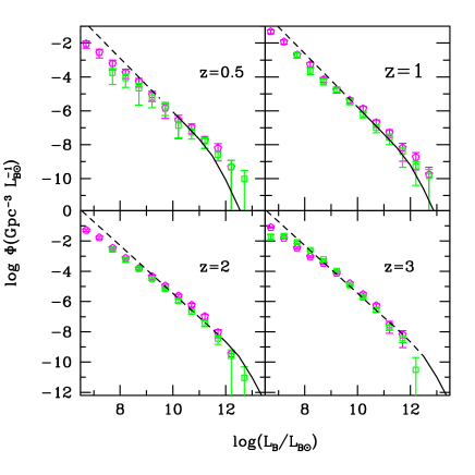
Figure 1: Luminosity function of AGN in the B-band corrected for absorption. Clockwise: z=0.5, 1, 2, 3. Green squares show model I ($f_{\rm Edd}$=1), magenta pentagons model IIIa ($f_{\rm Edd}$ luminosity dependent). Solid lines : 2QZ/6QZ LF. The dashed lines show the extrapolation to faint magnitudes.

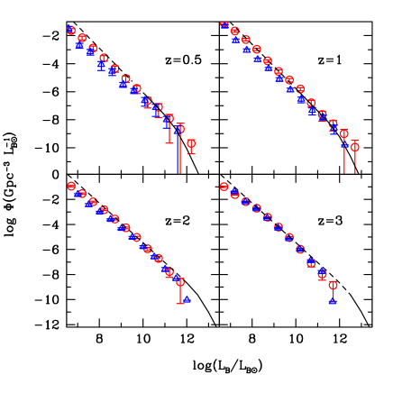
Figure 2: Luminosity function of AGN in the B-band corrected for absorption. Clockwise: z=0.5, 1, 2, 3. Blue triangles show model II ($f_{\rm Edd}$ redshift dependent), red circles model IIIb ($f_{\rm Edd}$ luminosity dependent).

The OLF is known to be a biased tracer of the accretion history of MBHs, missing the vast majority of Type II objectes. Moreover it spans a smaller range in luminosity compared to the HXLF (Ueda et al., 2003).

When we compare the theoretical and observed HXLFs of unabsorbed AGN (Figures 3 and 4), large differences at the faint end become apparent. Model I largely underestimates the faint end at $z\la 1$, while at $z\ga 2$ it agrees very well in the luminosity range probed by current surveys. Model II underestimates the normalization of HXLF at all redshift, although the shape is satisfactorily matched. In model II accretion is simply not enough to grow black holes massive enough to account for the bright end of the HXLF. If the normalization is changed from, $f_{\rm Edd,0}=0.3$ to $f_{\rm Edd,0}=1$ (cfr. Lapi et al. 2006), the model fares much better at high-z (basically corresponding to model I at $z>2$), but incurs in the same issues of model I at lower-z.

Models IIIa and IIIb fare better in reproducing the low redshift HXLF, but predicts a large population of faint AGN at $z\ga 2$ and slightly underestimate the bright end at high redshift ($z>2$). We note here that our approach differs from that by Hopkins et al. (2005). The starting point of Hopkins et al. (2005) is the HXLF, from which they derive the quasar birth rate, and consequently the OLF and other diagnostics. Our approach instead follows the evolutionary path of MBHs and AGN, that is the population evolves self-consistently along the cosmic epochs, according to the accretion properties stated in §2. The HXLF becomes therefore a constraint, rather than an input of the model as in Hopkins et al. (2005).

We have investigated the impact of the initial conditions, by applying model IIIa to a scenario in which seeds are much more massive, as in Koushiappas et al. (2004). The resulting luminosity functions are negligibly different with respect to the corresponding models assuming smaller seeds. This is because observable properties are mainly determined by the accretion history rather than by the initial conditions. Differences arise only at luminosity around $10^{42}$ erg s^-1, as a bump at $10^{42}$ erg s^-1, where the MBHs with a mass around that of the initial seeds are clustered, and a sharp decrease faint-ward of $10^{42}$ erg s^-1.

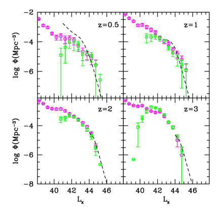
Figure 3: Luminosity function of AGN in the hard X-ray band [2-10 Kev]. Symbols as in Figure 1. The dashed lines show the Ueda et al. (2003) HXLF in the observationally constrained luminosity range.

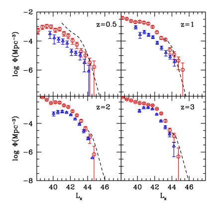
Figure 4: Luminosity function of AGN in the hard X-ray band [2-10 Kev]. Symbols as in Figure 2. The dashed lines show the Ueda et al. (2003) HXLF in the observationally constrained luminosity range.

4 Faint X-ray counts

The luminosity functions (OLF and HXLF) are the most sophisticated analysis of the evolution of AGN as a function of luminosity and redshift. On the other hand the available surveys do not probe yet the extreme faint end where theoretical models mostly differ, except at very low redshift. Figures 3 and 4 show that theoretical models predictions, at $z>0.5$ branch off at luminosities not yet sampled by the HXLF. Number counts are the results of integrating over intrinsic luminosity and distance. Number counts are a weaker test than the luminosity function, as AGN with a wide range of intrinsic luminosities are included at each flux. Nevertheless, they are the most direct probe of the AGN population. They are independent of cosmology, allow to probe further the faint population, where the HXLF is still prohibitive because of spectroscopic flux limits. We therefore compute the expected X-ray counts for the same AGN population that we used to determine the luminosity functions and compare the model results to the most recent determinations of X-ray counts and their redshift distribution.

4.1 Basic Equations

The number of sources (per unit solid angle) seen in the flux range $S$, $S+dS$ by an observer located at $z_{0}$, is

$$\frac{dN}{d\Omega dS}(z_{0},S)=\int^{\infty}_{z_{0}}\left(\frac{dV_{c}}{dzd\Omega}\right)n_{c}(z,S)\,dz,$$ (7)

where $dV_{c}/dzd\Omega$ is the comoving volume element per unit redshift per unit solid angle, and $n_{c}(z,S)$ is the comoving density of sources at redshift $z$, with observed flux in the range $[S,S+dS]$. The integrated flux of a source observed at $z_{0}$ is given by

$$S=\frac{1}{4\pi\,d_{L}^{2}(z_{0},z)}\int_{\Delta\nu}\tilde{L}_{\nu}(M)d\nu,$$ (8)

where $\nu=\nu_{0}(1+z)/(1+z_{0})$, $d_{L}(z_{0},z)$ is the luminosity distance between redshift $z_{0}$ and $z$, $\tilde{L}_{\nu}(M)$ is the specific luminosity averaged over the source lifetime (assumed to be only a function of the BH mass, $M$), and $\Delta\nu$ is the rest-frame frequency bandwidth.

The background specific intensity $J_{\nu_{0}}(z_{0})$ observed at redshift $z_{0}$ at frequency $\nu_{0}$, is

$$J_{\nu_{0}}(z_{0})=\frac{(1+z_{0})^{3}}{4\pi}\int^{\infty}_{z_{0}}\epsilon_{\nu}(z)\frac{dl}{dz}dz,$$ (9)

where $dl/dz$ is the proper line element, and the comoving specific emissivity $\epsilon_{\nu}(z)$ is given by

$$\epsilon_{\nu}(t) = \int dM\,\,\int_{0}^{t}L_{\nu}(t-t^{\prime},M)\frac{dn_{c}}{dt^{\prime}dM}dt^{\prime}$$ (10)

$$\simeq \int dM\,\,\tau\tilde{L}_{\nu}(M)\frac{dn_{c}}{dtdM}.$$

The second approximated equality holds once we consider the source light curve averaged over the typical source lifetime $\tau$, assuming the formation rate of sources per unit mass as constant over such timescale.

4.2 Number counts

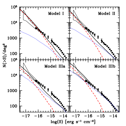
Figure 5: Predicted $\log(N)/\log(S)$ in the observed soft–X band [0.5–2 keV] for the different models. Dotted lines show the contribution of sources with $z<2$, whereas dashed lines the contribution of sources with $z>2$. Solid line is the sum of the two components. Points report data obtained with Chandra (dots; Moretti et al. 2003) and XMM (squares; Baldi et al. 2002), and the bow-tie indicates the result of the fluctuation analysis of the Chandra deep field (Bauer et al., 2004).

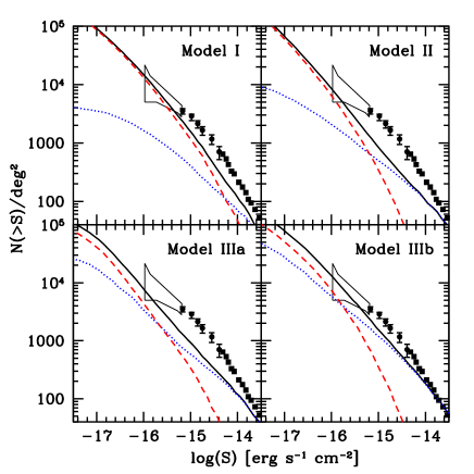
Figure 6: Predicted $\log(N)/\log(S)$ in the observed hard–X band [2–10 keV] for the different models. Lines and points are the same of Fig. 4.

We computed the number counts predicted by our different assumptions concerning the evolution of the Eddington–parameter along the cosmic history. The soft and hard X–ray logN/logS are shown in fig. 5 and fig. 6, respectively. The total counts (solid lines) are divided into the contribution of sources at $z<2$ (dotted lines), and $z>2$ (dashed lines). Model results are compared to a compilation of X–ray data from the Chandra (dots, Moretti et al. (2003)), and XMM (squares; Baldi et al. (2002)) deep field surveys. The bow–tie indicates results of the fluctuation analysis of the Chandra deep field (Bauer et al., 2004).

Model I fails to reproduce the slope of the observed logN/logS, falling short in the number of bright objects, and slightly overpredicting faint AGN. Moreover, the counts are dominated by high redshift sources for fluxes below $\log S<-14.6$. In Model II, the redshift distribution of AGN is somewhat pushed towards lower redshift, because of the relatively longer accretion time involved. The model underpredicts the counts both in the soft and hard X–ray bands, as BHs do not have enough time to grow. Model IIIa matches well the observed logN/logS in the soft band, but underpredicts the counts in the hard band. Finally, Model IIIb gives a reasonable good description in both bands, though it slightly overpredicts counts at very faint fluxes. AGN number counts are dominated, in the entire observed flux range, by low redshift objects, the contribution of sources at $z>2$ becoming significant only at fluxes as faint as the limits of the more recent surveys.

4.3 Redshift distribution of X–ray selected AGN

Aiming at constraining further the 4 different models employed, we compare the predicted redshift distributions to the results of the Serendipitous Extragalactic X-ray Source Identification (SEXSI) program, a survey designed to resolve a large fraction of the 2–10 keV cosmic X–ray background (Eckart et al., 2006). The survey covers 1 deg² for fluxes $>1\times 10^{-14}\;\mbox{erg s${}^{-1}$ cm${}^{-2}$}$, and 2 deg² for fluxes $>3\times 10^{-14}\;\mbox{erg s${}^{-1}$ cm${}^{-2}$}$. Given the large survey area, the SEXSI program minimizes the effects of cosmic variance. The catalog contains a total of 477 spectra, among which 438 have redshift and optical identification (Eckart et al., 2006). The Type I AGN redshift distribution of the SEXSI program and of our selected models are shown in fig. 7. Note that we splitted the original SEXSI data in order to match our definition of Type I/Type II sources. Moreover, we have convolved the predicted number counts with the sky coverage of the survey for different flux limits (Harrison et al., 2003).

Model I fails completely to reproduce the observed redshift distribution. In particular, the model largely underestimates the number of sources at $z<1.5$: the distribution peaks at redshift higher than observed. A better match to data is achieved by Model II. The general shape of the distribution is reproduced, although the model largely underestimates the total number of sources, as already pointed out. Model IIIa and IIIb are in reasonable agreement with the data. Model IIIa falls short to the data at $z<1$, while Model IIIb overpredicts the number of sources observed in the range $0.5<z<1.5$. In conclusion, the best agreement with the observed logN/logS, and with the redshift distribution of sources is found assuming a luminosity dependent Eddington rate (Hopkins et al., 2005).

We also tested that, in a model in which BH seeds are more massive, as in Koushiappas et al. (2004), the resulting $\log N/\log S$ and redshift distribution do not differ significantly with respect to models with earlier, smaller seeds. In conclusions, different formation scenarios for seed BHs are difficult to discriminate on the basis of available X–ray deep field surveys.

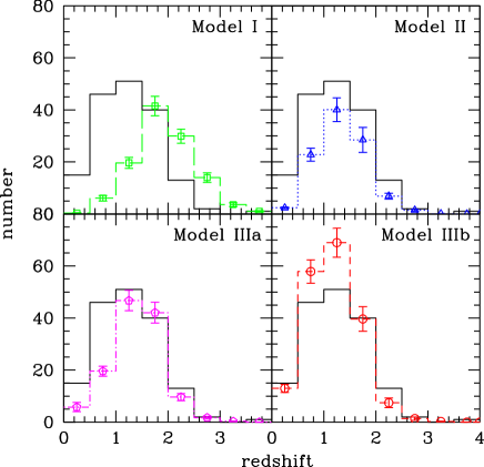
Figure 7: Distribution of Type I AGN as function of redshift for different models (points) compared to the result of Eckart et al. (2005; solid line) from the SEXSI program. In order to compare our results to the observed distribution, we have convolved the predicted number counts with the sky coverage of the survey at different flux limits (Harrison et al., 2003), and we have split the data so to match our definition of Type I/Type II sources.

4.4 Unresolved X–ray Background

According to Moretti et al. (2003), the intensity of the total X–ray background (XRB) is $7.53\pm 0.35\times 10^{-12}$ and $2.02\pm 0.11\times 10^{-11}\;\mbox{erg s${}^{-1}$ cm${}^{-2}$ deg${}^{-2}$}$ in the 0.5–2 keV, and 2–10 keV energy bands, respectively. A large fraction, $\simeq 94$%, of the soft XRB (SXRB) has been attributed to sources with fluxes exceeding $2.4\times 10^{-17}\;\mbox{erg s${}^{-1}$ cm${}^{-2}$}$, while $\sim 89$% of the hard XRB (HXRB) is resolved into sources whose flux is $\geq 2.1\times 10^{-16}\;\mbox{erg s${}^{-1}$ cm${}^{-2}$}$ (Moretti et al. 2003). More recently, Hickox & Markevitch (2006) estimated the unaccounted fraction of the XRB due to extragalactic unresolved sources as $1.77\pm 0.31\times 10^{-12}\;\mbox{erg s${}^{-1}$ cm${}^{-2}$ deg${}^{-2}$}$ in the soft X–ray energy band (0.5–2 keV) and $3.4\pm 1.7\times 10^{-12}\;\mbox{erg s${}^{-1}$ cm${}^{-2}$ deg${}^{-2}$}$ in the hard X–ray energy band (2–8 keV).

Using our different models, we compute the contribution to the unresolved XRB due to faint AGN lying below sensitivity limits of current X–ray surveys. The cumulative contribution from sources with flux above a given threshold is shown in Fig. 8, where it is compared to the recent estimate of Hickox & Markevitch (2005; shaded area). Different line styles refer to different models: Model I (long-dashed line), Model II (dotted line), Model IIIa (dot-dashed line), and Model IIIb (short-dashed line). The unresolved SXRB and HXRB are shown in the top and bottom panel, respectively. Although significant differences (within a factor of $\simeq 2$) are found between different models, all predict a contribution to the unresolved XRB consistent with available limits. Note that all models can account for the whole unresolved HXRB, while they give at most 50% of the unresolved SXRB. Our results imply the existence of a further population of faint X–ray sources in the soft band. Indeed, Salvaterra et al. (2006) have found that a significant contribution to the unresolved XRB may come from accreting BHs at very high redshift ($z>6$), a redshift range not considered here. By means of a dedicated model of the SMBH assembly at early times, consistent with the SDSS OLF at $z=6$ and with ultra–deep X–ray constraints, they found that the contribution to the SXRB of very high redshift, undetected AGN could be as high as $\sim 0.4\times 10^{-12}\;\mbox{erg s${}^{-1}$ cm${}^{-2}$ deg${}^{-2}$}$, providing the residual unresolved flux. The contribution of such population to the HXRB is still consistent with the available limits, being only $\sim 0.9\times 10^{-12}\;\mbox{erg s${}^{-1}$ cm${}^{-2}$ deg${}^{-2}$}$.

Figure 8: Predicted cumulative contribution to the unresolved XRB from different models as function of the X–ray flux. Different lines refer to different model: Model I (long-dashed line), Model II (dotted line), Model IIIa (dot-dashed line), and Model IIIb (short-dashed line). The shaded area show the measured unaccounted background as reported by Hickox & Markevitch (2005). Top panel: unaccounted XRB in the observed soft–X band [0.5-2 keV]. Bottom panel: unaccounted XRB in the observed hard–X band [2–8 keV].

5 Discussion

We have attempted in this paper to place constraints on the global accretion properties of the MBH population at $z<3$. We consider the full cosmological evolution of MBH embedded in their host halos, rather than adopting an empirical approach which takes as a starting point the observed LF in a given band in order to explain the properties of AGN in other bands. We focus here on the strength of accretion, parameterizing the accretion rate as a function of the Eddington rate, $f_{\rm Edd}$. We show that simple models which assume $f_{\rm Edd}=1$ (model I), although highly idealized, still are able to explain satisfactorily the growth of MBH, as traced by the OLF, in a large redshift range, as claimed previously by various investigations. Even at low redshift, where hierarchical models start to fail in their predictions, the OLF is very well reproduced. The HXLF probes fainter sources than the OLF, and the simplistic model I is shown to provide a poor match with the HXLF at $z<1$. A decreasing average Eddington ratio (Shankar et al., 2004, model II) provides a better agreement with the shape of the HXLF, but underestimates the normalization, as there is not enough time to grow high mass MBHs if the Eddington ratio is not large at $z>3$. A model (model III) with an Eddington ratio depending on luminosity (Hopkins et al., 2005; Shankar et al., 2004) seems to be the best match at low redshift. The difference among the models is magnified when the faint X-ray counts, and in particular their redshift distribution, are calculated. Model I has a strictly hierarchical growth of MBHs, and moreover, a univocal relationship between MBH mass and AGN luminosity. Model II allows massive black holes at low redshift to shine at lower luminosity, as the accretion rate, in units of the Eddington one, decreases with time. A rigid redshift dependence, however, creates two problems: first, subEddington accretion at $z>3$ implies a much slower growth for high redshift AGN, thus causing an underestimate of the LFs normalization at all the considered redshifts. Second, the evolution of the Eddington rate is not fast enough, at $z<3$, to account for the faint end of the LFs, in particular the HLF. The accretion rates, and Eddington ratios, predicted by simulations are here embedded into a cosmological framework (models IIIa and IIIb). The resulting AGN population provides a satisfactory match with the OLF, HXLF and faint X-ray counts at low redshift, while sources at high redshift are more problematic. The low accretion rates predicted by simulations imply very long growth timescales for black holes, and therefore underestimate the occurrence of bright quasars powered by billion solar masses black holes at high redshift ($z>2$).

It is not clear, however, if the accretion rate found in simulations, which relates to model III, i.e., strongly subEddington for low-luminosity sources (and therefore in all cases for small MBHs) indeed applies at very high-redshift. The simulations on which Hopkins et al. (2005) model is based assume mergers between ”normal” galaxies. How ”normal” are galaxies at $z>3$? It might indeed be possible that the conditions in pre-galactic structures at high-redshift (e.g., the disturbed morphological state of galaxies) cannot be studied with simulations of mergers of evolved discs and bulges, but would require different initial conditions for the merging galaxies. Future deep surveys can help us distinguish between various models in the high redshift Universe (see Figure 3), and can probably locate the time, if any, for a transition between messy mergers with on average efficient accretion onto the MBHs, and standard galactic mergers, predicting long periods of inefficient accretion.

Finally, we computed the contribution to the XRB of faint AGN lying below the sensitivity limits of current X–ray surveys. We found that all model predict a contribution to the unresolved XRB consistent with the available limits, accounting for the whole unresolved XRB in the 2–8 keV band and for $\sim 50$% in the 0.5–2 keV. The residual background intensity in the soft band may be provided by AGN shining at $z\ga 6$ (Salvaterra et al. 2006).

6 Acknowledgments

We would like to thank Dave Alexander for interesting discussions and helpful comments. This research was supported in part by the National Science Foundation under Grant No. PHY99-07949. NSF-KITP-06-88 pre-print.

References

- Aller & Richstone (2002) Aller M. C., Richstone D., 2002, AJ, 124, 3035
- Baldi et al. (2002) Baldi A., Molendi S., Comastri A., Fiore F., Matt G., Vignali C., 2002, ApJ, 564, 190
- Bauer et al. (2004) Bauer F. E., Alexander D. M., Brandt W. N., Schneider D. P., Treister E., Hornschemeier A. E., Garmire G. P., 2004, AJ, 128, 2048
- Cattaneo et al. (1999) Cattaneo A., Haehnelt M. G., Rees M. J., 1999, MNRAS, 308, 77
- Cavaliere & Vittorini (2000) Cavaliere A., Vittorini V., 2000, ApJ, 543, 599
- Croom et al. (2004) Croom S. M., Smith R. J., Boyle B. J., Shanks T., Miller L., Outram P. J., Loaring N. S., 2004, MNRAS, 349, 1397
- Di Matteo et al. (2005) Di Matteo T., Springel V., Hernquist L., 2005, Nat, 433, 604
- Eckart et al. (2006) Eckart M. E., Stern D., Helfand D. J., Harrison F. A., Mao P. H., Yost S. A., 2006, ApJS, 165, 19
- Ferrarese & Merritt (2000) Ferrarese L., Merritt D., 2000, ApJ, 539, L9
- Fiore et al. (2003) Fiore F., Brusa M., Cocchia F., Baldi A., Carangelo N., Ciliegi P., Comastri A., La Franca F., Maiolino R., Matt G., Molendi S., Mignoli M., Perola G. C., Severgnini P., Vignali C., 2003, A&A, 409, 79
- Gammie et al. (2004) Gammie C. F., Shapiro S. L., McKinney J. C., 2004, ApJ, 602, 312
- Gebhardt et al. (2000) Gebhardt K., et al., 2000, ApJ, 539, L13
- Granato et al. (2004) Granato G. L., De Zotti G., Silva L., Bressan A., Danese L., 2004, ApJ, 600, 580
- Haehnelt & Rees (1993) Haehnelt M. G., Rees M. J., 1993, MNRAS, 263, 168
- Haiman & Menou (2000) Haiman Z., Menou K., 2000, ApJ, 531, 42
- Harrison et al. (2003) Harrison F. A., Eckart M. E., Mao P. H., Helfand D. J., Stern D., 2003, ApJ, 596, 944
- Hatziminaoglou et al. (2001) Hatziminaoglou E., Siemiginowska A., Elvis M., 2001, ApJ, 547, 90
- Hickox & Markevitch (2006) Hickox R. C., Markevitch M., 2006, ApJ, 645, 95
- Hopkins et al. (2005) Hopkins P. F., Hernquist L., Cox T. J., Di Matteo T., Robertson B., Springel V., 2005, ApJ, 632, 81
- Hopkins et al. (2006) Hopkins P. F., Hernquist L., Cox T. J., Di Matteo T., Robertson B., Springel V., 2006, ApJS, 163, 1
- Hopkins et al. (2005) Hopkins P. F., Hernquist L., Martini P., Cox T. J., Robertson B., Di Matteo T., Springel V., 2005, ApJ, 625, L71
- Hunt et al. (2004) Hunt M. P., Steidel C. C., Adelberger K. L., Shapley A. E., 2004, ApJ, 605, 625
- Kauffmann & Haehnelt (2000) Kauffmann G., Haehnelt M., 2000, MNRAS, 311, 576
- Koushiappas et al. (2004) Koushiappas S. M., Bullock J. S., Dekel A., 2004, MNRAS, 354, 292
- La Franca et al. (2005) La Franca F., et al., 2005, ApJ, 635, 864
- Lapi et al. (2006) Lapi A., Shankar F., Mao J., Granato G. L., Silva L., De Zotti G., Danese L., 2006, ArXiv Astrophysics e-prints
- Madau & Rees (2001) Madau P., Rees M. J., 2001, ApJ, 551, L27
- Magorrian et al. (1998) Magorrian J., et al., 1998, AJ, 115, 2285
- Marconi et al. (2004) Marconi A., Risaliti G., Gilli R., Hunt L. K., Maiolino R., Salvati M., 2004, MNRAS, 351, 169
- Marulli et al. (2006) Marulli F., Crociani D., Volonteri M., Branchini E., Moscardini L., 2006, MNRAS, 368, 1269
- Merloni (2004) Merloni A., 2004, MNRAS, 353, 1035
- Merloni et al. (2003) Merloni A., Heinz S., di Matteo T., 2003, MNRAS, 345, 1057
- Mihos & Hernquist (1994) Mihos J. C., Hernquist L., 1994, ApJ, 425, L13
- Mihos & Hernquist (1996) Mihos J. C., Hernquist L., 1996, ApJ, 464, 641
- Moretti et al. (2003) Moretti A., Campana S., Lazzati D., Tagliaferri G., 2003, ApJ, 588, 696
- Richards et al. (2005) Richards G. T., et al., 2005, MNRAS, 360, 839
- Sazonov et al. (2004) Sazonov S. Y., Ostriker J. P., Sunyaev R. A., 2004, MNRAS, 347, 144
- Shankar et al. (2004) Shankar F., Salucci P., Granato G. L., De Zotti G., Danese L., 2004, MNRAS, 354, 1020
- Springel et al. (2005) Springel V., et al., 2005, Nat, 435, 629
- Ueda et al. (2003) Ueda Y., Akiyama M., Ohta K., Miyaji T., 2003, ApJ, 598, 886
- Volonteri et al. (2003) Volonteri M., Haardt F., Madau P., 2003, ApJ, 582, 559
- Volonteri et al. (2003) Volonteri M., Madau P., Haardt F., 2003, ApJ, 593, 661
- Volonteri et al. (2005) Volonteri M., Madau P., Quataert E., Rees M. J., 2005, ApJ, 620, 69
- Volonteri & Rees (2006) Volonteri M., Rees M. J., 2006, ApJ, in press
- Wyithe & Loeb (2003) Wyithe J. S. B., Loeb A., 2003, ApJ, 595, 614