Physics of Strongly Magnetized Neutron Stars

Abstract

There has recently been growing evidence for the existence of neutron stars possessing magnetic fields with strengths that exceed the quantum critical field strength of $4.4\times 10^{13}$ G, at which the cyclotron energy equals the electron rest mass. Such evidence has been provided by new discoveries of radio pulsars having very high spin-down rates and by observations of bursting gamma-ray sources termed magnetars. This article will discuss the exotic physics of this high-field regime, where a new array of processes becomes possible and even dominant, and where familiar processes acquire unusual properties. We review the physical processes that are important in neutron star interiors and magnetospheres, including the behavior of free particles, atoms, molecules, plasma and condensed matter in strong magnetic fields, photon propagation in magnetized plasmas, free-particle radiative processes, the physics of neutron star interiors, and field evolution and decay mechanisms. Application of such processes in astrophysical source models, including rotation-powered pulsars, soft gamma-ray repeaters, anomalous X-ray pulsars and accreting X-ray pulsars will also be discussed. Throughout this review, we will highlight the observational signatures of high magnetic field processes, as well as the theoretical issues that remain to be understood.

1 Introduction

Since their theoretical conception by Baade & Zwicky (1934) neutron stars have been fascinating celestial objects, both for study of their exotic environments and for their important place in stellar evolution. Among the first signals to be detected from neutron stars came from radio pulsars (Hewish et al. 1968), spinning many times per second, distinguishing themselves from the background of interplanetary scintillation signals by their extremely regular pulsations. Pulsars were also soon discovered to be spinning down, their periods increasing also very regularly. The rotating magnetic-dipole model (Pacini 1967, Gold 1968, Ostriker & Gunn 1969), in which the pulsar loses rotational energy through magnetic dipole radiation, was dramatically confirmed with the discovery that the spin-down power predicted for the Crab pulsar was a nearly perfect energetic match with the radiation of its synchrotron nebula. The rotating dipole model also accounts for the observed rate of spin-down of the Crab and other pulsars, with required surface magnetic fields in the range of $10^{11}-10^{13}$ Gauss for the first detected pulsars. This range has since significantly broadened, first with the discovery of a class of pulsars having periods of several milliseconds (Backer et al. 1982), believed to have been spun-up by accretion torques of a binary companion (Alpar et al. 1982), and much lower surface magnetic fields in the range of $10^{8}-10^{10}$ Gauss. Recent surveys have also discovered pulsars with very high period derivatives (e.g. Morris et al. 2002, McLaughlin et al. 2003) that imply surface fields up to around $10^{14}$ Gauss.

Another class of neutron stars was discovered at X-ray and $\gamma$-ray energies and may possess even stronger surface magnetic fields. Such stars are now referred to as magnetars (Duncan & Thompson 1992), since they most probably derive their power from their magnetic fields rather than from spin-down energy loss (see Woods & Thompson 2005). Within the magnetar class there are two types of sources that were originally thought to be very different objects, although they are now believed to be closely related. The Anomalous X-Ray Pulsars (AXPs) were discovered as pulsating X-ray sources in the early 1980s and were thought at first to be an unusual type of accreting X-ray pulsar, from which the name is derived. The AXPs have periods in a relatively narrow range of 5 - 11 s, are observed to be spinning down with large period derivatives (Vasisht & Gotthelf 1997) and have no detectable companions or accretion disks that would be required to support the accretion hypothesis. Interpretation of their period derivatives as magnetic dipole spin down imply magnetic fields in the range $10^{14}-10^{15}$ Gauss. But such high fields were not widely accepted initially, since their detected X-ray luminosities of around $10^{35}\,\rm erg\,s^{-1}$ exceed their spin-down luminosities by several orders of magnitude. It was only by connection to another subclass of magnetar, the Soft Gamma-Ray Repeaters (SGRs), that the extremely high magnetic fields of AXPs were adopted. SGRs were discovered as transient sources that undergo repeated soft $\gamma$-ray bursts, usually in widely separated episodes. They undergo both repeated smaller bursting of subsecond duration as well as much more luminous superflares, lasting hundreds of seconds, which so far have not repeated in any single source but may be repeating on much longer timescales. It was not until some twenty years after their discovery that their quiescent X-ray pulsations were detected and also very high period derivatives (Kouveliotou et al. 1998), both with a range of values very similar to those of AXPs. Recently, bursts resembling the smaller bursts of SGRs were seen from several AXPs (Kaspi et al. 2003), making it likely that SGRs and AXPs are two variations of the same type of object (Thompson & Duncan 1993), very strongly magnetized, isolated neutron stars possibly powered by magnetic field decay.

The periods and period derivatives of the various types of isolated pulsars are shown in the $P$-$\dot{P}$ diagram of Figure 1. Assuming that the spindown torque is due to magnetic dipole radiation, two quantities can be defined from the measured $P$ and $\dot{P}$ for each pulsar: (1) Characteristic age $P/(2\dot{P})$: From $\dot{\Omega}\propto-\Omega^{3}$ (where $\Omega=2\pi/P$), the age of the pulsar is found to be $T=(P/2\dot{P})[1-(P/P_{i})^{2}]$, where $P_{i}$ is the pulsar’s initial spin period. (2) Surface dipole magnetic field:

$$B_{s}=\left({\frac{{3Ic^{3}P\dot{P}}}{{2\pi^{2}R^{6}}}}\right)^{1/2}\simeq 2\times 10^{12}{\rm G}\,(P\dot{P}_{15})^{1/2},$$ (1)

where $\dot{P}_{15}\equiv\dot{P}/(10^{-15}\,\rm s\,s^{-1})$ (and $P$ is in units of second), and and $I$ ($\simeq 10^{45}$ g cm² and $R$ ($\simeq 10^{6}$ cm) are the neutron star moment of inertia and radius. There are presently around 1600 spin-powered radio pulsars known, with periods from $1.5$ ms - 8 s (Manchester 2004). Some fraction of these pulse at other wavelengths, including about 10 in $\gamma$-rays and about 30 in X-rays. The magnetars, eight AXPs and four SGRs, occupy the upper right-hand corner of the diagram and curiously overlap somewhat with the region occupied by the high-field radio pulsars. However, the two types of objects display very different observational behavior. The high-field radio pulsars have very weak or non-detectable X-ray emission and do not burst (e.g. Kaspi & McLaughlin 2005), while the magnetars have no detectable radio pulsations, with the exception of the recent detection of radio pulsations in the transient AXP XTE J1810-197 (Camilo et al. 2006). The intrinsic property that actually distinguishes magnetars from radio pulsars is presently not understood.

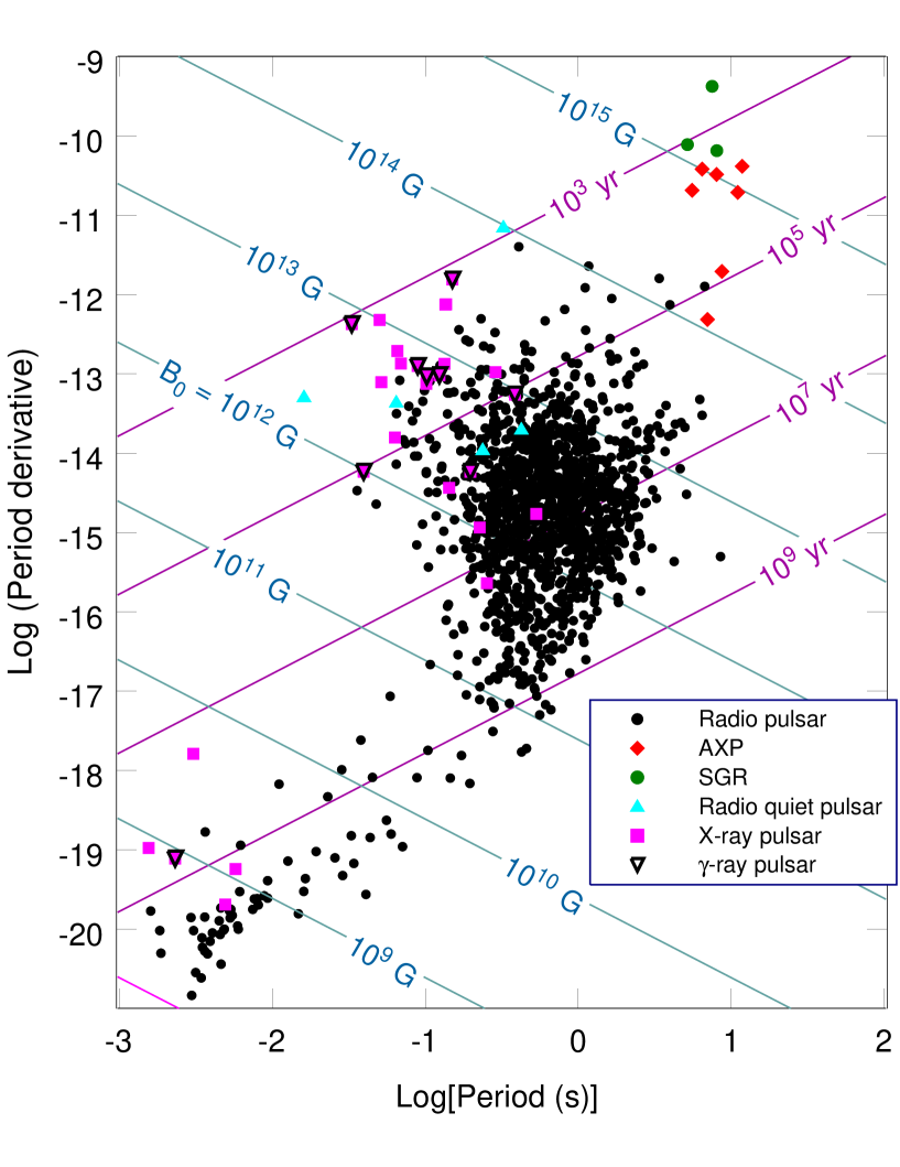
Figure 1: Plot of period vs. period derivative for the presently known rotation-powered pulsars and magnetars. Lines of constant characteristic age, $P/2\dot{P}$, and surface dipole field (see Eqn [1]) are superposed.

A third class of strongly magnetized neutron stars are the accreting X-ray pulsars (Parmar 1994). These sources are members of binary systems with high-mass companions that either have strong stellar winds or overflow their Roche lobes, transferring material to the neutron star. Inside an Alfven surface where the pressure of the accretion flow equals the neutron star magnetic field pressure, the accreting material is funneled along the magnetic field to the poles. The heated accretion flow then radiates from hot spots that rotate with the star, thereby producing pulsations. However, since accretion torques dominate the period derivative evolution, the surface magnetic fields of X-ray pulsars cannot be determined using the rotating dipole model, as they are for the rotation-powered pulsars and magnetars. Instead, magnetic fields of these objects have been measured from the energies of the cyclotron resonant scattering features (CRSFs) that appear in their spectra (see Orlandini & dal Fiume 2001, for review), since the fundamental occurs at the electron cyclotron energy, $E_{ce}=\hbar eB/(m_{e}c)=11.58\,(B/10^{12}\,{\rm G})$ keV. Table 1 lists the X-ray pulsars, the energies of CRSFs that have been detected in their spectra and the inferred magnetic field strengths. In most cases, the measured magnetic fields range from $1-5\times 10^{12}$ Gauss, with the highest fields being around $4\times 10^{12}$Gauss. The formation of such line features will be discussed in section 11.

Table 1: X-Ray Pulsars with Cyclotron Resonant Scattering Features^a

Source	Energy (keV)b	B ($10^{12}$ Gauss)c
4U 0115+63	12 (4)	1.0
4U 1907+09	18 (1)	1.6
4U 1538-52	20	1.7
Vela X-1	25 (1)	2.2
V 0332+53	27 (2)	2.3
Cep X-4	28	2.4
Cen X-3	28.5	2.5
X Per	29	2.5
XTE J1946+274	36	3.1
MX0656-072	36	3.1
4U 1626-67	37	3.2
GX 301-2	37	3.2
Her X-1	41	3.5
A 0535+26	47d (2)	4.1

^a Data is from Heindl et al. (2004).

^b Numbers in parentheses are the number of cyclotron harmonics detected.

^c Magnetic field strength for viewing angle along field direction.

^d Kretschmar et al. (2005)

Clearly, there is a broad range of astrophysical sources in which the magnetic fields approach and exceed the quantum critical field strength, $B_{Q}\equiv m_{e}^{2}c^{3}/(e\hbar)=4.414\times 10^{13}$ G, at which the cyclotron energy equals the electron rest mass. In this regime, the magnetic field profoundly affects physical processes and introduces additional processes that do not take place in field-free environments. From a physics point of view, strongly magnetized neutron stars provide the only environment in which to measure and test these effects. From an astrophysics point of view, it is necessary to investigate the physics of strong magnetic fields in order to effectively model and understand the nature of the sources. This article will attempt to address both points of view by providing a review of the basic physical processes important in neutron star interiors and magnetospheres, as well as a review of the source models in which these processes play a critical role.

We begin with a description of a free electron in a magnetic field in both classical and quantum regimes. Subsequent sections then discuss and review current understanding of the behavior of matter, atoms, molecules and plasma, in strong magnetic fields, photon propagation in magnetized plasmas, free-particle radiative processes, the physics of neutron star interiors, and field evolution and decay mechanisms. Then we will review models for magnetized atmospheres, non-thermal radiation from rotation-powered pulsars, burst and quiescent radiation from SGRs and AXPs, and emission from accreting X-ray pulsars. Other useful books and reviews on strongly magnetized neutron stars include Meszaros (1992), Duncan (2000), Lai (2001) and Harding (2003). A complimentary work concentrating on stellar magnetism in general is the book by Mestel (1999).

2 Electrons in Strong Magnetic Fields

The quantum mechanics of a charged particle in a magnetic field is presented in many texts (e.g., Landau & Lifshitz 1977; Sokolov & Ternov 1968; Mészáros 1992). Here we summarize the basics needed for our later discussion.

Consider first the nonrelativistic motion of a particle (charge $e_{i}$ and mass $m_{i}$) in a uniform magnetic field ${\bf B}$ (assumed to be along the $z$-axis). In classical physics, the particle gyrates in a circular orbit with radius and (angular) frequency given by

$$\rho={m_{i}cv_{\perp}\over|e_{i}|B},\quad\omega_{c}={|e_{i}|B\over m_{i}c},$$ (2)

where $v_{\perp}$ is the velocity perpendicular to the magnetic field. In non-relativistic quantum mechanics, the kinetic energy of the transverse motion is quantized in Landau levels

$$E_{\perp}={1\over 2}m_{i}{\bf v}_{\perp}^{2}={1\over 2m_{i}}{\bf\Pi}_{\perp}^{2}\rightarrow\left(n_{L}+{1\over 2}\right)\hbar\omega_{c},\qquad n_{L}=0,1,2,\cdots$$ (3)

where ${\bf\Pi}={\bf p}-(e_{i}/c){\bf A}=m_{i}{\bf v}$ is the mechanical momentum, ${\bf p}=-i\hbar{\bf\nabla}$ is the canonical momentum, and ${\bf A}$ is the vector potential of the magnetic field.

For an electron ($m_{i}\rightarrow m_{e},~{}e_{i}\rightarrow-e$), the basic energy quantum is the cyclotron energy

$$E_{ce}=\hbar\omega_{ce}=\hbar{eB\over m_{e}c}=11.577\,B_{12}~{}{\rm keV},$$ (4)

where $B_{12}=B/(10^{12}\,{\rm G})$ is the magnetic field strength in units of $10^{12}$ Gauss. Including the kinetic energy associated with the $z$-momentum ($p_{z}$) and the spin energy, $E_{\sigma_{z}}=e\hbar/(2m_{e}c){\mbox{\boldmath$\sigma$}}\cdot{\bf B}=\hbar\omega_{ce}\sigma_{z}/2$ (with $\sigma_{z}=\pm 1$), the total electron energy can be written as

$$E_{n}=n\hbar\omega_{ce}+{p_{z}^{2}\over 2m_{e}},$$ (5)

where the index $n=n_{L}+(1+\sigma_{z})/2=0,1,\cdots$. Clearly, for the ground Landau level ($n=0$), the spin degeneracy is one ($\sigma_{z}=-1$); for excited levels, the spin degeneracy is two ($\sigma_{z}=\pm 1$).

Apart from the spin degeneracy, the Landau level associated with Eq. (3) is degenerate by itself, reflecting the fact that the energy is independent of the location of the guiding center of the gyration. To count the degeneracy, it is useful to define the pseudomomentum (or the generalized momentum)

$${\bf K}={\bf\Pi}+(e_{i}/c){\bf B}\times{\bf r}.$$ (6)

That ${\bf K}$ is a constant of motion (i.e., it commutes with the Hamiltonian) can be easily seen from the classical equation of motion for the particle, $d{\bf\Pi}/dt=(e_{i}/c)(d{\bf r}/dt)\times{\bf B}$. The parallel component $K_{z}$ is simply the linear momentum $p_{z}$, while the perpendicular component ${\bf K}_{\perp}$ is related to the position vector ${\bf R}_{c}$ of the guiding center by

$${\bf R}_{c}={c{\bf K}_{\perp}\times{\bf B}\over e_{i}B^{2}}={c\over e_{i}B}{\bf\Pi}_{\perp}\times\hat{\bf B}+{\bf r}_{\perp},$$ (7)

($\hat{\bf B}$ is the unit vector along ${\bf B}$). From Eqs. (3) and (7), we see that classical radius of gyration, $\rho=|{\bf r}_{\perp}-{\bf R}_{c}|$ (see eq. [2]), is quantized according to

$$|{\bf r}_{\perp}-{\bf R}_{c}|={c\over|e_{i}|B}|{\bf\Pi}_{\perp}|\rightarrow(2n_{L}+1)^{1/2}\hat{\rho},$$ (8)

where

$$\hat{\rho}=\left({\hbar c\over|e_{i}|B}\right)^{1/2}$$ (9)

is the cyclotron radius (or the magnetic length). Since the two components of ${\bf K}_{\perp}$ do not commute, $[K_{x},K_{y}]=-i\hbar(e_{i}/c)B$, only one of the components can be diagonalized for stationary states. This means that the guiding center of the particle can not be specified. If we use $K_{x}$ to classify the states, then the wavefunction has form $e^{iK_{x}x/\hbar}\phi(y)$ (Landau & Lifshitz 1977), where the function $\phi(y)$ is centered at $y_{c}=-cK_{x}/(e_{i}B)$ [see Eq. (7)]. The Landau degeneracy in an area ${\cal A}_{g}=L_{g}^{2}$ is thus given by

$${L_{g}\over h}\int\!dK_{x}={L_{g}\over h}|K_{x,g}|={\cal A}_{g}{|e_{i}|B\over hc}={{\cal A}_{g}\over 2\pi\hat{\rho}^{2}},$$ (10)

where we have used $K_{x,g}=-e_{i}BL_{g}/c$. Alternatively, if we choose to diagonalize $K_{\perp}^{2}=K_{x}^{2}+K_{y}^{2}$, we obtain the Landau wavefunction $W_{nm}({\bf r}_{\perp})$ in cylindrical coordinates (Landau & Lifshitz 1977), where $m$ is the “orbital” quantum number (denoted by $s$ or $-s$ in some references). For the ground Landau level, this is (for $e_{i}=-e$)

$$W_{0m}({\bf r}_{\perp})\equiv W_{m}(\rho,\phi)={1\over(2\pi m!)^{1/2}\hat{\rho}}\left({\rho\over\sqrt{2}\hat{\rho}}\right)^{m}\exp\left({\rho^{2}\over 4\hat{\rho}^{2}}\right)\exp(-im\phi),$$ (11)

where the normalization $\int d^{2}{\bf r}_{\perp}\,|W_{m}|^{2}=1$ is adopted. The (transverse) distance of the particle’s guiding center from the origin of the coordinates is given by

$$|{\bf R}_{c}|\rightarrow\rho_{m}=(2m+1)^{1/2}\hat{\rho},~{}~{}~{}~{}~{}m=0,1,2,\cdots$$ (12)

The corresponding value of $K_{\perp}$ is $K_{\perp}^{2}=(\hbar|e_{i}|B/c)(2m+1)$. Note that $K_{\perp}^{2}$ assumes discrete values since $m$ is required to be an integer in order for the wavefunction to be single-valued. The degeneracy $m_{g}$ of the Landau level in an area ${\cal A}_{g}=\pi R_{g}^{2}$ is then determined by $\rho_{m_{g}}\simeq(2m_{g})^{1/2}\hat{\rho}=R_{g}$, which again yields $m_{g}={\cal A}_{g}|e_{i}|B/(hc)$ as in Eq. (10). Note that despite the similarity between Eqs. (12) and (8), their physical meanings are quite different: the circle $\rho=\rho_{m}$ does not correspond to any gyro-motion of the particle, and the energy is independent of $m$. Also note that $K_{\perp}^{2}$ is related to the $z$-projection of angular momentum $J_{z}$, as is evident from the $e^{-im\phi}$ factor in the cylindrical wavefunction [Eq. (11)]. In general, we have

$$J_{z}=xP_{y}-yP_{x}={1\over 2e_{i}B}({\bf K}_{\perp}^{2}-{\bf\Pi}_{\perp}^{2})=(m-n_{L}){|e_{i}|\over e_{i}},$$ (13)

where we have used ${\bf\Pi}_{\perp}^{2}=(\hbar|e_{i}|/c)B(2n_{L}+1)$.

For extremely strong magnetic fields such that $\hbar\omega_{ce}\mathrel{\raise 1.29167pt\hbox{$>$}\mkern-14.0mu\lower 2.58334pt\hbox{$\sim$}}m_{e}c^{2}$, or

$$B\mathrel{\raise 1.29167pt\hbox{$>$}\mkern-14.0mu\lower 2.58334pt\hbox{$\sim$}}B_{Q}={m_{e}^{2}c^{3}\over e\hbar}=4.414\times 10^{13}~{}{\rm G},$$ (14)

the transverse motion of the electron becomes relativistic. The transverse momentum is again quantized according to Eq. (3), i.e., ${\bf\Pi}_{\perp}^{2}\rightarrow\left(2n_{L}+1\right)\hbar eB/c$. By solving the Dirac Equation in a homogeneous magnetic field, we find that Eq. (5) for the energy of a free electron should be replaced by (e.g., Johnson & Lippmann 1949)

$$E_{n}=\left[c^{2}p_{z}^{2}+m_{e}^{2}c^{4}\left(1+2n{B\over B_{Q}}\right)\right]^{1/2}.$$ (15)

The shape of the Landau wavefunction in the relativistic theory is the same as in the nonrelativistic theory, as seen from the fact that $\hat{\rho}$ is independent of the particle mass (see Sokolov & Ternov 1968). Higher order corrections in $e^{2}$ to Eq. (15) have the form $(\alpha/4\pi)m_{e}c^{2}F(B/B_{Q})$, with $\alpha=1/37$ the fine structure constant, $F(\beta)=-\beta$, $\beta\equiv B/B_{Q}$, for $\beta\ll 1$ and $F(\beta)=\left[\ln(2\beta)-(\gamma_{E}+3/2)\right]^{2}+\cdots$ for $\beta\gg 1$, where $\gamma_{E}=0.5772$ is Euler’s constant (Schwinger 1988); these corrections are negligible.

Calculations based on electron wavefunctions that are solutions to the Dirac Equation in Cartesian and in cylindrical coordinates have both appeared in the literature. As is true for all quantum processes, the rates and cross sections depend on the choice of electron wavefunctions in a uniform magnetic field, which are dependent on spin state. The two most widely used relativistic wavefunctions are those of Johnson and Lippman (1949) and Sokolov & Ternov (ST) (1968). The Johnson and Lippman (JL) wavefunctions are derived in Cartesian coordinates and are eigenstates of the kinetic momentum operator $\pi=p+eA/c$. The Sokolov & Ternov (ST) wavefunctions, given for the ground state in Eqn (11), are derived in cylindrical coordinates and are eigenstates of the field parallel component, $\mu_{z}$, of the magnetic moment operator. Given the different spin dependence of the ST and JL eigenstates, one must use caution in making the appropriate choice when treating spin-dependent processes. Herold et al. (1982) and Melrose and Parle (1983) have noted that the ST eigenstates have desirable properties that the JL do not possess, such as being eigenfunctions of the Hamiltonian including radiation corrections, having symmetry between positron and electron states, and diagonalization of the self-energy shift operator. As found by Graziani (1993), the ST wavefunctions also diagonalize the Landau-Dirac operator and are the physically correct choices for spin-dependent treatments and in incorporating widths in the scattering cross section. Although the spin-averaged ST and JT cyclotron decay rates are equal, for example, the spin-dependent decay rates are not, except in the special case in which the initial momentum of the electron parallel to the magnetic field vanishes. An additional desirable property of the ST states is that spin-dependent states are preserved under Lorentz transformations while Lorentz boosts mix spin states of the JL wavefunctions.

3 Matter in Strong Magnetic Fields

When studying matter in magnetic fields, the natural (atomic) unit for the field strength, $B_{0}$, is set by equating the electron cyclotron energy $\hbar\omega_{ce}$ to the characteristic atomic energy $e^{2}/a_{0}=2\times 13.6$ eV (where $a_{0}$ is the Bohr radius), or equivalently by $\hat{\rho}=a_{0}$. Thus it is convenient to define a dimensionless magnetic field strength $b$ via

$$b\equiv{B\over B_{0}};\qquad B_{0}={m_{e}^{2}e^{3}c\over\hbar^{3}}=\alpha^{2}B_{Q}=2.3505\times 10^{9}\,{\rm G}$$ (16)

($\alpha=1/137$ is the fine structure constant). For $b\gg 1$, the cyclotron energy $\hbar\omega_{ce}$ is much larger than the typical Coulomb energy, so that the properties of atoms, molecules and condensed matter are qualitatively changed by the magnetic field. In such a strong field regime, the usual perturbative treatment of the magnetic effects (e.g., Zeeman splitting of atomic energy levels) does not apply (see Garstang 1977 for a review of atomic physics at $b\mathrel{\raise 1.29167pt\hbox{$<$}\mkern-14.0mu\lower 2.58334pt\hbox{$\sim$}}1$). Instead, the Coulomb forces act as a perturbation to the magnetic forces, and the electrons in an atom settle into the ground Landau level. Because of the extreme confinement ($\hat{\rho}\ll a_{0}$) of the electrons in the transverse direction (perpendicular to the field), the Coulomb force becomes much more effective in binding the electrons along the magnetic field direction. The atom attains a cylindrical structure. Moreover, it is possible for these elongated atoms to form molecular chains by covalent bonding along the field direction. Interactions between the linear chains can then lead to the formation of three-dimensional condensates.

Note that when studying bound states (atoms, molecules and condensed matter near zero pressure) in strong magnetic fields, it is adequate to use nonrelativistic quantum mechanics, even for $B\mathrel{\raise 1.29167pt\hbox{$>$}\mkern-14.0mu\lower 2.58334pt\hbox{$\sim$}}B_{Q}$. The nonrelativistic treatment of bound states is valid for two reasons: (i) For electrons in the ground Landau level, eq. (15) for the free electron energy reduces to $E\simeq m_{e}c^{2}+p_{z}^{2}/(2m_{e})$ for $p_{z}c\ll m_{e}c^{2}$; the electron remains nonrelativistic in the $z$-direction (along the field axis) as long as the binding energy $E_{B}$ is much less than $m_{e}c^{2}$; (ii) As mentioned before (§2), the shape of the Landau wavefunction in the relativistic theory is the same as in the nonrelativistic theory. Therefore, as long as $E_{B}/(m_{e}c^{2})\ll 1$, the relativistic effect on bound states is a small correction. For bulk matter under pressure, the relativistic correction becomes increasingly important as density increases (see §6).

Note that unless specified, the expressions in this section will be in atomic units (a.u.), where mass and length are expressed in units of the electron mass $m_{e}$ and the Bohr radius $a_{0}=0.529\times 10^{-8}$ cm, energy in units of $2~{}{\rm Ryd}=e^{2}/a_{0}=2\times 13.6$ eV, field strength in units of $B_{0}$ [Eq. (16)]. A previous (more detailed) review on this subject is Lai (2001), where more complete references can be found.

3.1 Hydrogen Atom

In a strong magnetic field with $b\gg 1$, the electron is confined to the ground Landau level (“adiabatic approximation”), and the Coulomb potential can be treated as a perturbation. Assuming infinite proton mass (see below), the energy spectrum of the H atom is specified by two quantum numbers, $(m,\nu)$, where $m$ measures the mean transverse separation [Eq. (12)] between the electron and the proton, while $\nu$ specifies the number of nodes in the $z$-wavefunction. There are two distinct types of states in the energy spectrum $E_{m\nu}$. The “tightly bound” states have no node in their $z$-wavefunctions ($\nu=0$). The transverse size of the atom in the $(m,0)$ state is $L_{\perp}\sim\rho_{m}=[(2m+1)/b]^{1/2}$. For $\rho_{m}\ll 1$, the atom is elongated with $L_{z}\gg L_{\perp}$. We can estimate the longitudinal size $L_{z}$ by minimizing the energy, $E\sim L_{z}^{-2}-L_{z}^{-1}\ln(L_{z}/L_{\perp})$ (where the first term is the kinetic energy and the second term is the Coulomb energy), giving

$$L_{z}\sim{1\over 2\ln(1/\rho_{m})}=\left(\ln{b\over 2m+1}\right)^{-1}.$$ (17)

The energy of the tightly bound state is then

$$E_{m0}\simeq-0.16A\,\left(\ln{b\over 2m+1}\right)^{2}\qquad({\rm for}~{}~{}2m+1\ll b).$$ (18)

Here the numerical prefactor comes from solving the Schrödinger equation. The coefficient $A$ in (18) is close to unity for the range of $b$ of interest ($1\ll b\mathrel{\raise 1.29167pt\hbox{$<$}\mkern-14.0mu\lower 2.58334pt\hbox{$\sim$}}10^{6}$) and varies slowly with $b$ and $m$ (e.g., $A\simeq 1.01-1.3$ for $m=0-5$ when $B_{12}=1$, and $A\simeq 1.02-1.04$ for $m=0-5$ when $B_{12}=10$. Note that $E_{m0}$ asymptotically approaches $-0.5\,\left[\ln{b/(2m+1)}\right]^{2}$ when $b\rightarrow\infty$). Obviously the ground-state binding energy $|E_{00}|$ (e.g., $160$ eV at $10^{12}$ G and $540$ eV at $10^{14}$ G) is much larger than the zero-field value (13.6 eV). For $\rho_{m}\mathrel{\raise 1.29167pt\hbox{$>$}\mkern-14.0mu\lower 2.58334pt\hbox{$\sim$}}1$, or $2m+1\mathrel{\raise 1.29167pt\hbox{$>$}\mkern-14.0mu\lower 2.58334pt\hbox{$\sim$}}b$ [but still $b\gg(2m+1)^{-1}$ so that the adiabatic approximation ($|E_{m0}|\ll b$) is valid], we have $L_{z}\sim\rho_{m}^{1/2}$, and the energy levels are approximated by

$$E_{m0}\simeq-0.6\,\left({b\over 2m+1}\right)^{1/2}\qquad[{\rm for}~{}~{}2m+1\mathrel{\raise 1.29167pt\hbox{$>$}\mkern-14.0mu\lower 2.58334pt\hbox{$\sim$}}b\gg(2m+1)^{-1}].$$ (19)

Again the prefactor 0.6 comes from solution of the Schrödinger equation. Numerical values of $E_{m0}$ for different $B$’s can be found, for example, in Ruder et al. (1994). Fitting formulae for $E_{m0}$ are given in Potekhin (1998) and in Ho et al. (2003).

Another type of states of the H atom has nodes in the $z$-wavefunctions ($\nu>0$). These states are “weakly bound”, and have energies (for $b\gg 1$) of order $E_{m\nu}\sim-\nu^{-2}$ Ry (see Lai 2001 and references therein; see also Potekhin 1998 for a comprehensive set of fitting formulae). The sizes of the wavefunctions are $\rho_{m}$ perpendicular to the field and $L_{z}\sim\nu^{2}a_{0}$ along the field.

This simple picture of the H energy levels is modified when a finite proton mass is taken into account. Even for a “stationary” H atom, the energy $E_{m\nu}$ should be replaced by $E_{m\nu}+m\hbar\omega_{cp}$, where $\hbar\omega_{cp}=\hbar eB/(m_{p}c)=6.3\,B_{12}$ eV is the proton cyclotron energy (e.g. Herold et al. 1981). The extra “proton recoil” energy $m\hbar\omega_{cp}$ becomes increasingly important with increasing $B$. Moreover, the effect of center-of-mass motion is non-trivial: When the atom moves perpendicular to the magnetic field, an electric field is induced in its rest frame and can significantly change the atomic structure, i.e., there is a strong coupling between the center-of-mass motion and the “internal” electron motion. It is easy to show that even including the Coulomb interaction, the total pseudomomentum,

$${\bf K}={\bf K}_{e}+{\bf K}_{p},$$ (20)

is a constant of motion. Moreover, all components of ${\bf K}$ commute with each other. Thus it is natural to separate the CM motion from the internal degrees of freedom using ${\bf K}$ as an explicit constant of motion. From Eq. (7), we find that the separation between the guiding centers of the electron and the proton is directly related to ${\bf K}_{\perp}$:

$${\bf R}_{K}={\bf R}_{ce}-{\bf R}_{cp}={c{\bf B}\times{\bf K}\over eB^{2}}.$$ (21)

For sufficiently small $K_{\perp}$, it is convenient to think of the effect of center-of-mass motion as the “motional Stark effect”, and the kinetic energy associated with the transverse motion is $K_{\perp}^{2}/(2M_{\perp m})$. Here the effective mass $M_{\perp m}$ depends on the energy levels, and increases with increasing $B$. For large transverse pseudomomentum $K_{\perp}$, the structure of the “moving” atom is qualitatively different from the stationary atom: The atom assumes a decentered configuration, with transverse electron-proton separation $\sim R_{K}$, and longitudinal separation $\sim R_{K}^{3/4}$, and its energy depends on $K_{\perp}$ as $-R_{K}^{-1}=-b/K_{\perp}$ rather than the usual $K_{\perp}^{2}$ dependence (see Lai 2001 and Potekhin 1998 for fitting formulae and references).

3.2 Multielectron Atoms

The result for H atom can be easily generalized to hydrogenic ions (with one electron and nuclear charge $Z$). The adiabatic approximation (where the electron lies in the ground Landau level) holds when $\hat{\rho}\ll a_{0}/Z$, or $b\gg Z^{2}$. For a tightly bound state, $(m,\nu)=(m,0)$, the transverse size is $L_{\perp}\sim\rho_{m}$, while the longitudinal size is

$$L_{z}\sim\left(Z\ln{1\over Z\rho_{m}}\right)^{-1}.$$ (22)

The energy is given by

$$E_{m}\simeq-0.16\,AZ^{2}\,\left[\ln{1\over Z^{2}}\left({b\over 2m+1}\right)\right]^{2}$$ (23)

for $b\gg(2m+1)Z^{2}$. Results for the weakly bound states ($\nu>0$) can be similarly generalized.

We can imagine constructing a multi-electron atom (with Z electrons) by placing electrons at the lowest available energy levels of a hydrogenic ion. The lowest levels to be filled are the tightly bound states with $\nu=0$. When $a_{0}/Z\gg\sqrt{2Z-1}\hat{\rho}$, i.e., $b\gg 2Z^{3}$, all electrons settle into the tightly bound levels with $m=0,1,2,\cdots,Z-1$. The energy of the atom is approximately given by the sum of all the eigenvalues of Eq. (23). Accordingly, we obtain an asymptotic expression for $Z\gg 1$ (Kadomtsev & Kudryavtsev 1971)

$$E\sim-Z^{3}l_{Z}^{2},\quad{\rm with}~{}~{}l_{Z}=\ln\biggl{(}{a_{0}\over Z\sqrt{2Z-1}\hat{\rho}}\biggr{)}\simeq\ln\sqrt{b\over 2Z^{3}}.$$ (24)

The size of the atom is given by $L_{\perp}\sim(2Z-1)^{1/2}\hat{\rho}$, $L_{z}\sim{a_{0}/(Zl_{Z})}$.

For intermediate-strong fields (but still strong enough to ignore the Landau excitation), $Z^{4/3}\ll b\ll 2Z^{3}$, many $\nu>0$ states of the inner Landau orbitals (states with relatively small $m$) are populated by the electrons. In this regime a Thomas-Fermi type model for the atom is appropriate, i.e., the electrons can be treated as a one-dimensional Fermi gas in a more or less spherical atomic cell (Kadomtsev 1970; Mueller et al. 1971). The electrons occupy the ground Landau level, with the $z$-momentum up to the Fermi momentum $p_{F}\sim n_{e}/b$, where $n_{e}$ is the number density of electrons inside the atom (recall that the degeneracy of a Landau level is $eB/hc\sim b$). The kinetic energy of electrons per unit volume is ${\varepsilon}_{k}\sim b\,p_{F}^{3}\sim n_{e}^{3}/b^{2}$, and the total kinetic energy is $E_{k}\sim R^{3}n_{e}^{3}/b^{2}\sim Z^{3}/b^{2}R^{6}$, where $R$ is the radius of the atom. The potential energy is $E_{p}\sim-Z^{2}/R$. Therefore the total energy of the atom can be written as $E\sim{Z^{3}/(b^{2}R^{6})}-{Z^{2}/R}$. Minimizing $E$ with respect to $R$ yields

$$R\sim Z^{1/5}b^{-2/5},\quad E\sim-Z^{9/5}b^{2/5}.$$ (25)

For these relations to be valid, the electrons must stay in the ground Landau level; this requires $Z/R\ll\hbar\omega_{ce}=b$, which corresponds to $b\gg Z^{4/3}$.

Reliable values for the energy of a multi-electron atom for $b\gg 1$ can be calculated using the Hartree-Fock method, which takes into account electron-electron direct and exchange interactions in a self-consistent manner. The Hartree-Fock method is approximate because electron correlations are neglected. Due to their mutual repulsion, any pair of electrons tend to be more distant from each other than the Hartree-Fock wave function would indicate. In zero-field, this correlation effect is especially pronounced for the spin-singlet states of electrons for which the spatial wave function is symmetrical. In strong magnetic fields, the electron spins are in the ground state all aligned antiparallel to the magnetic field, the spatial wavefunction is antisymmetric with respect to the interchange of two electrons. Thus the error in the Hartree-Fock approach is expected to be significantly smaller than the $1\%$ accuracy characteristic of zero-field Hartree-Fock calculations (Neuhauser et al. 1987; Schmelcher et al. 1999).

Accurate energies of He atom as a function of $B$ in the adiabatic approximation (valid for $b\gg Z^{2}$) were obtained by Virtamo (1976) and Pröschel et al. (1982). This was extended to $Z$ up to $26$ (Fe atom) by Neuhauser et al. (1987) (see also Miller & Neuhauser 1991; Mori & Hailey 2002). Numerical results can be found in these papers. Neuhauser et al. (1987) gave an approximate fitting formula, $E\simeq-160\,Z^{9/5}B_{12}^{2/5}$ eV, for $0.5\mathrel{\raise 1.29167pt\hbox{$<$}\mkern-14.0mu\lower 2.58334pt\hbox{$\sim$}}B_{12}\mathrel{\raise 1.29167pt\hbox{$<$}\mkern-14.0mu\lower 2.58334pt\hbox{$\sim$}}5$ (Comparing with the numerical results, the accuracy of the formula is about $1\%$ for $Z\simeq 18-26$ and becomes $5\%$ for $Z\sim 10$.) For the He atom, more accurate results (which relax the adiabatic approximation) are given in Ruder et al. (1994), Jones et al. (1999) (this paper also considers the effect of electron correlation) and in Al-Hujaj & Schmelcher (2003a,b).

Other calculations of heavy atoms in strong magnetic fields include Thomas-Fermi type statistical models (see Fushiki et al. 1992; Lieb et al. 1994a,b) and density functional theory (Jones 1985, 1986; Kössl et al. 1988; Relovsky & Ruder 1996). The Thomas-Fermi type models are useful in establishing asymptotic scaling relations, but are not adequate for obtaining accurate binding energy and excitation energies. The density functional theory can potentially give results as accurate as the Hartree-Fock method after proper calibration is made (see Vignale & Rasolt 1987,1988). Numerical results of He, C, Fe (and the associated ions) for a wide range of field strengths ($10^{12}$-$10^{15}$ G) are given in Medin & Lai (2006).

The effects of center-of-mass motion on multi-electron systems (heavy atoms and molecules) in strong magnetic fields have not been studied numerically, although many theoretical issues are discussed in Johnson et al. (1983) and Schmelcher et al. (1988,1994).

While for neutral atoms the center-of-mass motion can be separated from the internal relative motion, this cannot be done for ions (Avron et al. 1978). Ions undergo collective cyclotron motion which depends on the internal state. However, the existence of an approximate constant of motion allows an approximate pseudoseparation up to very high fields (see Baye & Vincke 1998). Some numerical results for He⁺ moving in strong magnetic fields are obtained by Bezchastnov et al. (1998) and Pavlov & Bezchastnov (2005).

3.3 Molecules

In a strong magnetic field, the mechanism of forming molecules is quite different from the zero-field case (see Ruderman 1974; Lai et al. 1992). Consider hydrogen as an example. The spin of the electron in a H atom is aligned anti-parallel to the magnetic field (flipping the spin would cost $\hbar\omega_{ce}$), and therefore two H atoms in their ground states ($m=0$) do not bind together according to the exclusion principle. Instead, one H atom has to be excited to the $m=1$ state. The two H atoms, one in the ground state ($m=0$), another in the $m=1$ state then form the ground state of the H₂ molecule by covalent bonding. Since the “activation energy” for exciting an electron in the H atom from the Landau orbital $m$ to $(m+1)$ is small [see Eq. (18)], the resulting H₂ molecule is stable. Similarly, more atoms can be added to form H₃, H${}_{4},~{}\cdots$.

The size of the H₂ molecule is comparable to that of the H atom. The interatomic separation $a_{\rm eq}$ and the dissociation energy $D$ of the H₂ molecule scale approximately as

$$a_{\rm eq}\sim{1\over\ln b},\qquad D\sim(\ln b)^{2},$$ (26)

although $D$ is numerically smaller than the ionization energy of the H atom.

Another mechanism of forming a H₂ molecule in strong magnetic fields is to let both electrons occupy the same $m=0$ Landau orbital, while one of them occupies the tightly bound $\nu=0$ state and the other the $\nu=1$ weakly bound state. This costs no “activation energy”. However, the resulting molecule tends to have a small dissociation energy, of order a Rydberg. One can refer to this electronic state of the molecule as the weakly bound state, and to the states formed by two electrons in the $\nu=0$ orbitals as the tightly bound states. As long as $\ln b\gg 1$, the weakly bound states constitute excited energy levels of the molecule.

In the Born-Oppenheimer approximation (see Schmelcher et al. 1988,1994 for a discussion on the validity of this approximation in strong magnetic fields), the interatomic potential $U(a,R_{\perp})$ is given by the total electronic energy $E(a,R_{\perp})$ of the system, where $a$ is the proton separation along the magnetic field, and $R_{\perp}$ is the separation perpendicular to the field. Once $E(a,R_{\perp})$ is obtained, the electronic equilibrium state is determined by locating the minimum of the $E(a,R_{\perp})$ surface. [For a given $a$, $E(a,R_{\perp})$ is minimal at $R_{\perp}=0$]. The energy curve $E(a,R_{\perp})$ can be obtained from Hartree-Fock calculations. For large $a$, configuration interaction must be taken into account in the Hartree-Fock scheme (Lai et al. 1992).

Molecular configurations with $R_{\perp}\neq 0$ correspond to excited states of the molecules. To obtain $E(a,R_{\perp})$, mixing of different $m$-states in single-electron orbital needs to be taken into account. Approximate energy surfaces $E(a,R_{\perp})$ for both small $R_{\perp}$ and large $R_{\perp}$ have been computed by Lai & Salpeter (1996).

Numerical results of $E(a,0)$ (based on the Hartree-Fock method) for both tightly bound states and weakly bound states are given in Lai et al. (1992) and Lai & Salpeter (1996). Quantum Monte Carlo calculations have also been performed, confirming the validity of the method (Ortiz et al. 1995). For example, the dissociation energy of H₂ (neglecting the zero-point energy of the protons) in the ground state is $46$ eV for $B_{12}=1$ and $150$ eV for $B_{12}=10$. By contrast, the zero-field dissociation energy of H₂ is $4.75$ eV.

For the ground state of H₂, the molecular axis and the magnetic field axis coincide, and the two electrons occupy the $m=0$ and $m=1$ orbitals, i.e., $(m_{1},m_{2})=(0,1)$. The molecule can have different types of excitation levels (Lai & Salpeter 1996): (i) Electronic excitations. The electrons occupy orbitals other than $(m_{1},m_{2})=(0,1)$, giving rise to the electronic excitations. The energy difference between the excited state $(m_{1},m_{2})$ (with $\nu_{1}=\nu_{2}=0$) and the ground state $(0,1)$ is of order $\ln b$, as in the case for atoms. Another type of electronic excitation is formed by two electrons in the $(m,\nu)=(0,0)$ and $(0,1)$ orbitals. The dissociation energy of this weakly bound state is of order a Rydberg, and does not depend sensitively on the magnetic field strength. (ii) Aligned vibrational excitations. These result from the vibration of the protons about the equilibrium separation $a_{\rm eq}$ along the magnetic field axis. (iii) Transverse vibrational excitations. The molecular axis can deviate from the magnetic field direction, precessing and vibrating around the magnetic axis. Such an oscillation is the high-field analogy of the usual molecular rotation; the difference is that in strong magnetic fields, this “rotation” is constrained around the magnetic field line. Note that in a strong magnetic field, the electronic and (aligned and transverse) vibrational excitations are all comparable. This is in contrast to the zero-field case, where we have $\Delta{\varepsilon}_{\rm elec}\gg\hbar\omega_{\rm vib}\gg\hbar\omega_{\rm rot}$.

Molecules of heavy elements in strong magnetic fields have not been systematically investigated until recently. In general, we expect that, as long as $a_{0}/Z\gg(2Z-1)^{1/2}\hat{\rho}$, or $b\gg 2Z^{3}$, the electronic properties of the heavy molecule is similar to those of H₂. When the condition $b\gg 2Z^{3}$ is not satisfied, the molecule should be quite different and may be unbound relative to individual atoms (e.g., at $B=10^{12}$ G bound Fe molecule does not exist). Some Hartree-Fock results of diatomic molecules (from H₂ up to C₂) at $b=1000$ are given in Demeur et al. (1994). A recent study of molecules of H, He, C and Fe using density functional theory for a wide range of field strengths is given in Medin & Lai (2006).

As more atoms are added to a molecule, the energy per atom in a molecule saturates, becomes independent of the number of atoms in the molecule. We then essentially have a one-dimensional condensed matter (see the next subsection).

3.4 Condensed Matter

The binding energy of magnetized condensed matter at zero pressure can be estimated using the uniform electron gas model (e.g., Kadomtsev 1970). Consider a Wigner-Seitz cell with radius $r_{i}=Z^{1/3}r_{s}$ ($r_{s}$ is the mean electron spacing); the mean number density of electrons is $n_{e}=Z/(4\pi r_{i}^{3}/3)$. The electron Fermi momentum $p_{F}$ is obtained from $n_{e}=(eB/hc)(2p_{F}/h)$. When the Fermi energy $p_{F}^{2}/(2m_{e})$ is less than the cyclotron energy $\hbar\omega_{ce}$, or when the electron number density satisfies

$$n_{e}\leq n_{B}={1\over\sqrt{2}\pi^{2}\hat{\rho}^{3}}=0.0716\,b^{3/2},$$ (27)

(or $r_{i}\geq r_{iB}=1.49\,Z^{1/3}b^{-1/2}$), the electrons only occupy the ground Landau level. The energy per cell can be written as

$$E_{s}(r_{i})={3\pi^{2}Z^{3}\over 8b^{2}r_{i}^{6}}-{0.9Z^{2}\over r_{i}},$$ (28)

where the first term is the kinetic energy and the second term is the Coulomb energy. For a zero-pressure condensed matter, we require $dE_{s}/dr_{i}=0$, and the equilibrium $r_{i}$ and energy are then given by

$$r_{i,0}\simeq 1.90\,Z^{1/5}b^{-2/5},$$ (29)

$$E_{s,0}\simeq-0.395\,Z^{9/5}b^{2/5}.$$ (30)

The corresponding zero-pressure condensation density is

$$\rho_{s,0}\simeq 561\,A\,Z^{-3/5}B_{12}^{6/5}\,{\rm g~{}cm}^{-3}$$ (31)

Note that for $b\gg 1$, the zero-pressure density is much smaller than the “magnetic” density defined in Eq. (27), i.e., $\rho_{s,0}/\rho_{B}=(r_{B}/r_{i,0})^{3}=0.48\,Z^{2/5}b^{-3/10}$. The uniform electron gas model can be improved by incorporating the Coulomb exchange energy and Thomas-Fermi correction due to nonuniformity of the electron gas (see Lai 2001).

Although the simple uniform electron gas model and its Thomas-Fermi type extensions give a reasonable estimate for the binding energy for the condensed state, they are not adequate for determining the cohesive property of the condensed matter. The cohesive energy $Q_{s}$ is the difference between the atomic ground-state energy and the energy per atom of the condensed matter ground state. One uncertainty concerns the lattice structure of the condensed state, since the Madelung energy can be quite different from the Wigner-Seitz value [the second term in Eq. (28)] for a non-cubic lattice. In principle, a three-dimensional electronic band structure calculation is needed to solve this problem. So far the only attempt to this problem has been the preliminary calculations by Jones (1986) for a few elements and several values of field strengths using density functional theory.

Three-dimensional condensed matter can be formed by placing a pile of parallel chains together. The energy difference $\Delta E_{s}=|E_{s,0}|-|E_{\infty}|$ between the 3d condensed matter and the 1d chain must be positive and can be estimated by calculating the interaction (mainly quadrupole–quadrupole) between the chains. Various considerations indicate that the difference is between $0.4\%$ and $1\%$ of $|E_{\infty}|$ (Lai & Salpeter 1997). Therefore, for light elements such as hydrogen and helium, the binding of the 3d condensed matter results mainly from the covalent bond along the magnetic field axis, not from the chain-chain interaction. The binding energies of 1D chain for some elements have been obtained using Hartree-Fock method (Neuhauser et al. 1987; Lai et al. 1992; Lai 2001). Density functional theory has also been used to calculate the structure of linear chains in strong magnetic fields (Jones 1985; Relovsky & Ruder 1996; Medin & Lai 2006).

Numerical calculations carried out so far have indicated that for $B_{12}=1-10$, linear chains are unbound for large atomic numbers $Z\mathrel{\raise 1.29167pt\hbox{$>$}\mkern-14.0mu\lower 2.58334pt\hbox{$\sim$}}6$ (Jones 1986; Neuhauser et al. 1987; Medin & Lai 2006). In particular, the Fe chain is unbound relative to the Fe atom; this is contrary to what some early calculations (e.g., Flowers et al. 1977) have indicated. Therefore, the chain-chain interaction must play a crucial role in determining whether the three dimensional zero-pressure Fe condensed matter is bound or not. The main difference between Fe and H is that for the Fe atom at $B_{12}\sim 1$, many electrons are populated in the $\nu\neq 1$ states, whereas for the H atom, as long as $b\gg 1$, the electron always settles down in the $\nu=0$ tightly bound state. Therefore, the covalent bonding mechanism for forming molecules is not effective for Fe at $B_{12}\sim 1$. However, for a sufficiently large $B$, when $a_{0}/Z\gg\sqrt{2Z+1}\hat{\rho}$, or $B_{12}\gg 100(Z/26)^{3}$, we expect the Fe chain to be bound in a manner similar to the H chain or He chain (Medin & Lai 2006). The cohesive property of magnetized condensed matter is important for understanding the physical condition of the “polar gap” of the neutron star (see §9).

4 Propagation of Photons in a Magnetized Plasma

The magnetized plasma around a neutron star is anisotropic and birefringent, and significantly influences the polarization state of a photon. Many of the radiative processes discussed in §5 are polarization-dependent (e.g., photons in different polarization modes often have very different opacities). Thus it is important to understand the propagation of photons in a magnetized plasma. The atmosphere of a neutron star (with density $10^{-3}-10^{3}$ g/cm³) can be characterized as a cold plasma for most purposes, while the much more tenuous magnetosphere likely comprises relativistic electron-positron pairs. Even in a pure vacuum, the effect of quantum electrodynamics induces birefringence through vacuum polarization.

4.1 Dielectric Tensor of Cold Plasma

Following Ginzburg (1970), we consider a cold plasma composed of electrons and ions (with charge, mass and number density given by $-e,~{}m_{e},~{}n_{e}$ and $Ze,~{}m_{i}=Am_{p},~{}n_{i}=n_{e}/Z$, respectively; here $Z$ is the charge number and $A$ is the mass number of the ion) in an external magnetic field ${\bf B}$. The electrons and ions are coupled by collisions, with the collision frequency $\nu_{ei}$. We can generalize Ginzburg (1970) by including the radiative dampings of electrons and ions, with the damping frequencies $\nu_{re}$ and $\nu_{ri}$, respectively. In the presence of an electromagnetic wave with the electric field ${\bf E}\propto e^{-i\omega t}$, the equations of motion for a coupled electron-ion pair are:

$$m_{e}\ddot{\bf r}_{e} = -e{\bf E}-{e\over c}\dot{\bf r}_{e}\times{\bf B}-m_{e}\nu_{ei}(\dot{\bf r}_{e}-\dot{\bf r}_{i})-m_{e}\nu_{re}\dot{\bf r}_{e},$$ (32)

$$m_{i}\ddot{\bf r}_{i} = Ze{\bf E}+{Ze\over c}\dot{\bf r}_{i}\times{\bf B}-m_{e}Z\nu_{ei}(\dot{\bf r}_{i}-\dot{\bf r}_{e})-m_{i}\nu_{ri}\dot{\bf r}_{i}.$$ (33)

Note that the drag coefficient due to e-ion collision for electron is $m_{e}\langle\sigma_{ei}v_{ei}\rangle n_{i}\equiv m_{e}\nu_{ei}$ (where $\sigma_{ei}$ is the cross-section, $v_{ei}$ is the relative velocity), while the drag coefficient for ion is $m_{e}\langle\sigma_{ei}v_{ei}\rangle n_{e}=m_{e}Z\nu_{ei}$ since $n_{e}=Zn_{i}$. Solving Eqs. (32)-(33) yields ${\bf r}={\bf r}_{e}-{\bf r}_{i}$, and the polarization of the plasma ${\bf P}=n_{i}Ze{\bf r}_{i}-n_{e}e{\bf r}_{e}=-n_{e}e{\bf r}$. The electric displacement vector is then ${\bf D}={\bf E}+4\pi{\bf P}={\mbox{\boldmath$\epsilon$}}^{(p)}\cdot{\bf E}$. In the coordinate system $XYZ$ with ${\bf B}$ along $Z$, the plasma dielectric tensor is given by

$$\left[{\mbox{\boldmath$\epsilon$}}^{(p)}\right]_{{\hat{Z}}={\hat{B}}}=\left[\begin{array}[]{ccc}\varepsilon&ig&0\\ -ig&\varepsilon&0\\ 0&0&\eta\end{array}\right],$$ (34)

where

$$\hskip-22.76228pt\varepsilon\pm g=1-{v_{e}(1+i\gamma_{ri})+v_{i}(1+i\gamma_{re})\over(1+i\gamma_{re}\pm u_{e}^{1/2})(1+i\gamma_{ri}\mp u_{i}^{1/2})+i\gamma_{ei}},$$ (35)

$$\hskip-22.76228pt\eta\simeq 1-{v_{e}\over 1+i(\gamma_{ei}+\gamma_{re})}-{v_{i}\over 1+i(\gamma_{ei}+\gamma_{ri})}.$$ (36)

In Eqs. (35) and (36), we have defined the dimensionless quantities

$$u_{e}={\omega_{ce}^{2}\over\omega^{2}},\quad u_{i}={\omega_{ci}^{2}\over\omega^{2}},\quad v_{e}={\omega_{pe}^{2}\over\omega^{2}},\quad v_{i}={\omega_{pi}^{2}\over\omega^{2}},$$ (37)

where $\omega_{ce}=eB/(m_{e}c)$ is the electron cyclotron frequency, $\omega_{ci}=ZeB/(m_{i}c)$ is the ion cyclotron frequency, $\omega_{pe}=(4\pi n_{e}e^{2}/m_{e})^{1/2}$ is the electron plasma frequency, and $\omega_{pi}=(4\pi n_{i}Z^{2}e^{2}/m_{i})^{1/2}$ is the ion plasma frequency. The dimensionless damping rates $\gamma_{ei}=\nu_{ei}/\omega$, $\gamma_{re}=\nu_{re}/\omega$, and $\gamma_{ri}=\nu_{ri}/\omega$ are given by

$$\gamma_{ei} = {Z^{2}n_{i}e^{4}\over\hbar\omega^{2}}\!\left({2\pi\over m_{e}kT}\right)^{1/2}\!\!\!(1-e^{-\hbar\omega/kT})\,g_{\alpha}^{\rm ff},$$ (38)

$$\gamma_{re} = {2e^{2}\omega\over 3m_{e}c^{3}},$$ (39)

$$\gamma_{ri} = {Z^{2}m_{e}\over Am_{p}}\gamma_{re}.$$ (40)

where $g_{\alpha}^{\rm ff}$ is the Gaunt factor (see Potekhin & Chabrier 2003 and references therein). Including these damping terms in the dielectric tensors allows one to obtain the appropriate expressions for the radiative opacities using the imaginary parts ${\mbox{\boldmath$\epsilon$}}^{(p)}$. If we neglect damping ($\gamma_{re}=\gamma_{ri}=\gamma_{ei}=0$), Eqs. (35) and (36) reduce to

$$\varepsilon=1-{v_{e}\over 1-u_{e}}-{v_{i}\over 1-u_{i}},\quad g={v_{e}u_{e}^{1/2}\over 1-u_{e}}-{v_{i}u_{i}^{1/2}\over 1-u_{i}},\quad\eta=1-v_{e}-v_{i}.$$ (41)

4.2 Vacuum Polarization

In strong magnetic fields, vacuum polarization can significantly influence photon propagation. According to quantum electrodynamics, a photon may temporarily convert into virtual electron-positron pairs, and since the pairs are “polarized” by the external magnetic field, the magnetized vacuum has a nontrivial dielectric tensor $\epsilon$ and a nontrivial permeability tensor $\mu$ (e.g., Heisenberg & Euler 1936, Schwinger 1951; Adler 1971; Tsai & Erber 1975; see Schubert 2000 for extensive bibliography). In the low-energy limit, $\hbar\omega\ll m_{e}c^{2}$, the Euler-Heisenberg effective Lagrangian can be applied. The relevant dimensionless magnetic-field parameter is $\beta\equiv B/B_{Q}$, where $B_{Q}=m_{e}^{2}c^{3}/e\hbar=4.414\times 10^{13}$ G. The vacuum dielectric tensor $\epsilon$ and inverse permeability tensor ${\mbox{\boldmath$\mu$}}^{-1}\equiv\bar{\mbox{\boldmath$\mu$}}$ take the form ${\mbox{\boldmath$\epsilon$}}={\bf I}+\Delta{\mbox{\boldmath$\epsilon$}}^{(v)}$ and $\bar{\mbox{\boldmath$\mu$}}={\bf I}+\Delta\bar{\mbox{\boldmath$\mu$}}^{(v)}$ (where ${\bf I}$ is the unit tensor), with

$$\Delta{\mbox{\boldmath$\epsilon$}}^{(v)}={\hat{a}}{\bf I}+q\hat{\bf B}\hat{\bf B},$$ (42)

$$\Delta\bar{\mbox{\boldmath$\mu$}}^{(v)}={\hat{a}}{\bf I}+m\hat{\bf B}\hat{\bf B},$$ (43)

where $a$, $q$, and $m$ are functions of $\beta$. In the limit $\beta\ll 1$, the vacuum polarization coefficients are given by (Adler 1971)

$$\hat{a}=-\frac{2\alpha}{45\pi}\,\beta^{2},\quad q=\frac{7\alpha}{45\pi}\,\beta^{2},\quad m=-\frac{4\alpha}{45\pi}\,\beta^{2},$$ (44)

where $\alpha=e^{2}/\hbar c=1/137$ is the fine-structure constant. For arbitrary $B$, the vacuum polarization coefficients have been obtained by Heyl & Hernquist (1997) in terms of special functions and by Kohri & Yamada (2002) numerically. Convenient expressions are given by Potekhin et al. (2004):

$$\hat{a}=\frac{\alpha}{2\pi}\bigg{[}\xi X(\xi)-2\int_{1}^{\xi}X(\xi^{\prime})\,d\xi^{\prime}-0.0329199\,\bigg{]},$$ (45)

$$\hat{a}+q=\frac{\alpha}{2\pi}\left[\,\frac{2}{9\xi^{2}}-\frac{2}{3}\frac{dX(\xi)}{d\xi}\,\right],$$ (46)

$$m=\frac{\alpha}{2\pi}\left[\,\xi X(\xi)-\xi^{2}\frac{dX(\xi)}{d\xi}\right],$$ (47)

where $X(\xi)$ (with $\xi=\beta^{-1}$) is expressed through the Gamma function $\Gamma(x)$:

$$X(\xi)=2\ln\Gamma(\xi/2)-\frac{1}{3\xi}-\ln\frac{4\pi}{\xi}+\xi+\xi\ln\frac{2}{\xi}.$$ (48)

The following simple fitting formulae can be used for all values of $\beta$:

$$\hat{a}\approx-\frac{2\alpha}{9\pi}\ln\bigg{(}1+\frac{\beta^{2}}{5}\,\frac{1+0.25487\,\beta^{3/4}}{1+0.75\,\beta^{5/4}}\bigg{)},$$ (49)

$$q\approx\frac{7\alpha}{45\pi}\,\beta^{2}\,\frac{1+1.2\,\beta}{1+1.33\,\beta+0.56\,\beta^{2}},$$ (50)

$$m\approx-\frac{\alpha}{3\pi}\,\frac{\beta^{2}}{3.75+2.7\,\beta^{5/4}+\beta^{2}}.$$ (51)

Equations (49)–(51) exactly recover the weak-field limits (44) and the leading terms in the high-field ($b\gg 1$) expansions (Eqs. [2.15]–[2.17] of Ho & Lai (2003). The maximum errors are 1.1% at $\beta=0.07$ for (49), 2.3% at $\beta=0.4$ for (50), and 4.2% at $\beta=0.3$ for (51). The derivatives of ${\hat{a}},~{}q,~{}m$ with respect to $\beta$ have similar accuracies.

4.3 Photon Modes in Cold Plasma with Vacuum Polarization

Including vacuum polarization, the dielectric tensor $\epsilon$ and inverse permeability tensor ${\mbox{\boldmath$\mu$}}^{-1}\equiv\bar{\mbox{\boldmath$\mu$}}$ can be written as ${\mbox{\boldmath$\epsilon$}}={\mbox{\boldmath$\epsilon$}}^{(p)}+\Delta{\mbox{\boldmath$\epsilon$}}^{(v)}$, $\bar{\mbox{\boldmath$\mu$}}={\bf I}+\Delta\bar{\mbox{\boldmath$\mu$}}^{(v)}$ (where ${\bf I}$ is the unit tensor). Thus the dielectric tensor of the combined plasma+vacuum medium still be written in the form of Eq. (34), except $\varepsilon\rightarrow\varepsilon^{\prime}=\varepsilon+\hat{a}$, $\eta\rightarrow\eta^{\prime}=\eta+{\hat{a}}+q$.

An electromagnetic (EM) wave with a given frequency $\omega$ satisfies the wave equation

$$\nabla\times(\bar{\mbox{\boldmath$\mu$}}\cdot\nabla\times{\bf E})={\omega^{2}\over c^{2}}\,{\mbox{\boldmath$\epsilon$}}\cdot{\bf E}.$$ (52)

For normal modes propagating along the $z$-axis, with ${\bf E}\propto e^{ik_{\pm}z}$, this reduces to

$$-k_{\pm}^{2}\hat{z}\times\left[\bar{\mbox{\boldmath$\mu$}}\cdot(\hat{z}\times{\bf E}_{\pm})\right]={\omega^{2}\over c^{2}}\,{\mbox{\boldmath$\epsilon$}}\cdot{\bf E}_{\pm},$$ (53)

where the subscripts “$\pm$” specify the two modes (“plus-mode” and “minus-mode”). In the $xyz$ coordinates with ${\bf k}$ along the $z$-axis and ${\bf B}$ in the $x$-$z$ plane (such that $\hat{\bf B}\times{{\hat{\bf k}}}=\sin\theta_{B}\,\hat{y}$, where $\theta_{B}$ is the angle between ${\bf k}$ and ${\bf B}$), we write the electric field of the mode as ${\bf E}_{\pm}\propto(iK_{\pm},1,iK_{z\pm})$, where the ellipticity $K_{\pm}=-iE_{x}/E_{y}$ is given by

$$K_{\pm}=\beta_{p}\pm\sqrt{\beta_{p}^{2}+r},$$ (54)

with $r=1+(m/a)\sin^{2}\theta_{B}\simeq 1$ (where $a=1+{\hat{a}}$) and the (complex) polarization parameter $\beta_{p}$ is

$$\beta_{p}=-\frac{\varepsilon^{\prime 2}-g^{2}-\varepsilon^{\prime}\eta^{\prime}\left(1+m/a\right)}{2g\eta^{\prime}}\frac{\sin^{2}\theta_{B}}{\cos\theta_{B}}.$$ (55)

The refractive index $n_{\pm}=ck_{\pm}/\omega$ is given by

$$n_{\pm}^{2}=\frac{g\eta^{\prime}}{a\epsilon_{33}}\left(\frac{\varepsilon^{\prime}}{g}+\frac{1}{K_{\pm}}\cos\theta_{B}\right),$$ (56)

where $\epsilon_{33}=\varepsilon^{\prime}\sin^{2}\theta_{B}+\eta^{\prime}\cos^{2}\theta_{B}$.

The polarization parameter $\beta_{p}$ directly determines the characteristics of photon normal modes in the medium. For $v_{e}\ll 1$, the real part of $\beta_{p}$ can be written as ${\rm Re}(\beta_{p})=\beta_{0}\beta_{V}$, where

$$\beta_{0}\simeq\frac{u_{e}^{1/2}\sin^{2}\theta_{B}}{2\cos\theta_{B}}\left(1-u_{i}\right),$$ (57)

and

$$\beta_{V}\simeq 1+\frac{\left(q+m\right)\left(1-u_{e}\right)}{u_{e}v_{e}}.$$ (58)

In general, the modes are elliptically polarized, and the ellipticity depends on $\beta_{p}$.

A special case is the magnetized vacuum with zero plasma density. The extraordinary mode (also called $\perp$-mode) and O-mode (also called $\parallel$-mode) are simply

$${\bf E}_{\perp}=(0,1,0),\quad{\bf E}_{\parallel}\propto(1,0,K_{z})\quad{\rm with}~{}~{}K_{z}=\frac{q\sin\theta_{B}\cos\theta_{B}}{a+q\cos^{2}\theta_{B}}.$$ (59)

The indices of refraction are

$$n_{\perp}=\left({a\over{a+m\,\sin^{2}\theta_{B}}}\right)^{1/2},\quad n_{\parallel}=\left({a+q\over{a+q\cos^{2}\theta_{B}}}\right)^{1/2}.$$ (60)

Clearly, acting by itself, the birefringence from vacuum polarization is significant (with the index of refraction differing from unity by more than $10\%$) for $B\mathrel{\raise 1.29167pt\hbox{$>$}\mkern-14.0mu\lower 2.58334pt\hbox{$\sim$}}300B_{Q}$ — for such superstrong field strengths, one can expect appreciable magnetic lensing effect from photons emitted near the neutron star surface (e.g., Shaviv, Heyl & Lithwick 1999).

Now consider the case of finite plasma density. For concreteness, let us consider the regime $u_{e}\gg 1$, i.e., the photon energy $\epsilon\ll E_{ce}$. This is relevant for propagation of thermal photons in neutron star atmospheres. Clearly, for generic values $\epsilon$ and $\theta_{B}$, $|\beta|\gg 1$, the two modes are almost linearly polarized: the extraordinary mode has $|K|\ll 1$, and its ${\bf E}$ is mostly perpendicular to the ${\hat{k}}$-$\hat{\bf B}$ plane; the ordinary mode has $|K|\gg 1$, and is polarized along the ${\hat{k}}$-$\hat{\bf B}$ plane. This distinction of the two modes manifests most significantly when we consider how they interact with matter: the ordinary-mode opacity is largely unaffected by the magnetic field, while the extraordinary-mode opacity is significantly reduced (by a factor of order $\omega^{2}/\omega_{ce}^{2})$ from the zero-field value. However, this distinction becomes ambiguous when $|\beta|\mathrel{\raise 1.29167pt\hbox{$<$}\mkern-14.0mu\lower 2.58334pt\hbox{$\sim$}}1$ ($|K|\sim 1$). Obviously, $\beta=0$ for $\omega=\omega_{ci}$. But even for general energies ($\epsilon\neq\hbar\omega_{ci}$), a photon traveling in an inhomogeneous medium encounters $\beta=0$ when the condition $v_{e}=q+m$ is satisfied. This is the vacuum resonance (see Gnedin et al. 1978). Using $\hbar\omega_{pe}=\hbar(4\pi n_{e}e^{2}/m_{e})^{1/2}=28.71\,(Y_{e}\rho_{1})^{1/2}$ eV, where $Y_{e}$ is the electron fraction of the gas, and $\rho_{1}$ is the density in unity of 1 g cm^-3, we find that for a given photon energy, vacuum resonance occurs at the density (Lai & Ho 2002)

$$\rho_{V}=0.964\,Y_{e}^{-1}(B_{14}\epsilon_{1})^{2}f^{-2}\,{\rm g~{}cm}^{-3},$$ (61)

where $\epsilon_{1}=\epsilon/(1~{}{\rm keV})$ and

$$f=\left({\alpha\beta^{2}/15\pi\over q+m}\right)^{1/2}$$ (62)

is a slow-varying function of $\beta$ [$f=1$ for $\beta\ll 1$ and $f\rightarrow(\beta/5)^{1/2}=0.673\,B_{14}^{1/2}$ for $\beta\gg 1$; $f$ varies from $0.99$ at $B_{14}=1$ to $6.7$ at $B_{14}=100$]. Qualitatively, the meaning of the vacuum resonance is the following (see Fig. 2): For $\rho>\rho_{V}$, the plasma effect dominates the dielectric tensor, while for $\rho<\rho_{V}$, vacuum polarization dominates. Away from the resonance, the photon modes (for $\epsilon\ll E_{ce}$) are almost linearly polarized as discussed above. Near $\rho=\rho_{V}$, however, the normal modes become circularly polarized as a result of the “cancellation” of the plasma and vacuum effects — both effects tend to make the mode linearly polarized, but in mutually orthogonal directions.

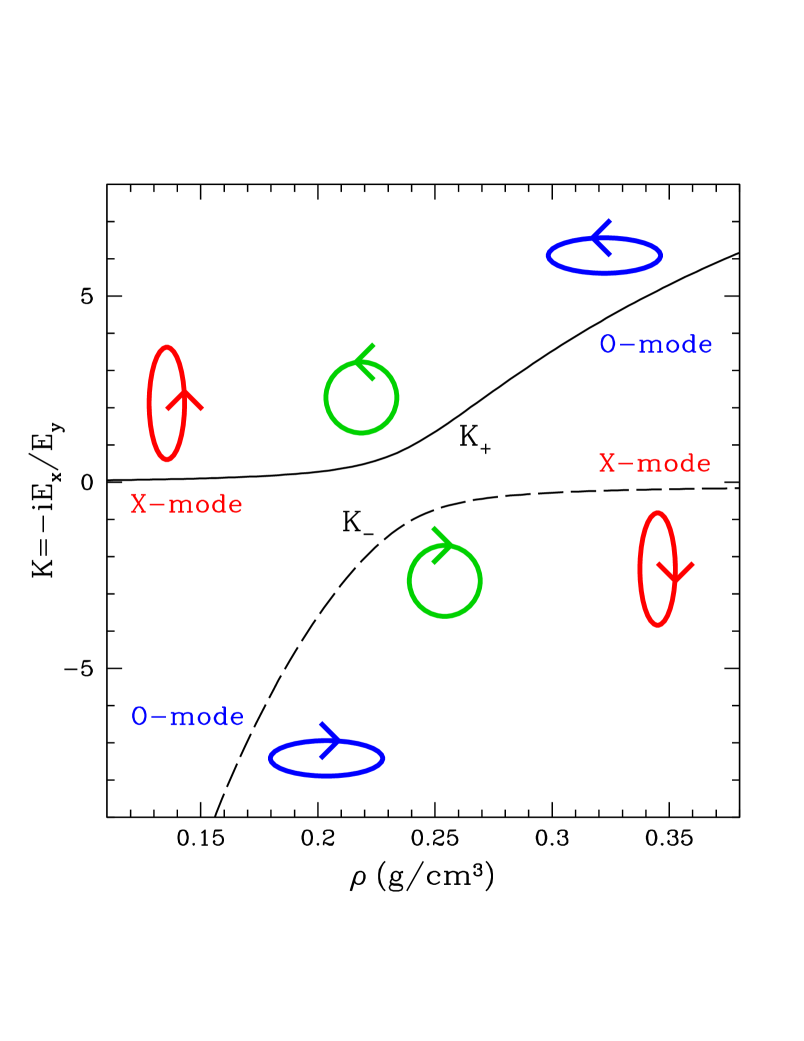
Figure 2: The polarization ellipticity of the photon mode as a function of plasma density near the vacuum resonance. The two curves correspond to the two different modes. In this example, the parameters are $B=10^{13}\,$G, $\epsilon=5\,$keV, $Y_{e}=1$, and $\theta_{kB}=45^{\circ}$. The ellipticity of a mode is specified by the ratio $K=-iE_{x}/E_{y}$, where $E_{x}$ ($E_{y}$) is the photon’s electric field component along (perpendicular to) the ${\bf k}$-${\bf B}$ plane. At densities away from the resonance density $\rho_{V}$, the two modes are almost linearly polarized (with polarization ellipses orthogonal to each other): The O-mode is characterized by $|K|\gg 1$, and the X-mode $|K|\ll 1$. At $\rho=\rho_{V}$, both modes are circularly polarized. In the adiabatic limit, an O-mode (X-mode) photon from the high-density region will convert to the X-mode (O-mode) as it traverses the vacuum resonance density $\rho_{V}$, with its polarization ellipse rotated by $90^{\circ}$.

Including the damping terms in the dielectric tensor gives rise to the phenomenon of mode collapse (see Soffel et al. 1983; Lai & Ho 2003a). This occurs when the two polarization modes become identical, i.e., $K_{+}=K_{-}$ or $n_{+}=n_{-}$. Obviously, at the point of mode collapse, the modal description of radiative transfer breaks down and a rigorous treatment of radiative transfer requires solving the transport equations for the four photon intensity matrix, or Stokes parameters (see Lai & Ho 2003a).

4.4 Wave Propagation in Inhomogeneous Medium

Because of the strong gravity, a neutron star atmosphere has a rather large density gradient, with density scale height of order a few cm’s for $T=10^{6}$ K. When a photon propagates in such an inhomogeneous medium, its polarization state will evolve adiabatically (i.e. following the $K_{+}$ or $K_{-}$ curve in Fig. 2) if the density variation is sufficiently gentle and the modes are sufficiently distinct (i.e., $n_{1}-n_{2}$ is sufficiently large). Away from the vacuum resonance, the adiabatic condition is easily satisfied. At the vacuum resonance, adiabaticity requires (Lai & Ho 2002)

$$\epsilon\mathrel{\raise 1.29167pt\hbox{$>$}\mkern-14.0mu\lower 2.58334pt\hbox{$\sim$}}\epsilon_{\rm ad}(B,\theta_{B},H_{\rho})=1.49\,\bigl{(}f\,\tan\theta_{B}|1-u_{i}|\bigr{)}^{2/3}\left({5\,{\rm cm}\over H_{\rho}}\right)^{1/3}~{}{\rm keV},$$ (63)

where $H_{\rho}=|dz/d\ln\rho|$ is the density scale height (evaluated at $\rho=\rho_{V}$) along the ray. For an ionized Hydrogen atmosphere, $H_{\rho}\simeq 2kT/(m_{p}g\cos\theta)=1.65\,T_{6}/(g_{14}\cos\theta)$ cm, where $T=10^{6}\,T_{6}$ K is the temperature, $g=10^{14}g_{14}$ cm s^-2 is the gravitational acceleration, and $\theta$ is the angle between the ray and the surface normal. In general, the probability for a nonadiabatic “jump” is

$$P_{\rm jump}=\exp\left[-(\pi/2)(\epsilon/\epsilon_{\rm ad})^{3}\right].$$ (64)

Thus for $\epsilon\mathrel{\raise 1.29167pt\hbox{$>$}\mkern-14.0mu\lower 2.58334pt\hbox{$\sim$}}1.3\epsilon_{\rm ad}$, the polarization evolution is highly adiabatic (with $P_{\rm jump}\mathrel{\raise 1.29167pt\hbox{$<$}\mkern-14.0mu\lower 2.58334pt\hbox{$\sim$}}0.03$) even at the vacuum resonance. In this case, an X-mode (O-mode) photon will be converted into a O-mode (X-mode) as it traverses the vacuum resonance. This resonant mode conversion is analogous to the MSW effect of neutrino oscillation (e.g., Haxton 1995). One could also say that in the adiabatic limit, the photon will remain in the same plus or minus branch, but the character of the mode is changed across the vacuum resonance. Indeed, in the literature on radio wave propagation in plasmas (e.g., Budden 1961; Zheleznyakov et al. 1983), the nonadiabatic case, in which the photon state jumps across the continuous curves, is referred to as “linear mode coupling”. It is important to note that the “mode conversion” effect discussed here is not a matter of semantics. The key point is that in the adiabatic limit, the photon polarization ellipse changes its orientation across the vacuum resonance, and therefore the photon opacity changes significantly (see Lai & Ho 2003a).

The concept of adiabatic evolution of photon polarization is also important when we consider wave/photon propagation in neutron star magnetospheres. For example, the normal modes of X-ray photons in the magnetosphere are determined by vacuum polarization (since $\rho\ll\rho_{V}$). As a photon (of a given mode) propagates from the polar cap through the magnetosphere, its polarization state evolves adiabatically following the varying magnetic field it experiences, up to the “polarization-limiting radius” $r_{\rm pl}$, beyond which the polarization state is frozen. This polarization-limiting radius is located where the adiabatic condition breaks down (see Heyl et al. 2003; Lai & Ho 2003b). Another example concerns the radio wave propagation in the magnetosphere, whose dielectric property is dominated by highly relativistic pair plasmas. Such a propagation effect may be responsible for some of the observed polarization changes in radio emission of pulsars (e.g., Cheng & Ruderman 1979; Barnard 1986; Melrose & Luo 2004).

4.5 Warm Plasma and Relativistic Plasma

While the dielectric tensor for cold plasma was derived classically, the quantum calculation, incorporating the quantized nature of electron motion transverse to the magnetic field, yields the same result when the photon wavenumber $k\rightarrow 0$ (e.g., Canuto & Ventura 1972; Pavlov et al. 1980). More precisely, since the size of the Landau wavefunction is of order $\hat{\rho}=(\hbar c/eB)^{1/2}$ [see Eq. (9)], this requires $k_{\perp}\hat{\rho}\ll 1$ (where $k_{\perp}$ is the wave number perpendicular to ${\bf B}$, or the photon energy must satisfy $\epsilon\sin\theta_{B}\ll\sqrt{m_{e}c^{2}E_{ce}}$.

The cold plasma approximation is valid when the thermal velocity of the electron, $V_{T}=(2k_{B}T/m_{e})^{1/2}$, is much less than the phase velocity of the wave ($\omega/k\simeq c$), and $\omega$ is not too close to the cyclotron frequency, i.e., for $|\omega-\omega_{ce}|\gg(\omega/c)V_{T}$ (we neglect the ion component here). The cold plasma approximation also neglects electron recoil. Taking into account the electron motion, the cyclotron resonance denominator $\omega-\omega_{ce}$ in the cold plasma dielectric should be replaced by $\omega-k_{\parallel}V_{\parallel}-\omega_{ce}$ (where $k_{\parallel}$ and $V_{\parallel}$ are the wavenumber and electron velocity parallel to the magnetic field), and the electron recoil can also be included by $\omega\rightarrow\omega\pm\hbar k_{\parallel}^{2}/(2m_{e})$. Then the dielectric tensor should be averaged over the electron velocity distribution function. In the very strong magnetic field limit where electrons occupy only the lowest Landau level ($k_{B}T\ll E_{ce}$), the cold plasma expressions (41) are replaced by (Kirk 1980)

$$\varepsilon=1-v_{e}\left\{1-{\omega_{ce}\over 2V_{T}k_{\parallel}}\Bigl{[}W(y_{-})-W(y_{+})\Bigr{]}\right\},$$ (65)

$$g=-v_{e}{\omega_{ce}\over 2V_{T}k_{\parallel}}\Bigl{[}W(y_{-})+W(y_{+})\Bigr{]},$$ (66)

$$\eta=1-v_{e},$$ (67)

where

$$y_{\pm}={\omega\pm\omega_{ce}\over V_{T}k_{\parallel}}\pm{\hbar k_{\parallel}\over 2m_{e}V_{T}},$$ (68)

[the $\hbar k_{\perp}/(2m_{e}V_{T})$ term arises from electron recoil], and $W(z)$ is the plasma dispersion function

$$W(z)={1\over\sqrt{\pi}}\int_{-\infty}^{\infty}\!{e^{-x^{2}}\,dx\over x-z},$$ (69)

which should be evaluated for $\omega_{ce}\rightarrow\omega_{ce}/(1+i\gamma_{re})$ with $\gamma_{re}>0$ [see Eq. (35)]. Expressions (66)-(67) are valid in the nonrelativistic limit, $\hbar\omega\ll m_{e}c^{2}$ and $k_{B}T\ll m_{e}c^{2}$. One can check that for $|\omega-\omega_{ce}-\hbar k_{\parallel}^{2}/(2m_{e})|\gg|V_{T}k_{\parallel}|$, the cold plasma limit is recovered. The net effect of finite temperature is that the cyclotron resonance is softened from the sharp peak of the cold plasma theory to a broadened one with width $\Delta\omega\sim k_{\parallel}V_{T}$. Also, the electron recoil shifts the resonance by $\Delta\epsilon\simeq(E_{ce}\cos\theta_{B})^{2}/(2m_{e}c^{2})$, which becomes appreciable as $B$ approaches $B_{Q}$. Thus a quantitative description of the cyclotron resonance for $B\mathrel{\raise 1.29167pt\hbox{$>$}\mkern-14.0mu\lower 2.58334pt\hbox{$\sim$}}B_{Q}$ requires relativistic theory (see §5).

Similar qualitative behavior appears in the relativistic theory (e.g., Svetozarova & Tsytovich (1962); Melrose 1974; Pavlov et al. 1980; Nagel 1981; Meszaros & Nagel 1985; see Meszaros 1992 for a review). The polarization tensor is directly proportional to the forward-scattering amplitude of a photon in the plasma. Quantum states and momentum distribution of electrons can be summed or averaged. The advantage of such an approach is that the photon polarization modes are calculated in a self-consistent manner as the differential scattering cross section, which depends on photon modes (see §5).

The magnetosphere of a radio pulsar is believed to be filled with ultra-relativistic electron-positron pairs (see §9). In the polar-cap region, outwardly streaming pair plasmas are produced in an electromagnetic cascade (Sturrock 1971), with bulk Lorentz factor $\gamma\mathrel{\raise 1.29167pt\hbox{$>$}\mkern-14.0mu\lower 2.58334pt\hbox{$\sim$}}10^{2}$ (e.g., Daugherty & Harding 1982; Zhang & Harding 2000; Hibschman & Arons 2001). While the polarization state of high-energy emission is determined by the vacuum polarization effect, radio emission generated in the inner magnetosphere can be affected when propagating through such a plasma (e.g., Cheng & Ruderman 1979; Barnard 1986). For example, the observed characteristics of circular polarization (Radhakrishnan & Rankin 1990; Han et al. 1998) are thought to develop as a propagation effect (e.g., Petrova & Lyubarskii 2000; Melrose & Luo 2004; Petrova 2006). The most important region is associated with the cyclotron resonance, where $\gamma\omega(1-\beta\cos\theta_{B})=\omega_{ce}$. Dispersion in a pulsar plasma has been studied extensively, under various assumptions about the relative electron-positron densities and their momentum distribution, which are uncertain (e.g., Arons & Barnard 1986; Lyutikov 1998; Melrose et al. 1999; Asseo & Riazuelo 2000). A simple model is based on applying a Lorentz transformation to the magneto-ionic (cold plasma) theory (Melrose & Stoneham 1977; Melrose & Luo 2004), which ignores the random motions of the particles. Such a model has been used to interpret the circular polarization in pulsar radio emission (Melrose & Luo 2004). The effect of vacuum resonance in the magnetosphere plasma of pulsars and magnetars is studied by Wang & Lai (2006).

5 Radiative Processes for Free Electrons

At low magnetic field strengths, many of the radiative processes we discuss below, including cyclotron absorption and emission and Compton scattering, may be described by classical physics. In neutron star magnetic fields approaching the critical field, a relativistic quantum description is required to accurately compute the rates and the photon spectrum of radiation, even for non-relativistic electrons. For these processes, we will first review the classical descriptions before discussing the quantum description and discuss the regimes in which each is appropriate. Other processes we will discuss, including one-photon pair production and annihilation, photon splitting and bound pair creation, take place only in strong fields since they do not conserve energy and momentum in free space. In a magnetic field, perpendicular momentum of particles is not conserved in transitions between Landau states since the field effectively is able to supply or absorb momentum. The momentum conservation along the field couples directly to the translational invariance of the system (see Section 2) parallel to B. The conservation equations for energy and parallel momentum for transitions of electrons or positrons between initial state $(n,s,p)$ and final state $(n^{\prime},s^{\prime},p^{\prime})$, where $s=(\sigma_{z}+1)/2$ is the electron spin state, $p=cp_{z}$ and $n$ labels the Landau level [see Eq. (15)], read

$$E_{n}-E_{n^{\prime}}=\pm\epsilon$$ (70)

$$p^{\prime}=p\mp\epsilon\cos\theta$$ (71)

resulting in emission (upper sign) or absorption (lower sign) of photons at angle $\theta$ to the magnetic field with energy $\epsilon$. [In this Section, in contrast to previous Sections, we will express all photon and particle energies in units of $m_{e}c^{2}$.] The photon energy, as determined from the above kinematic equations, is

$$\epsilon=\pm\,\,{(E_{n}-p\cos\theta)-[(E_{n}-p\cos\theta)^{2}-2B^{\prime}(n-n^{\prime})\sin^{2}\theta]^{1/2}\over\sin^{2}\theta},$$ (72)

where in this section, we use $B^{\prime}\equiv B/B_{Q}$ as the dimensionless magnetic field parameter (equivalent to the $\beta$ parameter in section 4). Unless the photon is emitted or absorbed with angle $\theta=90^{0}$, the electron will experience a recoil along the field direction, given by Eqn (71), which is needed to determine its final energy. The electron wavefunctions that have been adopted in the literature for studying the processes presented in the following subsections were discussed in §2.

5.1 Cyclotron Absorption

Cyclotron absorption, the inverse of cyclotron emission (see §5.2), is a first-order process in which a photon excites a particle to a higher Landau state. The classical, non-relativistic cross section for absorption of a photon by an electron at rest in the ground state (n=0) (or in the rest frame of a moving electron) was derived by Blandford & Scharlemann (1976)

$$\sigma^{N}_{\rm abs}(\parallel,\perp)={2\alpha\pi^{2}\lambda\hbox to0.0pt{\hss--}^{2}}\,\delta(\epsilon-NB^{\prime})\left({N^{2}\over 2}B^{\prime}\sin^{2}\theta\right)^{N-1}\,{(\cos^{2}\theta,1)\over(N-1)!},$$ (73)

where $N$ is the harmonic number, $\alpha=1/137$, $\lambda\hbox to0.0pt{\hss--}=\hbar/(m_{e}c)$, $\theta$ is the angle of photon propagation to the magnetic field and the quantity in parentheses refers to the two incident photon linear polarizations $(\parallel,\perp)$ or (O,X) modes, with electric vectors parallel and perpendicular to the plane containing the photon wavevector and the magnetic field. The $\delta$-function restricts the energy of the absorbed photon to be a harmonic, $\epsilon_{N}=NB^{\prime}$, of the cyclotron energy $\epsilon_{B}=E_{ce}/m_{e}c^{2}=B^{\prime}$.

The relativistic QED cyclotron absorption cross section was first derived by Daugherty & Ventura (1978) for electrons initially in the ground state. The required energy for excitation to state $N$ now follows from the relativistic kinematic equations (70) and (71), setting $E_{n}=1$, $n=0,n^{\prime}=N$ and $p=0$,

$$\epsilon_{N}=[(1+2NB^{\prime}\sin^{2}\theta)^{1/2}-1]/\sin^{2}\theta$$ (74)

for a photon propagating at angle $\theta$ to the field. Because the electron experiences a recoil of $p^{\prime}=\epsilon_{N}\cos\theta$ on absorption, the cyclotron harmonics are actually anharmonic in high magnetic fields, so that the energy difference between successive harmonics will decrease. The cyclotron absorption rate, summed over final spin states of the electron, is (Harding & Daugherty 1991)

$$\sigma_{\rm abs}^{N}(\parallel,\perp)={2\alpha\pi^{2}\lambda\hbox to0.0pt{\hss--}^{2}\over E_{N}}\,\delta(\epsilon_{N}-\epsilon)\,{e^{-Z}Z^{N-1}\over(N-1)!}\,\left[(\cos^{2}\theta,1)+{Z\over N}(\sin^{2}\theta,0)\right],$$ (75)

where

$$Z={\epsilon^{2}\sin^{2}\theta\over 2B^{\prime}},$$ (76)

The $\delta$-function requires that the absorbed photon energy have only the value given by equation (74) and effectively makes $\sigma_{\rm abs}^{N}$ only a function of the incident photon angle $\theta$. The above expression reduces to the classical limit of equation (73) when $NB^{\prime}<<1$, where $\epsilon\approx NB^{\prime}$, $Z\approx N^{2}B^{\prime}\sin^{2}\theta/2\ll 1$ and $E_{N}\approx 1$. Therefore, the relativistic formula (75) should be used when $NB^{\prime}\buildrel>\over{\sim}0.1$, that is, when electron recoil becomes significant, which is the case in fields above $\sim 10^{12}$ Gauss.

5.2 Cyclotron and Synchrotron Radiation

Cyclotron radiation is the inverse of the cyclotron absorption process discussed above, and results from downward transitions between Landau levels. The classical cyclotron radiation formula was first presented by Schott (1912) and assumes a continuous circular orbit of the particle in a magnetic field with negligible energy loss. The emission is characterized by the particle velocity $\beta$ and pitch angle, $\psi=\tan^{-1}(\beta_{\perp}/\beta_{\parallel})$, where $\beta_{\parallel}$ and $\beta_{\perp}$ are the velocity parallel and perpendicular to the field direction. If the particle energy is above the cyclotron energy, the radiation is the sum over a number of harmonics of the fundamental cyclotron energy. The radiated power at frequency $\nu$ and angle $\theta$ to the magnetic field is given by (Sokolov & Ternov 1986)

$$W={e^{2}\omega^{2}\over c}\,\sum_{\nu=1}^{\infty}\nu^{2}\,\int_{0}^{\pi}{\sin\theta d\theta\over(1-\beta_{\parallel}\cos\theta)^{3}}{\left\{\left({\cos\theta-\beta_{\parallel}\over\sin\theta}\right)^{2}\,J_{\nu}^{2}(\xi)+\beta_{\perp}^{2}{J^{\prime}_{\nu}}^{2}(\xi)\right\}}$$ (77)

where $\omega=eB/(\gamma m_{e}c)$ is the particle gyrofrequency and

$$\xi={\nu\beta_{\perp}\sin\theta\over 1-\beta_{\parallel}\cos\theta}.$$ (78)

The polarized form of equation (77), in the case where $\beta_{\parallel}=0$, is given in Sokolov and Ternov (1986). The spectrum, given by Bekefi (1966), Canuto and Ventura (1977) and Brainerd and Lamb (1987), display characteristic harmonics at low energy. When the particle energy is relativistic and the emission is dominated by high harmonics, it is called synchrotron radiation. The formula becomes somewhat simpler and the emission power per unit photon energy is (e.g. Jackson 1975)

$$I_{C}(\epsilon)={\sqrt{3}\,\alpha\omega_{B}\sin\psi\over 2\pi}\,\kappa\left({2\epsilon\over 3\gamma\Upsilon\sin\psi}\right),$$ (79)

where $\omega_{B}=\omega_{ce}=eB/(m_{e}c)$ is the cyclotron frequency, $\Upsilon\equiv\gamma B^{\prime}$, $\gamma$ is the electron energy and the $\kappa$ function is

$$\kappa(y)=y\,\int_{y}^{\infty}K_{5/3}(x)\,dx.$$ (80)

The characteristic energy of a synchrotron photon is $\epsilon\sim\gamma^{2}B^{\prime}\sin\psi$.

In high fields approaching the critical field, the classical description should be replaced with a relativistic quantum description to accurately compute the radiative rates and photon spectrum, even for non-relativistic electrons. The classical value of the critical radiation frequency, $\gamma^{2}\epsilon_{B}$, exceeds the electron kinetic energy, $(\gamma-1)$ when

$$B^{\prime}{\gamma^{2}\over(\gamma-1)}>1.$$ (81)

The classical emissivity therefore violates conservation of energy. The classical formula also overestimates the spectral emissivity when

$$\Upsilon\sin\psi\equiv\gamma B^{\prime}\sin\psi>0.1.$$ (82)

There is a consequent reduction of the energy loss rate for large values of $\Upsilon$ (Erber 1966). Finally, taking into account electron recoil gives harmonic energies which are not simple multiples of the cyclotron frequency, as in the non-relativistic case. The polarization and spin dependent transition rates for quantum synchrotron radiation are given by Sokolov & Ternov (1968, see also Harding & Preece 1987) and should be used for transitions between low Landau states in field $B^{\prime}\buildrel>\over{\sim}0.1$. The exact QED spectrum for transition from state $n$ to the ground state $n^{\prime}=0$, averaged over electron spin, is (Latal 1986, Baring et al. 2005)

$${d\Gamma_{n0}\over d\epsilon}= {\alpha c\over\lambda\hbox to0.0pt{\hss--}}{1\over B^{\prime}\varepsilon_{n}^{2}}{n^{n-1}e^{n}\over\Gamma(n+1)}\left({\epsilon\over\epsilon_{-}}-1\right)^{n-1}$$ (83)

$${(\varepsilon_{n}-\epsilon)nB^{\prime}-\epsilon\over\sqrt{(\varepsilon_{n}-1-\epsilon)(\varepsilon_{n}+1-\epsilon)}}\exp\left({-n{\epsilon\over\epsilon_{-}}}\right)$$

where $\varepsilon_{n}\equiv\sqrt{1+2nB^{\prime}}$ and $\epsilon_{-}\equiv nB^{\prime}/\varepsilon_{n}$. The rate is more complicated for transitions between higher Landau states, involving Laguerre polynomials. The cyclotron decay rate from state $n$ is found by integrating over the radiated photon energy in each transition, $\Gamma_{nn^{\prime}}$ and then summing over the final states $n^{\prime}$:

$$\Gamma_{n}=\sum_{n^{\prime}=0}^{n-1}\Gamma_{nn^{\prime}}.$$ (84)

The spin-averaged decay rates for some selected states, as a function of field strength, are shown in Figure 3 and compared to the classical (non-relativistic) values (Herold et al. 1982). One can see that the QED decay rate departs from the classical rate for $B^{\prime}n\buildrel>\over{\sim}0.1$. The spin-dependent decay rates have been discussed by Daugherty & Ventura (1978) and by Melrose & Zheleznyakov (1981) for the non-relativistic case, and by Herold et al. (1982) for the relativistic case. Generally, the probability for spin-flip transitions, those in which the electron changes its spin state, is lower than for non spin-flip transitions. The ratio of the spin-flip decay rate to the non-spin-flip decay rate is $\propto B^{\prime-1}$ for the $n=1\rightarrow 0$ transition.

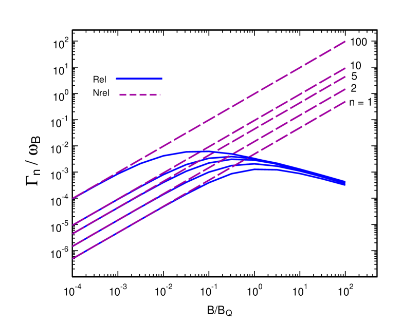
Figure 3: Spin-averaged cyclotron decay rates (solid lines), in units of the cyclotron frequency $\omega_{B}$, from Landau state $n$ as a function of magnetic field strength $B$ in units of the critical field $B_{Q}$. Also plotted are the corresponding non-relativistic decay rates (dashed lines).

An asymptotic form of the spectrum, averaged over spin and polarization, valid for relativistic elections, transitions between high Landau states ($n,n^{\prime}\gg 1$) and zero longitudinal momentum ($\psi=90^{\circ}$), is (Sokolov & Ternov 1968)

$$I_{Q}(\epsilon)={\sqrt{3}\alpha\omega_{B}\over 2\pi}\,(1-{\epsilon\over\gamma})\,\left[\kappa(y)+y^{3}({3\over 2}\Upsilon)^{2}(1-{\epsilon\over\gamma})K_{2/3}(y)\right]$$ (85)

where

$$y={2\epsilon\over 3\gamma\Upsilon[1-(\epsilon/\gamma)]}$$ (86)

One can see that the above expression incorporates a kinematic cutoff in the spectrum at $\epsilon=\gamma$ that avoids energy violation. When $\epsilon\ll\gamma$ and $B^{\prime}\ll 1$, formula (85) reduces to the classical formula (79).

There are several notable features of cyclotron/synchrotron radiation in high magnetic fields. Classically and at low field strengths, rates are highest for single harmonic number transitions and decrease monotonically with increasing harmonic number, with transitions from high Landau states to the ground state being very improbable. But for field strengths $B^{\prime}\buildrel>\over{\sim}0.2$, transitions from high to low states become more probable and transitions to the ground state can actually dominate over even single harmonic number transitions (White 1974, Harding & Preece 1987). The result is that electrons in very high magnetic fields radiate energy not in small steps but often in one large transition, emitting a photon equal to its kinetic energy. The spectrum displays an enhancement just before the kinematic cutoff, as shown in Figure 4.

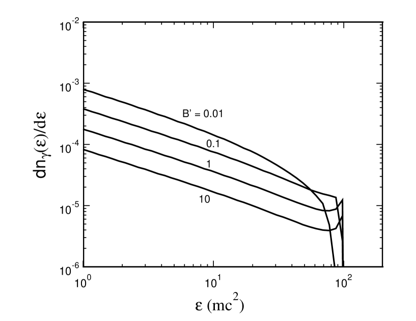
Figure 4: Quantum synchrotron spectra for a particle with Lorentz factor $\gamma=100$, initial pitch angle, $\sin\psi=1$ and different field strengths $B^{\prime}$ in units of the critical field, computed from the asymptotic formula in Eqn (85).

The energy loss rate of an electron emitting synchrotron radiation, resulting from integration of the spectrum of Eqn (85) over photon energy, is shown in Figure 5 as a function of the parameter $\Upsilon$. For low values of $\Upsilon\ll 0.1$, the synchrotron loss rate follows the well-known classical dependence $\dot{\gamma}\propto\Upsilon^{2}$, but begins to depart from the classical dependence for values of $\Upsilon\buildrel>\over{\sim}0.1$. At large values of $\Upsilon\gg 1$, the loss rate follows a milder dependence $\dot{\gamma}\propto\Upsilon^{2/3}$. This softening of the loss rate occurs because the total rate of emission declines at high $\Upsilon$ (Baring 1988).

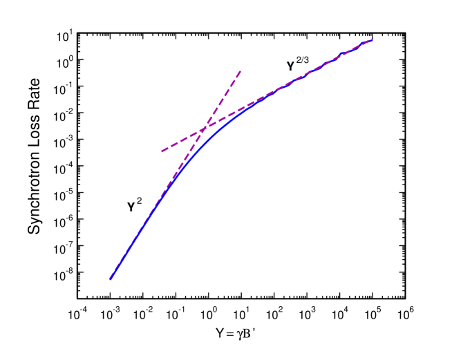
Figure 5: Synchrotron energy loss rate as a function of $\Upsilon=\gamma B^{\prime}$ for an electron having pitch angle $\sin\psi=1$.

5.3 Compton Scattering

In neutron star magnetic fields, the cyclotron decay rate is high enough so that nearly all particles occupy the ground state. The cyclotron de-excitation rate $r_{cyc}\sim 3\times 10^{15}B_{12}^{2}\,\rm s^{-1}$, is much larger the collision rate, $r_{coll}\sim 5\times 10^{8}(n_{e}/10^{21}\,{\rm cm^{-3}})\,B_{12}^{-3/2}\,\rm s^{-1}$ (Bonazzola et al. 1979). Radiative (rather than collisional) processes thus control the Landau state populations. Radiative transitions thus dominate over collisions in astrophysical sources having strong magnetic fields. An electron that absorbs a cyclotron photon will almost always de-excite by emitting another photon, rather than collisionally de-exciting, so that the end result of the process is a scattering of the photon rather than a true absorption. This means that in strong fields resonant scattering dominates over absorption. Cyclotron absorption is most accurately treated as a second-order process, as resonances in the Compton scattering cross section, where the excited state of the particle is a virtual state for which energy and momentum are not strictly conserved. The cyclotron lines are thus broadened by the intrinsic width which is equal to the inverse of the decay rate from that state (Harding & Daugherty 1991, Graziani 1993), although Doppler broadening usually dominates at most angles. The addition of the decay rate to the resonant denominator also renders the cross section finite at resonance. The cross section for Compton scattering in a magnetic field was first studied in the non-relativistic limit by Canuto, Lodenquai & Ruderman (1971) and the full QED cross section has been computed by Herold (1979), Daugherty & Harding (1986) and Bussard, Meszaros & Alexander (1986). Since the non-relativistic treatment is limited to dipole radiation, only scattering at the cyclotron fundamental is allowed. In the relativistic (QED) treatment scattering at higher harmonics is allowed, including Raman scattering, in which the state of the particle after scattering is higher than the initial state.

In free space, the total electron scattering cross section is just the Thomson cross section, $\sigma_{T}=6.6\times 10^{-24}\,\rm cm^{2}$, for photon energies which are non-relativistic in the electron rest frame, or when $\epsilon\gamma\ll m_{e}$. At higher energies, relativistic effects are important both in the kinematics and in the cross section (e.g. Rybicki and Lightman 1979). The photon energy change in the electron rest frame, due to electron recoil, can no longer be ignored and the Klein-Nishina cross section (e.g. Jauch & Rohrlich 1980) is appropriate in the relativistic (QED) regime.

The classical, non-relativistic (Thomson) limit of the magnetized scattering cross section (Canuto et al. 1971, Ventura 1979) has a strong dependence on photon frequency, angle to the magnetic field and polarization. The non-relativistic total scattering cross section in the electron rest frame for linearly polarized photons takes the form (Blandford and Scharlemann 1976):

$$\sigma_{\parallel} = \sigma_{T}\left\{\sin^{2}\theta+{1\over 2}\cos^{2}\theta\left[{\epsilon^{2}\over(\epsilon+\epsilon_{B})^{2}}+{\epsilon^{2}\over(\epsilon-\epsilon_{B})^{2}}\right]\right\}$$

$$\sigma_{\perp} = {\sigma_{T}\over 2}\left\{{\epsilon^{2}\over(\epsilon+\epsilon_{B})^{2}}+{\epsilon^{2}\over(\epsilon-\epsilon_{B})^{2}}\right\}.$$ (87)

for polarization states $(\parallel,\perp)$ where to the photon electric vector parallel or perpendicular to the plane formed by the photon wavevector and the field. Here $\theta$ and $\epsilon$ are the angle and energy of the incident photon with respect to the field in the electron rest frame, and $\epsilon_{B}=\hbar eB/(m_{e}c)$ is the cyclotron energy.

The main effects of the magnetic field on electron scattering is the appearance of the cyclotron resonance and a strong dependence of the cross section on photon energy and incident angle. For photon energies well above the resonance, $\epsilon\gg\epsilon_{B}$, $\sigma=\sigma_{T}$ for both polarizations. For photon energy below the resonance, $\epsilon\ll\epsilon_{B}$, $\sigma_{\parallel}\simeq\sigma_{T}[\sin^{2}\theta+\cos^{2}\theta(\epsilon/\epsilon_{B})^{2}]$ and $\sigma_{\perp}\simeq\sigma_{T}(\epsilon/\epsilon_{B})^{2}$. A magnetized plasma becomes quite optically thin for propagation parallel to the magnetic field for photon frequencies below the cyclotron frequency.

As in the case of cyclotron absorption, the non-relativistic cross section for scattering is not accurate for $B^{\prime}\buildrel>\over{\sim}0.1$ and furthermore describes scattering only in the fundamental and so cannot be used to treat scattering in higher harmonics. As we will discuss in more detail in §11, cyclotron line modeling at low field strengths is still possible using the absorption cross section for harmonics above the fundamental, where the scattering is treated as cyclotron absorption followed by cyclotron emission of the photon. Even at high field strengths, use of the relativistic absorption cross section can give a reasonable approximation to the scattering cross section for low harmonics. But this treatment neglects the contribution from non-resonant scattering which is important for photon energies away from resonance.

The relativistic magnetic scattering cross section is quite complicated even for the simplest case of ground state-to-ground state scattering (Herold 1979), and is even more unwieldy for the case of scattering to arbitrary Landau states (Daugherty & Harding (1986) and Bussard, Meszaros & Alexander 1986). However, a number of interesting features appear in the relativistic scattering cross section (Daugherty & Harding 1986). One is the possibility of ground state-to-ground state scattering through higher intermediate Landau states (i.e. $0\rightarrow n\rightarrow 0$, producing resonant contributions to the cross section at higher harmonics. Another possibility is a $0\rightarrow 0\rightarrow n$ scattering where a photon of energy $\epsilon\simeq nB^{\prime}$ is almost completely ‘absorbed’ producing a scattered photon having very low energy. The inverse process in which an electron in an excited state scatters to the ground state, can convert an X-ray photon to a $\gamma$-ray photon (Brainerd 1989). Another possibility that arises solely in QED is two-photon emission, where an electron makes a transition between two Landau states with the emission of two photons (Alexander & Meszaros 1991a, Semionova & Leahy 1999, Melrose & Kirk 1986) Gonthier et al. (2000) have derived a simplified analytic approximation to the relativistic Compton scattering cross section for the case where the incident photon is parallel to the field, in which case there is a resonance only at the fundamental and scattering to higher Landau states can effectively be neglected. Such a situation would apply to scattering by a relativistic electron moving along the magnetic field, where photons would primarily appear predominatly in a Lorentz cone ($1/\gamma$) centered on the field direction in the electron rest frame. The approximate expression for the total relativistic, polarization-dependent scattering cross section for the case $\theta=0^{\circ}$ is

$$\sigma_{||\to||} = \sigma_{\perp\to||}={{3\sigma_{T}}\over{16}}\left\{{g(\epsilon)-h(\epsilon)}\right\}\left[{{1\over{(\epsilon-B^{\prime})^{2}}}+{1\over{(\epsilon+B^{\prime})^{2}}}}\right],$$

$$\sigma_{||\to\perp} = \sigma_{\perp\to\perp}={{3\sigma_{T}}\over{16}}\left\{{f(\epsilon)-2\epsilon h(\epsilon)}\right\}\left[{{1\over{(\epsilon-B^{\prime})^{2}}}+{1\over{(\epsilon+B^{\prime})^{2}}}}\right]\$$ (88)

where

$$g(\epsilon) = {{\epsilon^{2}(3+2\epsilon)+2\epsilon}\over{\sqrt{\epsilon(2+\epsilon)}}}\ln\left({1+\epsilon-\sqrt{\epsilon(2+\epsilon)}}\right)+{\epsilon\over 2}\ln(1+4\epsilon)$$

$$+\epsilon(1+2\epsilon)\ln(1+2\epsilon)+2\epsilon,$$

$$f(\epsilon) = -\epsilon^{2}\ln(1+4\epsilon)+\epsilon(1+2\epsilon)\ln(1+2\epsilon),\ {\rm and}$$ (89)

$$h(\epsilon) = \left\{\begin{array}[]{ll}{{\epsilon^{2}}\over{\sqrt{\epsilon(2-\epsilon)}}}\tan^{-1}\left({{{\sqrt{\epsilon(2-\epsilon)}}\over{1+\epsilon}}}\right),&\mbox{for $\epsilon<2$, and}\\ {{\epsilon^{2}}\over{2\sqrt{\epsilon(\epsilon-2)}}}\ln\left({{{\left({1+\epsilon+\sqrt{\epsilon(\epsilon-2)}}\right)^{2}}\over{1+4\epsilon}}}\right),&\mbox{for $\epsilon>2$.}\end{array}\right.$$ (92)

This expression reduces to the nonrelativistic limit for small $\epsilon$. Figure 6 shows this approximation compares to the exact QED cross section for the same case of incident photon angle $\sin\theta=0$. For incident photon energies above the cyclotron energy, the electron can be excited to higher Landau states and this contribution (for states up to $n^{\prime}=500$) is included in the exact cross section. Even though the approximation assumed only $n^{\prime}=0$, it does surprisingly well. For photon energies well above $\epsilon_{B}$, the cross section tends toward the field-free relativistic (Klein-Nishina) cross section. The suppression of the relativistic magnetic cross section is due primarily to Klein-Nishina effects, i.e. electron recoil. The approximation for the differential scattering cross section for this case is given in Gonthier et al. (2000).

1

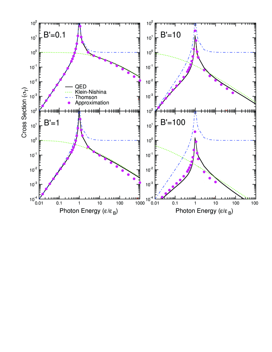
Figure 6: Total polarization-averaged Compton scattering cross section for an electron at rest in the ground state, in units of the Thompson cross section, as a function of incident photon energy in units of cyclotron energy, for the case of incident photon angle $\sin\theta=0$. Solid line: relativistic QED cross section (e.g. Bussard et al. 1986, Daugherty & Harding 1986) summed over final electron Landau states up to 500, dot- dashed line: magnetic Thompson cross section, Eqn. (5.3), dotted line: Klein-Nishina (non-magnetic) cross section, dots: approximate QED cross section in Eqn (5.3). Adapted from Gonthier et al. (2000).

5.4 Pair Production and Annihilation

In a strong magnetic field, single photons as well as two or more photons may convert into electron-positron pairs. One-photon pair production cannot conserve both energy and momentum in field-free space, but a magnetic field can absorb the extra momentum of a photon with the energy required to created a pair.

5.4.1 One-photon pair creation and annihilation

A photon with energy $\epsilon$, traveling at angle $\theta$ to the magnetic field, can produce an electron with parallel momentum $p$ and a positron with parallel momentum $q$ only in the discrete Landau states that are kinematically allowed by the energy and momentum conservation equations,

$$E_{n}+E_{n^{\prime}}=\epsilon$$ (93)

$$p+q=\epsilon\cos\theta$$ (94)

where $E_{n}=(1+p^{2}+2nB^{\prime})^{1/2}$ and $E_{n^{\prime}}=(1+q^{2}+2n^{\prime}B^{\prime})^{1/2}$ are the energies of the electron and positron. The threshold, $\epsilon=2/\sin\theta$, is the photon energy needed to produce a pair with momenta $p=q=\epsilon\cos\theta/2$ in the ground state ($n=n^{\prime}=0$). In the case of high photon energies and low magnetic fields, $\epsilon^{2}\sin^{2}\theta/B^{\prime}\gg 1$, where the pair is produced far above threshold in high Landau states, the polarization-averaged pair production attenuation coefficient can be expressed in the asymptotic form (Klepikov 1954, Erber 1966)

$$R_{1\gamma}^{\rm pp}(\chi)={\alpha\over 2\lambda\hbox to0.0pt{\hss--}}B^{\prime}\sin\theta\,\,\,T(\chi),$$ (95)

$$T(\chi)\approx 4.74\chi^{-1/3}{\rm Ai}^{2}(\chi^{-2/3})=\left\{\begin{array}[]{lr}0.377\exp\mbox{\Large$(-{4\over 3\chi})$}&\chi\ll 1\\ \\ 0.6\chi^{-1/3}&\chi\gg 1\end{array}\right.$$ (96)

where $\chi\equiv\epsilon B^{\prime}\sin\theta/2$, Ai is the Airy function and $\lambda\hbox to0.0pt{\hss--}$ is the electron Compton wavelength. The probability of one-photon pair production thus rises exponentially with increasing photon energy and transverse field strength. A rule-of-thumb is that magnetic pair production will be important for this regime when the argument of the exponential in Eqn (95) approaches unity, or when $\chi\geq 0.1$. When the magnetic field $B^{\prime}\buildrel>\over{\sim}0.1$, this condition will be satisfied below the threshold, so that in such high fields pair production will occur near threshold. The pair will then be produced in low Landau states and the attenuation coefficient will exhibit resonances at the threshold for each pair state (Toll 1952, Daugherty & Harding 1983). Eqn (95) will not be valid in this case, but may be corrected for near-threshold effects by making the substitution, $\chi\rightarrow\chi/F$, where $F=1+0.42(\omega\sin\theta)^{-2.7}$ in Eqn (95) (Daugherty & Harding 1983), or by using the approximate expression (Baring 1988, see corrections in Baring 1991)

$$R_{1\gamma}^{\rm pp}(\epsilon,\theta)\simeq{\alpha\over\lambda\hbox to0.0pt{\hss--}}\,{B^{\prime}\sin\theta\over\epsilon_{\perp}^{2}}\,{3\epsilon_{\perp}^{2}-4\over 2(\epsilon_{\perp}+2)^{2}}\,\left[\log{(1/\zeta)}\right]^{-1/2}\,\left[{4\epsilon_{\perp}\over\epsilon_{\perp}^{2}-4}+\log{\zeta}\right]^{-1/2}$$

$$~{}~{}~{}~{}~{}~{}~{}~{}~{}~{}~{}~{}~{}\exp\left\{{-{\epsilon_{\perp}\over B^{\prime}}-{\epsilon_{\perp}^{2}-4\over 4B^{\prime}}\,\log{\zeta}}\right\},~{}~{}~{}~{}~{}~{}~{}~{}~{}~{}~{}~{}~{}~{}2<\epsilon_{\perp}\ll 1/B^{\prime}.$$ (97)

where $\epsilon_{\perp}\equiv\epsilon\sin\theta$, $\zeta=(\epsilon_{\perp}-2)/(\epsilon_{\perp}+2)$. Either of the above prescriptions will approximate the decrease in $R_{1\gamma}$ near threshold (see Figure 7). Semionova & Leahy (2001) have derived the one-photon pair production attenuation coefficient for all cases of photon polarization and electron and positron spin states, making use of the proper spin eigenstates defined by Sokolov & Ternov (1986).

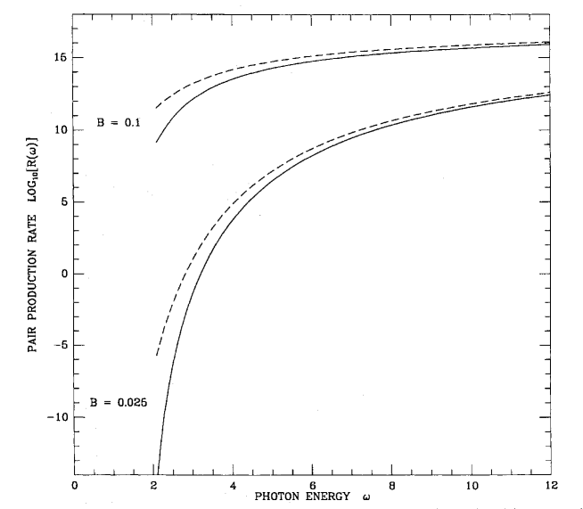
Figure 7: One-photon pair production rate as a function of photon energy (in units of $mc^{2}$), for two different magnetic field strengths (in units of the critical field). The solid lines are the approximation of Eqn (5.4.1) to the exact rate and the dashed lines are the asymptotic formula of Eqn (95). From Baring (1988).

In the case where an electric field is present perpendicular to the magnetic field, the pair production attenuation coefficient can be obtained by a Lorentz transformation perpendicular to the magnetic field (Daugherty & Lerche 1975). When an electric field of strength $E$ parallel to the magnetic field is present, Daugherty & Lerche (1976) determined that the pair attenuation coefficient is increased by an additional amount of order $E^{2}/B^{2}$, which is usually small in neutron star magnetospheres since $E\ll B$ is always true for rotationally induced electric fields.

The inverse process to one-photon pair creation is one-photon pair annihilation, in which an electron-positron pair annihilates into a single photon and is likewise only permitted in a strong field. The kinematic equations are the same as those for one-photon pair creation, Eqns (93) and (94), with the electron and positron initially occupying Landau states $n$ and $n^{\prime}$ with momenta $p$ and $q$. The annihilation rate for pairs in the ground state, $n=n^{\prime}=0$ has been calculated by Wunner (1979) and Daugherty & Bussard (1980) and the expression in the center-of-momentum frame (where $p=-q$) is particularly simple:

$$R_{1\gamma}^{\rm ann}(E_{p})=n_{o}^{+}n_{o}^{-}\,{\alpha\lambda^{2}c\over B^{\prime}}{1\over E_{p}^{2}}\exp\left({-2E_{p}^{2}\over B^{\prime}}\right),$$ (98)

where $\lambda\equiv 2\pi\lambda\hbox to0.0pt{\hss--}$ is the electron Compton wavelength, $E_{p}=(p^{2}+1)^{1/2}$ and $n_{o}^{+}$ and $n_{o}^{-}$ are the number densities of positrons and electrons. The annihilation rate in an arbitrary frame can be obtained by a Lorentz transformation along the magnetic field direction. Since the rate in Eqn (98) increases exponentially with increasing field strength, one-photon annihilation overtakes the two-photon annihilation rate for pairs at rest at a field strength around $10^{13}$ Gauss. One-photon annihilation from the ground state results in a line at $2m$, broadened asymmetrically toward higher energies by the parallel momenta of the pairs. Unlike in the case of two-photon annihilation (cf. §5.4.2), Doppler broadening results only in a blueshift here, because the photon must take all of the kinetic energy of the pair in addition to the rest mass. The annihilation photons are emitted in a fan beam transverse to the field, which is broadened if the pairs have nonzero parallel momenta. Pairs annihilating from excited states produce additional lines above 1 MeV which at high energies blend together into a continuum. The one-photon annihilation rate of pairs from excited states can proceed at a rate orders of magnitude faster than from the ground state in fields below $10^{13}$ G (Harding 1986, Wunner et al. 1986). The one-photon rate therefore becomes comparable to the two-photon rate (which does not rise rapidly in excited states) at lower field strengths for pairs in excited states. However, the effectiveness of synchrotron cooling may keep the densities of excited states low enough relative to the ground state to cancel the increase in the annihilation rate. The one-photon annihilation rate for different photon polarizations and particle spin states has been derived by Wunner et al. (1986) and Semionova & Leahy (2000).

5.4.2 Two-photon pair creation and annihilation in a strong magnetic field

Pair creation by two photons is significantly modified by strong magnetic fields from its field-free behavior. In field-free, the two-photon pair production cross section near threshold in terms of the photon energy in the center-of-momentum frame, $\epsilon_{{}_{\rm CM}}=[\epsilon_{1}\epsilon_{2}(1-\cos\theta_{12})/2]^{1/2}$, is (Svensson 1982)

$$\sigma_{2\gamma}\simeq{3\over 8}\,\sigma_{T}\left\{\begin{array}[]{lr}(\epsilon_{{}_{\rm CM}}^{2}-1)^{1/2}&(\epsilon_{{}_{\rm CM}}-1)\ll 1\\ {\left[2\ln(2\epsilon_{{}_{\rm CM}})-1\right]}/\epsilon_{{}_{\rm CM}}^{6},&\epsilon_{{}_{\rm CM}}\gg 1\\ \end{array}\right.$$ (99)

where $\epsilon_{1}$ and $\epsilon_{2}$ refer to the energies of the photons and $\cos\theta_{12}$ is the cosine of the angle between their propagation directions. The full relativistic cross section can be found in Jauch and Rohrlich (1980). In a magnetic field, the kinematic equations for this process impose conservation of energy and parallel momentum only:

$$\epsilon_{1}+\epsilon_{2}=E_{n}+E_{n^{\prime}}$$ (100)

$$\epsilon_{1}\cos\theta_{1}+\epsilon_{2}\cos\theta_{2}=p+q,$$ (101)

where $\theta_{1}$ and $\theta_{2}$ are their angles with respect to the field. The threshold depends on photon polarization direction with respect to the field, with the threshold for producing a pair in the ground state ($n=n^{\prime}=0$), taking the form (Daugherty and Bussard 1980):

$$(\epsilon_{1}\sin\theta_{1}+\epsilon_{2}\sin\theta_{2})^{2}+2\epsilon_{1}\epsilon_{2}[1-\cos(\theta_{1}-\theta_{2})]\geq 4.$$ (102)

The second term is similar to the field-free threshold condition and the first term appears as a result of non conservation of perpendicular momentum. Thus it is possible for photons traveling parallel to each other ($\theta_{1}=\theta_{2}\neq 0^{0}$) to produce a pair, an event not permitted in field-free space.

The two-photon pair production cross section in a strong magnetic field, like the one-photon pair production cross section, has resonances near threshold due to the discreteness of the pair states. The two-photon cross section in a strong magnetic field has been calculated by Kozlenkov and Mitrofanov (1987) for photon energies below one-photon pair production threshold and shows the same sawtooth behavior as the one-photon process. Near threshold, the magnetic field decreases the cross section below its free-space value, due to the decreased phase space available to the pair. Above its threshold, one-photon pair creation will dominate since it is a lower order process than two-photon pair creation. A comparison of the relative importance of the one-photon and two-photon processes (Burns and Harding 1984) shows that the one-photon process will generally dominate in magnetic fields above $\approx 10^{12}$ Gauss.

The free-space cross section for two-photon pair annihilation in the non-relativistic limit is $\sigma_{2\gamma}=(3/8)\sigma_{T}/\beta_{r}$, where $\beta_{r}$ is the relative velocity of the positron and electron. The annihilation rate for unpolarized positrons and electrons with densities $n_{+}$ and $n_{-}$ is then

$$R_{2\gamma}={3\over 8}\sigma_{T}cn_{+}n_{-}.$$ (103)

The two-photon annihilation rate in a strong magnetic field has been calculated for pairs in the ground Landau state (Daugherty and Bussard 1980, Wunner 1979) and is unchanged from the field-free rate below $B^{\prime}\sim 0.1$. At $B^{\prime}\buildrel>\over{\sim}0.2$, the rate decreases sharply due to the smaller phase-space of the virtual pair states, just as the one-photon annihilation rate is increasing exponentially. Two-photon annihilation of non-relativistic pairs results in a line at 511 keV as in free space, but the relaxation of transverse momentum conservation in a magnetic field causes a broadening mostly on the red side of the line at viewing angles other than $90^{\circ}$. At a viewing angle of $90^{\circ}$ to the field direction, the broadening is symmetric for $B^{\prime}\lower 2.0pt\hbox{$\,\buildrel\scriptstyle<\over{\scriptstyle\sim}\,$}0.1$ but becomes asymmetrically broadened on toward the blue side for $B^{\prime}\buildrel>\over{\sim}0.1$, as shown in Figure 8. The magnetic broadening can be approximated as

$$(\Delta\epsilon)^{B}\sim\left\{\begin{array}[]{lr}B^{\prime}/2,&\sin\theta<\sqrt{2B^{\prime}}\\ \sin\theta\sqrt{B^{\prime}/2},&\sin\theta>\sqrt{2B^{\prime}}\\ \end{array}\right.$$ (104)

There is an increasing tendency in very high fields for one of the photons to be produced with almost all of the pair energy, so that two-photon annihilation behaves more like one-photon annihilation. The angular distribution of the photons from annihilation at rest also becomes more anisotropic with increasing field strength, with the peak of emission perpendicular to B , again similar to one-photon annihilation. Similar broadening occurs when the pairs have non-zero momenta parallel to the magnetic field (Kaminker et al. 1987, Baring & Harding 1992).

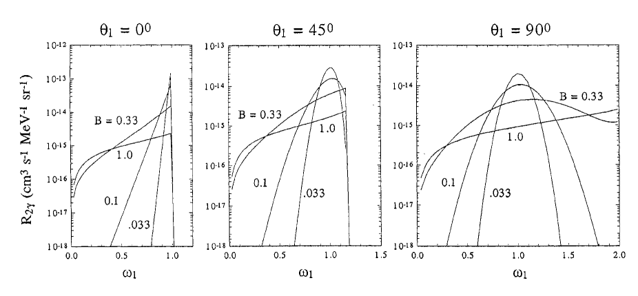
Figure 8: Two-photon annihilation spectra for pairs at rest in a magnetic field in the ground Landau state, for different field strengths (in units of the critical field) and viewing angles to the field, $\theta_{1}$. The kinematic cutoffs occur when $|\cos\theta_{2}|=1$, where $\theta_{2}$ is the angle of the unseen photon. From Baring & Harding (1992).

5.5 Bound Pair Creation

As was first noted by Shabad & Usov (1982), the dispersion curve (as shown in Figure 9) of a photon propagating along a curved magnetic field, with $\epsilon<2/\sin\theta$ initially below the threshold for one-photon pair creation, will cross the lowest bound state of positronium prior to reaching the threshold for creating a free pair in the ground state ($n=n^{\prime}=0$ for $\parallel$ polarization, $n=0,n^{\prime}=1$ or $n=1,n^{\prime}=0$ for $\perp$ polarization). This situation was originally interpreted as a “capture” of the photon by the magnetic field for $B^{\prime}\buildrel>\over{\sim}0.1$, and a complete prevention of free pair creation until the photon could travel to a region of lower field strength. But Herold et al. (1985) pointed out that as the photon approaches the crossing point, it will adiabatically convert into positronium, after evolving through a mixed photon-positronium state (Shabad & Usov 1985, 1986), if the magnetic field is strong enough. The positronium state produced in this way from a single photon is stable to annihilation, since positronium cannot annihilate from the ground state in a magnetic field (Wunner et al. 1981). In this case, creation of a free pair is suppressed unless the positronium is unbound and several possible mechanisms have been discussed. Positronium may be ionized by an electric field parallel to the magnetic field, whose strength is sufficient when combined with the Coulomb field to form a potential barrier low enough for the electron and positron to tunnel through to become a free pair. The probability of ionization by a field of strength $E_{\parallel}$ is (Usov & Melrose 1995)

$$W_{\rm E}={eE_{\parallel}\over 2mc(\Delta\varepsilon_{00})^{1/2}}\,\exp\left[{-4(\Delta\varepsilon_{00})^{3/2}\over 3(eE_{\parallel}/mc^{2})\lambda\hbox to0.0pt{\hss--}}\right]$$ (105)

where $\Delta\varepsilon_{00}$ is the positronium binding energy in the ground state. On the scale of a neutron star radius, R, the critical ionizing field strength, below which the ionization probability is negligible, is

$$E_{\parallel}^{\rm ion}\approx{2\over 3}{mc^{2}(\Delta\varepsilon_{00})^{3/2}\over{e\lambda\hbox to0.0pt{\hss--}}}$$ (106)

and is a slowly varying function of $B^{\prime}$. For $B^{\prime}\sim 0.2$, $eE_{\parallel}^{\rm ion}\sim 10^{10}\,\rm Volts\,cm^{-1}$. Alternatively, the bound pair could be photoionized by a UV radiation field of sufficient intensity (Herold et al. 1985). For example, in a blackbody radiation field of temperature $T_{6}=T/10^{6}$ K the mean-free path for photoionization of positronium moving with Lorentz factor $\Gamma$ in a magnetic field $B^{\prime}\sim 0.1$ is approximately (Bhatia et al. 1992)

$$\ell_{\rm ph}\simeq 5\times 10^{4}\,{\rm cm}\,\left({\Gamma\over 10^{2}}\right)^{3}\,T_{6}^{2}$$ (107)

For $T>10^{5}$ K, the photoionization mean-free path of positronium will be short enough to free a bound pair in a fraction of a neutron star radius.

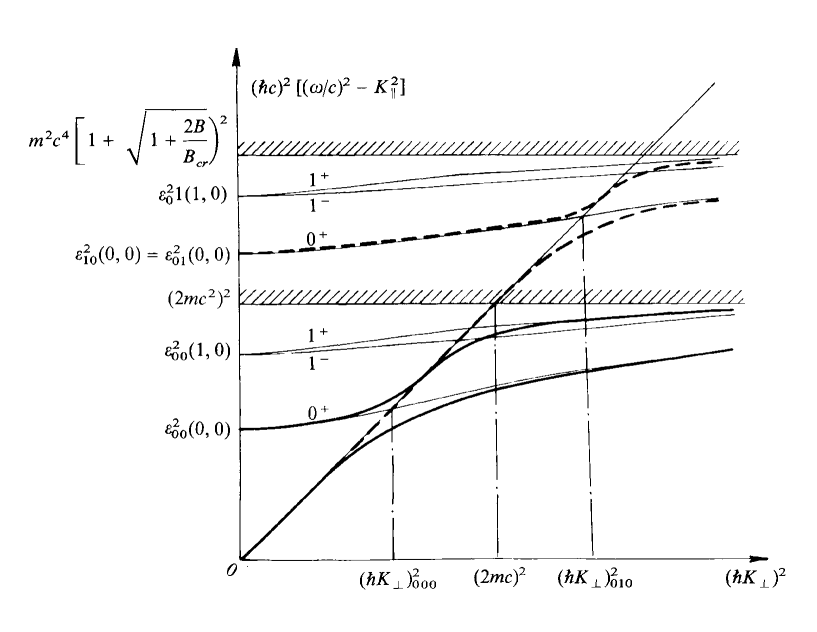
Figure 9: Dispersion curves for photons propagating in a strong magnetic field. The sloped straight line is the unperturbed dispersion curve $(\omega/c)^{2}-K^{2}_{\parallel}=K^{2}_{\perp}$. $\epsilon_{n,n^{\prime}}(n_{c},p_{c})$ are the energies of the positronium states with quantum number $n_{c}$ and parallel momentum $p_{c}$. The thin solid curves, labeled by $n_{c}^{\pm}$, are the positronium dispersion curves for the lowest states having $n=n^{\prime}=0$ and $n+n^{\prime}=1$ for the electron and positron Landau states, where $\pm$ are the parities. The hatched borders are the thresholds for production of a free pair in the two lowest states, which are the same as the positronium continua for each series of states. The thick solid curves are the lowest dispersion curves of the mixed photon-positronium states with $n=n^{\prime}=0$. The thick dashed lines are the lowest dispersion curves for the $n+n^{\prime}=1$ mixed states. From Shabad & Usov (1985).

5.6 Photon Splitting

Photon splitting is a third-order process in which one photon divides into two or more photons in the presence of a strong external field. This process can be most easily understood in the context of the vacuum polarization effect on photon propagation in a strong magnetic field, which is due to the interaction of the photon virtual pairs with the field. To lowest order, photon splitting occurs when one member of a vacuum polarization pair radiates. While it is kinematically allowed in field-free space, it is forbidden by Furry’s theorem (Furry 1937, Jauch & Rohrlich 1980), a QED charge conjugation symmetry stating that the S-matrix vanishes for any closed diagram with an odd number of vertices having only external photon lines. The symmetry is broken by a strong magnetic field. The photon splitting rate in a magnetic field was computed by Bialynicka-Birula & Bialynicki-Birula (1970), and Adler et al. (1970, 1971) in the weakly dispersive limit. In this limit, there are three photon polarization modes permitted by QED (i.e., they do not violate CP conservation): $\perp\rightarrow\parallel\parallel$, $\parallel\rightarrow\perp\parallel$ and $\perp\rightarrow\perp\perp$. A simplified expression (for $B^{\prime}\lower 2.0pt\hbox{$\,\buildrel\scriptstyle<\over{\scriptstyle\sim}\,$}1$) for the polarization-dependent attenuation coefficient for photon splitting was derived by Baring (1991):

$$R^{sp}_{\perp\rightarrow\parallel\parallel}={1\over 2}R^{sp}_{\parallel\rightarrow\perp\parallel}=\left({13\over 24}\right)^{2}R^{sp}_{\perp\rightarrow\perp\perp}={1\over 6}\left({26\over 19}\right)^{2}R_{sp}$$ (108)

and

$$R_{sp}\approx{\alpha^{3}\over 10\pi^{2}\lambda\hbox to0.0pt{\hss--}}\left({19\over 315}\right)^{2}\,B^{\prime 6}\epsilon^{5}\sin^{6}\theta$$ (109)

where $\epsilon$ is the incident photon energy propagating at angle $\theta$ to the magnetic field of strength $B^{\prime}$. Since there is no threshold for photon splitting the expression above is valid for arbitrarily small photon energies. For large values of $B^{\prime}>1$, the $B^{\prime}$ dependence in Eqn (109) saturates (i.e., the factor $B^{\prime 6}\rightarrow 1$ for $B^{\prime}\gg 1$). The full expression for the photon splitting attenuation coefficient is given by Adler (1971) and Stoneham (1979).

Since photon splitting is a third order process, its rate is smaller than that of one-photon pair production above $\epsilon=2/\sin\theta$. However, it can compete with one-photon pair production in neutron star magnetospheres, where photons are below pair creation threshold at their emission points (see §9). As the photon travels in a region of curved field lines, its angle to the field increases and the photon may split before reaching pair creation threshold (Baring 1991, 1995, Harding et al. 1997). Since the photon splitting rate is very sensitive to field strength, its influence grows quickly with increasing field strength with the switch from pair creation to photon splitting being dependent on field geometry. For photons propagating in neutron star dipole magnetic field geometry, photon splitting becomes dominant as an attenuation mechanism for $B^{\prime}\buildrel>\over{\sim}1$ (Baring & Harding 1998).

Adler (1971) examined the kinematic selection rules for photon splitting in the weakly dispersive limit and found that only the $\perp\rightarrow\parallel\parallel$ mode conserved energy and momentum in the magnetized vacuum [another channel, $\perp\rightarrow\parallel\perp$, is also allowed kinematically, but the rate is suppressed by a factor of order $n_{\parallel}-1$ (see Eq. 60) compared to the $\perp\rightarrow\parallel\parallel$ channel, and thus is negligible in the weakly dispersive limit]. Usov (2002), including only the linear positronium contribution to the polarization tensor, has shown that Adler’s kinematic selection rules hold in arbitrarily high magnetic fields. However, the moderate vacuum dispersion present in magnetar fields (see §10) may critically depend on higher order (non-linear) contributions from the polarization tensor (e.g. Melrose and Parle 1983). If Adler’s selection rules are in fact ubiquitous it has profound implications, since it means that the only polarization mode permitted to split produces only photons of the mode that cannot split. Such a situation will prevent pure photon splitting cascades (Baring 1995, Harding & Baring 1996), where the two product photons of an initial splitting split into two more photons, each of which split further, reprocessing the spectrum to lower and lower energies. Such a selection rule also leads to an extremely strong polarizing mechanism, since only one mode is attenuated and produces photon of the other mode. Bulik (1998) has derived the photon splitting rate including the effect of a plasma. He finds that the presence of a plasma changes the kinematic selection rules, allowing addition splitting modes to become important. However, these changes seem to operate only in a small region of phase space in neutron star atmospheres, between $B^{\prime}\sim 0.1-2$, $\theta<30^{\circ}$ and plasma density $\rho>1\,\rm g\,cm^{-3}$.

6 Physics of Neutron Star Interiors and Envelopes

6.1 Overview

Many observable properties of neutron stars, such as the mass-radius relation, the maximum rotation rate and the thermal evolution, depend on the properties of the star’s interior (e.g., Baym & Pethick 1979; Shapiro & Teukolsky 1983; Glendenning 2000; Heiselberg 2002; Lattimer & Parkash 2005). An important goal of neutron star astrophysics is to use various observations of neutron stars to probe the property of matter under extreme conditions, particularly at super-nuclear densities.

A neutron star can be divided into several different regions: the atmosphere/envelope, the crust and the core. The atmosphere/envelope contains a negligible amount of mass, but plays an important role in determining the emergent photon spectrum and flux (see §8). The crust, constituting $1-2\%$ of the stellar mass and extending $\sim 1$ km below the surface, contains atomic nuclei embedded in an electron Fermi sea. Since a neutron star is formed as a collapsed, hot ($k_{B}T\mathrel{\raise 1.29167pt\hbox{$>$}\mkern-14.0mu\lower 2.58334pt\hbox{$\sim$}}10$ MeV) core of a massive star in a supernova explosion, the neutron star matter may be assumed to be fully catalyzed and in the absolute lowest energy state (e.g., Salpeter 1961; Baym, Pethick & Sutherland 1971). The dominant nuclei in the crust vary with density, and ranges from ⁵⁶Fe at $\rho\mathrel{\raise 1.29167pt\hbox{$<$}\mkern-14.0mu\lower 2.58334pt\hbox{$\sim$}}8\times 10^{6}$ g cm^-3 to neutron-rich nuclei with $A\sim 200$ and $Z/A\sim 0.1$ near the core-crust interface at $\rho\sim 10^{14}$ g cm^-3 (see Douchin & Haensel 2001 for recent work on neutron star crust composition). This “standard” picture of neutron star crust, in which one particular kind of nucleus is present at a given density and these nuclei form a near-perfect crystal lattice, has been challenged by Jones (1999), who argued that thermodynamic fluctuations at the time of freezing would ensure the presence of several kinds of nuclei at a given pressure, yielding an impure solid. This would substantially increase the resistivity of the crust, particularly at low temperatures, and thus greatly affect magnetic field evolution and heat conduction in the crust (Jones 2004). At densities above the $4\times 10^{11}$ g cm^-3, neutrons “drip” out of nuclei and permeate the crust (this region is called “inner crust”). At temperatures less than $\sim 0.1$ MeV, these neutrons are expected to form Cooper pairs and turn superfluid, largely decoupling dynamically from the rest of the star. This has been invoked to explain pulsar glitches, quick increases of the observed rotation rate the star, which might be caused by a sudden transfer of angular momentum from the more rapidly rotating neutron superfluid to the crust. Around the highest density region in the crust, the nuclei may assume rod- and plate-like shapes (“nuclear pasta”; Pethick & Ravenhall 1995), before an eventual transition to uniform nuclear matter of the liquid core.

The liquid core (with densities $\mathrel{\raise 1.29167pt\hbox{$>$}\mkern-14.0mu\lower 2.58334pt\hbox{$\sim$}}2\times 10^{14}$ g cm^-3) consists of a mixture of neutrons, protons and electrons, which at progressively higher densities are joined by muons and other exotic particles such as strangeness-bearing hyperons and/or pion or kaon Bose condensates. Chemical equilibrium among these particles is established by weak interactions such as neutron beta decay ($n\rightarrow p+e^{-}+\bar{\nu}$) and electron capture ($e^{-}+p\rightarrow n+\nu$), and the nuclear symmetry energy plays an important role in determining the relative abundance of neutrons and protons. It is possible that both neutrons and protons in the core are in a superfluid/superconducting state, in which the neutron vorticity is concentrated in quantized vortex lines, and magnetic flux may be similarly concentrated in proton flux tubes. The transition temperatures for these superfluid states are highly uncertain. Such a superfluid would alter the specific heat and neutrino emissivities of the core, thereby affecting the thermal evolution of the neutron star (Yakovlov & Pethick 2004).

At sufficiently high densities, free quarks may appear in the stellar core. The so-called quark stars may come in several forms depending on the details of the nuclear to quark matter phase transition (Weber 2005). A pure quark star (also called “strange” star) consists of up, down and strange quarks with electrons to fulfill charge neutrality; the star may be bare or may be enveloped in a thin nuclear crust (Alcock et al. 1986). A hybrid star has a core of quark matter and a mantle of nuclear matter (e.g., Alford et al. 2005). A mixed star has mixed phase of nuclear and deconfined quark matter over a range of density and radius (Glendenning 1992). It is likely that a condensate of quark Cooper pairs may appear at low temperatures characterized by a BCS gap usually referred to as color superconductivity (e.g., Alford et al 2001). Such a phase is predicted to have a unique property (e.g., the densest QCD phase, the so-called color-flavor locked phase, is a color superconductor but an electromagnetic insulator).

An important probe of the neutron star interior is the mass-radius relation. Neutron star masses have been measured accurately from timing observations of binary radio pulsars, and less accurately from binary X-ray pulsars (Stairs 2004). Of particular interest is PSR J0751+1807 (with white dwarf companion in a 6 hour orbit), which has a mass of $2.1\pm 0.2M_{\odot}$ (Nice et al. 2005). This measurement, together with that of Vela X-1 ($1.86\pm 0.16M_{\odot}$), rules out a class of soft equations of state. The neutron star radius can be measured from observations of the star’s surface emission, including possible spectral line identifications. This requires detailed modeling of neutron star atmospheres (§8). Recent observations of quiescent neutron star binaries in globular clusters (with known distances) yield an effective radius $R_{\infty}=R(1+z)$ (where $z$ is the gravitational redshift at the neutron star surface) in the range of 13 to 16 km (Rutledge et al. 2002; Heinke et al. 2003), consistent with many nuclear equations of state.

The study of neutron star cooling can potentially provide useful information on the neutron star interior, such as superfluidity, direct vs. modified URCA processes (which depend on the symmetry energy of nuclear matter). Theoretical cooling curves can be compared with observations if the neutron star age can be estimated and the atmosphere emission spectrum can be properly interpreted (Yakovlev & Pethick 2004). Observations of pulsar glitches and possible precession also provide indirect constraints on the interior physics (e.g. Link 2003; Akgun et al. 2006). In the future, measurement of neutron-star moments of inertia (in the double pulsar system PSR J0737-3039; Lyne et al. 2004) and detection of gravitational waves from coalescing neutron star binaries will lead to useful information of neutron star equation of state (e.g., Lai & Wiseman 1996; Faber et al. 2002; Shibata et al. 2005).

Because of its high density, the equation of state of the bulk interior of a neutron star is not strongly affected by the magnetic field (e.g., Broderick et al. 2000), unless one considers field strengths approaching the maximum “virial” value,

$$B_{\rm max}\simeq 10^{18}\left({M\over 1.4M_{\odot}}\right)\left({R\over 10\,{\rm km}}\right)^{-2}\,{\rm G},$$ (110)

which is set by equating the magnetic energy $(4\pi R^{3}/3)(B^{2}/8\pi)$ to the gravitational binding energy $GM^{2}/R$. A strong magnetic field, however, can significantly influence the property of neutron star envelopes, which we discuss in the following.

6.2 Free Electron Gas in Strong Magnetic Fields

Before discussing various properties of neutron star envelopes, we summarize the basic thermodynamical properties of a free electron gas in strong magnetic fields at finite temperature $T$ (see, e.g., Landau & Lifshitz 1980 for the $B=0$ case).

The number density $n_{e}$ of electrons is related to the chemical potential $\mu_{e}$ by

$$n_{e}={1\over(2\pi\hat{\rho})^{2}\hbar}\sum_{n=0}^{\infty}g_{n}\int_{-\infty}^{\infty}\!f\,\,dp_{z},$$ (111)

where $g_{n}$ is the spin degeneracy of the Landau level ($g_{0}=1$ and $g_{n}=2$ for $n\geq 1$), and $f$ is the Fermi-Dirac distribution

$$f=\left[1+\exp\left({E_{n}-\mu_{e}\over k_{B}T}\right)\right]^{-1},$$ (112)

with $E_{n}$ given by Eq. (15). The electron pressure is given by

$$P_{e}={1\over(2\pi\hat{\rho})^{2}\hbar}\sum_{n=0}^{\infty}g_{n}\int_{-\infty}^{\infty}\!f\,\,{p_{z}^{2}c^{2}\over E_{n}}\,dp_{z}.$$ (113)

Note that the electron pressure is isotropic . The grand thermodynamic potential is $\Omega=-P_{e}V$, from which all other thermodynamic quantities can be obtained. Note that for nonrelativistic electrons (valid for $E_{F}\ll m_{e}c^{2}$ and $k_{B}T\ll m_{e}c^{2}$), we use Eq. (5) for $E_{n}$, and the expressions for the density $n_{e}$ and pressure $P_{e}$ can be simplified to

$$n_{e}={1\over 2\pi^{3/2}\hat{\rho}^{2}\lambda_{Te}}\sum_{n=0}^{\infty}g_{n}I_{-1/2}\left({\mu_{e}-n\hbar\omega_{ce}\over k_{B}T}\right),$$ (114)

$$P_{e}={k_{B}T\over\pi^{3/2}\hat{\rho}^{2}\lambda_{Te}}\sum_{n=0}^{\infty}g_{n}I_{1/2}\left({\mu_{e}-n\hbar\omega_{ce}\over k_{B}T}\right),$$ (115)

where $\lambda_{Te}\equiv(2\pi\hbar^{2}/m_{e}k_{B}T)^{1/2}$ is the thermal wavelength of the electron, and $I_{\eta}$ is the Fermi integral:

$$I_{\eta}(y)=\int_{0}^{\infty}\!\!{x^{\eta}\over\exp(x-y)+1}\,dx.$$ (116)

First consider degenerate electron gas at zero temperature. The Fermi energy (excluding the electron rest mass) $E_{F}=\mu_{e}(T=0)-m_{e}c^{2}=(m_{e}c^{2})\epsilon_{F}$ is determined from

$$n_{e}={\beta\over 2\pi^{2}\lambda_{e}^{3}}\sum_{n=0}^{n_{\rm max}}g_{n}\,x_{F}(n),$$ (117)

with

$$x_{F}(n)={p_{F}(n)\over m_{e}c}=\left[(1+\epsilon_{F})^{2}-(1+2n\beta)\right]^{1/2},$$ (118)

where $\lambda_{e}=\hbar/(m_{e}c)$ is the electron Compton wavelength, $\beta=B/B_{Q}$, and $n_{\rm max}$ is set by the condition $(1+\epsilon_{F})^{2}\geq(1+2n_{\rm max}\beta)$. The electron pressure is given by

$$P_{e}={\beta\,m_{e}c^{2}\over 2\pi^{2}\lambda_{e}^{3}}\sum_{n=0}^{n_{\rm max}}g_{n}(1+2n\beta)\,\Theta\!\left[{x_{F}(n)\over(1+2n\beta)^{1/2}}\right],$$ (119)

where

$$\Theta(y)={1\over 2}y\sqrt{1+y^{2}}-{1\over 2}\ln\left(y+\sqrt{1+y^{2}}\right),$$ (120)

which approaches $y^{3}/3$ for $y\ll 1$. The critical “magnetic density” below which only the ground Landau level is populated ($n_{\rm max}=0$) is determined by $(1+\epsilon_{F})^{2}=1+2\beta$, which gives [see Eq. (27)]

$$\rho_{B}=0.802\,Y_{e}^{-1}b^{3/2}~{}{\rm g~{}cm}^{-3}=7.04\times 10^{3}\,Y_{e}^{-1}B_{12}^{3/2}~{}{\rm g~{}cm}^{-3},$$ (121)

where $Y_{e}=Z/A$ is the number of electrons per baryon. Similarly, the critical density below which only the $n=0,1$ levels are occupied ($n_{\rm max}=1$) is $\rho_{B1}=(2+\sqrt{2})\rho_{B}=3.414\,\rho_{B}$. For $\rho<\rho_{B}$, equation (117) simplifies to

$$\rho=3.31\times 10^{4}\,Y_{e}^{-1}B_{12}\left[(1+\epsilon_{F})^{2}-1\right]^{1/2}~{}{\rm g~{}cm}^{-3}.$$ (122)

For nonrelativistic electrons ($\epsilon_{F}\ll 1$), the Fermi temperature $T_{F}=E_{F}/k_{B}=(m_{e}c^{2}/k_{B})\epsilon_{F}$ is given by

$$T_{F}=2.70\,B_{12}^{-2}\left({Y_{e}\,\rho}\right)^{2}~{}{\rm K}\qquad({\rm for}~{}~{}\rho<\rho_{B}),$$ (123)

where $\rho$ is in units of 1 g cm^-3. For $\rho\gg\rho_{B}$, many Landau levels are filled by the electrons, Eqs. (111) and (113) reduce to the zero-field expressions. In this limit, the Fermi momentum $p_{F}$ is given by

$$x_{F}={p_{F}\over m_{e}c}={\hbar\over m_{e}c}(3\pi^{2}n_{e})^{1/3}=1.009\times 10^{-2}\left({Y_{e}\,\rho}\right)^{1/3},\qquad(B=0)$$ (124)

and the Fermi temperature is

$$T_{F}={m_{e}c^{2}\over k_{B}}\left(\sqrt{1+x_{F}^{2}}-1\right)\simeq 3.0\times 10^{5}\left({Y_{e}\,\rho}\right)^{2/3}~{}{\rm K},\qquad(B=0)$$ (125)

where the second equality applies to nonrelativistic electrons ($x_{F}\ll 1$). Comparison between Eq. (123) and Eq. (125) shows that the magnetic field lifts the degeneracy of electrons even at relatively high density (see Fig. 10).

Figure 10: Temperature-density diagram illustrating the different regimes of magnetic field effects on the thermodynamic properties of a free electron gas. The solid lines are for $B=10^{12}$ G, short-dashed lines for $B=10^{13}$ G, and long-dashed lines for $B=10^{14}$ G. For each value of $B$, the vertical lines correspond to $\rho=\rho_{B}$ (the density below which only the ground Landau level is occupied by the degenerate electrons) and $\rho=\rho_{B1}$ (the density below which only the $n=0,1$ levels are occupied); the Fermi temperature is shown for $\rho\leq\rho_{B}$ and for $\rho_{B}<\rho\leq\rho_{B1}$; the line marked by “$T=T_{B}$” [see Eq. (126)] corresponds to the temperature above which the Landau level effects are smeared out. The dotted line gives the Fermi temperature at $B=0$. The magnetic field is strongly quantizing when $\rho\mathrel{\raise 1.29167pt\hbox{$<$}\mkern-14.0mu\lower 2.58334pt\hbox{$\sim$}}\rho_{B}$ and $T\mathrel{\raise 1.29167pt\hbox{$<$}\mkern-14.0mu\lower 2.58334pt\hbox{$\sim$}}T_{B}$, weakly quantizing when $\rho\mathrel{\raise 1.29167pt\hbox{$>$}\mkern-14.0mu\lower 2.58334pt\hbox{$\sim$}}\rho_{B}$ and $T\mathrel{\raise 1.29167pt\hbox{$<$}\mkern-14.0mu\lower 2.58334pt\hbox{$\sim$}}T_{B}$, and non-quantizing when $T\mathrel{\raise 1.29167pt\hbox{$>$}\mkern-14.0mu\lower 2.58334pt\hbox{$\sim$}}T_{B}$ or $\rho\gg\rho_{B}$.

Finite temperature tends to smear out Landau levels. Let the energy difference between the $n=n_{\rm max}$ level and the $n=n_{\rm max}+1$ level be $\Delta E_{B}$. We can define a “magnetic temperature”

$$T_{B}={\Delta E_{B}\over k_{B}}={m_{e}c^{2}\over k_{B}}\left(\sqrt{1+2n_{\rm max}\beta+2\beta}-\sqrt{1+2n_{\rm max}\beta}\right).$$ (126)

Clearly, $T_{F}=T_{B}$ at $\rho=\rho_{B}$ (see Fig. 10). The effects due to Landau quantization are diminished when $T\mathrel{\raise 1.29167pt\hbox{$>$}\mkern-14.0mu\lower 2.58334pt\hbox{$\sim$}}T_{B}$. For $\rho\leq\rho_{B}$, we have $T_{B}=\left(\sqrt{1+2\beta}-1\right)(m_{e}c^{2}/k_{B})$, which reduces to $T_{B}\simeq\hbar\omega_{ce}/k_{B}$ for $\beta=B/B_{Q}\ll 1$. For $\rho\gg\rho_{B}$ (or $n_{\rm max}\gg 1$), equation (126) becomes

$$T_{B}\simeq{\hbar\omega_{ce}\over k_{B}}\left({m_{e}\over m_{e}^{\ast}}\right)=1.34\times 10^{8}\,B_{12}\,(1+x_{F}^{2})^{-1/2}~{}{\rm K},$$ (127)

where $m_{e}^{\ast}=\sqrt{m_{e}^{2}+(p_{F}/c)^{2}}=m_{e}\sqrt{1+x_{F}^{2}}$, with $x_{F}$ given by Eq. (124).

There are three regimes characterizing the effects of Landau quantization on the thermodynamic properties of the electron gas (see Fig. 10; see also Yakovlev & Kaminker 1994):

(i) $\rho\mathrel{\raise 1.29167pt\hbox{$<$}\mkern-14.0mu\lower 2.58334pt\hbox{$\sim$}}\rho_{B}$ and $T\mathrel{\raise 1.29167pt\hbox{$<$}\mkern-14.0mu\lower 2.58334pt\hbox{$\sim$}}T_{B}$: In this regime, the electrons populate mostly the ground Landau level, and the magnetic field modifies essentially all the properties of the gas. The field is sometimes termed “strongly quantizing”. For example, for degenerate, nonrelativistic electrons ($\rho<\rho_{B}$ and $T\ll T_{F}\ll m_{e}c^{2}/k_{B}$), the internal energy density and pressure are

$$u_{e}={1\over 3}n_{e}E_{F},$$ (128)

$$P_{e}=2u_{e}={2\over 3}n_{e}E_{F}\propto B^{-2}\rho^{3}.$$ (129)

These should be compared with the $B=0$ expression $P_{e}=2u_{e}/3\propto\rho^{5/3}$. Note that for nondegenerate electrons ($T\gg T_{F}$), the classical ideal gas equation of state,

$$P_{e}=n_{e}k_{B}T,$$ (130)

still holds in this “strongly quantizing” regime, although other thermodynamic quantities are significantly modified by the magnetic field.

(ii) $\rho\mathrel{\raise 1.29167pt\hbox{$>$}\mkern-14.0mu\lower 2.58334pt\hbox{$\sim$}}\rho_{B}$ and $T\mathrel{\raise 1.29167pt\hbox{$<$}\mkern-14.0mu\lower 2.58334pt\hbox{$\sim$}}T_{B}$: In this regime, the electrons are degenerate (note that $T_{F}>T_{B}$ when $\rho>\rho_{B}$; see Fig. 10), and populate many Landau levels but the level spacing exceeds $k_{B}T$. The magnetic field is termed “weakly quantizing”. The bulk properties of the gas (e.g., pressure and chemical potential), which are determined by all the electrons in the Fermi sea, are only slightly affected by such magnetic fields. However, the quantities determined by thermal electrons near the Fermi surface show large oscillatory features as a function of density or magnetic field strength. These de Haas - van Alphen type oscillations arise as successive Landau levels are occupied with increasing density (or decreasing magnetic field). The oscillatory quantities are usually expressed as derivatives of the bulk quantities with respect to thermodynamic variables; examples include heat capacity, magnetization and magnetic susceptibility, adiabatic index $(\partial\ln P_{e}/\partial\ln\rho)$, sound speed, and electron screening length of an electric charge in the plasma (e.g., Ashcroft & Mermin 1976; Blandford & Hernquist 1982; Lai & Shapiro 1991; Yakovlev & Kaminker 1994). With increasing $T$, the oscillations become weaker because of the thermal broadening of the Landau levels; when $T\mathrel{\raise 1.29167pt\hbox{$>$}\mkern-14.0mu\lower 2.58334pt\hbox{$\sim$}}T_{B}$, the oscillations are entirely smeared out, and the field-free results are recovered.

(iii) $T\mathrel{\raise 1.29167pt\hbox{$>$}\mkern-14.0mu\lower 2.58334pt\hbox{$\sim$}}T_{B}$ or $\rho\gg\rho_{B}$: In this regime, many Landau levels are populated and the thermal widths of the Landau levels ($\sim k_{B}T$) are higher than the level spacing. The magnetic field is termed “non-quantizing” and does not affect the thermodynamic properties of the gas.

6.3 Magnetized Crusts, Effects on Thermal Structure and Cooling of Neutron Stars

As discussed above, the effect of Landau quantization on the density-pressure relation is important only for $\rho\mathrel{\raise 1.29167pt\hbox{$<$}\mkern-14.0mu\lower 2.58334pt\hbox{$\sim$}}\rho_{B}$ [see Eq. (121)]. Deeper in the neutron star envelope (and the interior), we expect the magnetic field effect on the bulk equation of state to become negligible as more Landau levels are filled. In general, we can use the condition $\rho_{B}\mathrel{\raise 1.29167pt\hbox{$>$}\mkern-14.0mu\lower 2.58334pt\hbox{$\sim$}}\rho$, or $B_{12}\mathrel{\raise 1.29167pt\hbox{$>$}\mkern-14.0mu\lower 2.58334pt\hbox{$\sim$}}27\,(Y_{e}\rho_{6})^{2/3}$, to estimate the critical value of $B$ above which Landau quantization will affect physics at density $\rho$. For example, at $B\mathrel{\raise 1.29167pt\hbox{$>$}\mkern-14.0mu\lower 2.58334pt\hbox{$\sim$}}10^{14}$ G, the neutronization transition from ⁵⁶Fe to ⁶²Ni (at $\rho=8.1\times 10^{6}$ g cm^-3 for $B=0$; Baym, Pethick & Sutherland 1971) in the crust can be significantly affected by the magnetic field (Lai & Shapiro 1991).

The ions in the neutron star envelope form a one-component plasma and are characterized by the Coulomb coupling parameter

$$\Gamma={(Ze)^{2}\over r_{i}k_{B}T}=22.75\,{Z^{2}\over T_{6}}\left({\rho_{6}\over A}\right)^{1/3},$$ (131)

where $r_{i}=(3/4\pi n_{i})^{1/3}$ is the Wigner-Seitz cell radius, $n_{i}=\rho/m_{i}=\rho/(Am_{p})$ is the ion number density, $\rho_{6}=\rho/(10^{6}\,{\rm g~{}cm}^{-3})$ and $T_{6}=T/(10^{6}\,{\rm K})$. For $\Gamma\ll 1$, the ions form a classical Boltzmann gas whose thermodynamic property is unaffected by the magnetic field. For $\Gamma\mathrel{\raise 1.29167pt\hbox{$>$}\mkern-14.0mu\lower 2.58334pt\hbox{$\sim$}}1$, the ions constitute a strongly coupled Coulomb liquid. The liquid freezes into a Coulomb crystal at $\Gamma=\Gamma_{m}\simeq 175$, corresponding to the classical melting temperature $T_{m}$ (e.g., Nagara et al. 1987; Potekhin & Chabrier 2000). The quantum effects of ion motions (zero-point vibrations) tends to increase $\Gamma_{m}$ (Chabrier et al. 1992; Chabrier 1993) or even suppress freezing (e.g., Ceperley & Alder 1980; Jones & Ceperley 1996). At zero-field, the ion zero-point vibrations have characteristic frequency of order the ion plasma frequency $\Omega_{p}$, with

$$\hbar\omega_{pi}=\hbar\left({4\pi Z^{2}e^{2}n_{i}\over m_{i}}\right)^{1/2}=675\,\left({Z\over A}\right)\,\rho_{6}^{1/2}~{}{\rm eV}.$$ (132)

For $T\ll T_{\rm Debye}\sim\hbar\omega_{pi}/k_{B}$, the ion vibrations are quantized. The effects of magnetic field on strongly coupled Coulomb liquids and crystals have not been systematically studied (but see Usov et al. 1980). The cyclotron frequency of the ion is given by $\hbar\omega_{ci}=\hbar(ZeB/Am_{p}c)=6.3\,(Z/A)\,B_{12}~{}{\rm eV}$. The ion vibration frequency in a magnetic field may be estimated as $(\omega_{pi}^{2}+\omega_{ci}^{2})^{1/2}$. Using Lindeman’s rule, we obtain a modified melting criterion:

$$\Gamma\,\left(1+{\omega_{ci}^{2}\over\omega_{pi}^{2}}\right)\simeq 175.$$ (133)

For $\omega_{ci}\ll\omega_{pi}$, or $B_{12}\ll 100\,\rho_{6}^{1/2}$, the magnetic field does not affect the melting criterion and other properties of ion vibrations.

A strong magnetic field can significantly affect the transport properties and thermal structure of a neutron star crust. Even in the regime where the magnetic quantization effects are small ($\rho\gg\rho_{B}$), the magnetic field can still greatly modify the transport coefficients (e.g., electric conductivity and heat conductivity). This occurs when the effective gyro-frequency of the electron, $\omega_{ce}^{\ast}=eB/(m_{e}^{\ast}c)$, where $m_{e}^{\ast}=\sqrt{m_{e}^{2}+(p_{F}/c)^{2}}$, is much larger than the electron collision frequency, i.e.,

$$\omega_{ce}^{\ast}\tau_{0}\simeq 1.76\times 10^{3}\,{m_{e}\over m_{e}^{\ast}}\,B_{12}\,\left({\tau_{0}\over 10^{-16}\,{\rm s}}\right),$$ (134)

where $\tau_{0}$ is the effective electron relaxation time. In a degenerate Coulomb plasma with a nonquantizing magnetic field, $\tau\simeq 3\pi\hbar^{3}/(4Zm_{e}^{\ast}e^{4}\ln\Lambda)\simeq 6\times 10^{-17}m_{e}/(m_{e}^{\ast}Z\ln\Lambda)$ s. When $\omega_{ce}^{\ast}\tau_{0}\gg 1$, the electron heat conductivity perpendicular to the magnetic field, $\kappa_{\perp}$, is suppressed by a factor $(\omega_{ce}^{\ast}\tau_{0})^{-2}$. In this classical regime, the heat conductivity along the field, $\kappa_{\parallel}$, is the same as the $B=0$ value. In a quantizing magnetic field, the conductivity exhibits oscillatory behavior of the de Haas - van Alphen type. On average, the longitudinal conductivity is enhanced relative to the $B=0$ value. The most detailed calculations of the electron transport coefficients of magnetized neutron star envelopes are due to Potekhin (1999), where earlier references can be found (see also Hernquist 1984, Yakovlev & Kaminker 1994).

The thermal structure of a magnetized neutron star envelope has been studied by many authors. Hernquist (1985) and Van Riper (1988) considered the cases where ${\bf B}$ is normal or tangential to the stellar surfaces, while Schaaf (1990), Heyl & Hernquist (1998,2001), Potekhin & Yakovlev (2001) (for a Fe crust) and Potekhin et al. (2003) (for an accreted magnetized envelope) analysed arbitrary magnetic orientations and used increasingly more accurate transport coefficients. In general, a normal magnetic field reduces the thermal insulation as a result of the (on average) increased $\kappa_{\parallel}$ due to Landau quantization of electron motion, while a tangential magnetic field (parallel to the stellar surface) increases the thermal insulation of the envelope because the Larmor rotation of the electron significantly reduces the transverse thermal conductivity $\kappa_{\perp}$. A consequence of the anisotropic heat transport is that for a given internal temperature of the neutron star, the surface temperature is nonuniform, with the magnetic poles hotter and the magnetic equator cooler (see Fig. 11). Additional heating and surface temperature inhomogeneity comes from the bombardment of high-energy particles from the magnetosphere on the polar cap. Models for particle acceleration in neutron star magnetospheres predict that some fraction of electron-positron pairs that are produced in pair cascades (see §9) decelerate, turn around and accelerate downward to the neutron-star surface. In space-charge limited flow models (e.g. Arons & Scharlemann 1979, Harding & Muslimov 2001), the trapped positrons needed to screen the $E_{\parallel}$ are only a small fraction of the number of primary electrons. Such models predict moderate heating, so that the heated polar caps have X-ray luminosities that are small compared to cooling luminosities for typical ages less than about $10^{6}$ yr. In polar vacuum gap (e.g. Ruderman & Sutherland 1975) and outer gap (Cheng et al. 1986) models, roughly half of the produced particles return to heat the surface, causing a much higher degree of polar cap heating.

Figure 11: Temperature profiles through the iron envelope of a neutron star at (from left to right) $B=10^{11},\,10^{12}\,10^{14}$ and $10^{15}$ G. The internal temperature is fixed to $10^{8}$ K (solid lines) or $10^{9}$ K (dot-dashed lines). The lines of each group correspond to $\cos\theta=1$ (the lowest line), 0.7, 0.4, 0.1, and 0 (the highest line). From Potekhin & Yakovlev (2001).

A superstrong magnetic field ($B\mathrel{\raise 1.29167pt\hbox{$>$}\mkern-14.0mu\lower 2.58334pt\hbox{$\sim$}}10^{14}$ G) also affects the cooling curve of a neutron star (see Potekhin & Yakovlev 2001; Potekhin et al. 2003). This is because for a given core temperature (whose time evolution largely depends on neutrino emission from the core, and thus is unaffected by the field strength unless $B\gg 10^{15}$ G), an enhanced radiation flux emerges from the magnetic polar regions, and such enhancement more than compensates for the reduced flux from the equatorial region where the heat conductivity is suppressed. Figure 12 shows some examples of theoretical cooling curves for neutron stars with mass $1.5M_{\odot}$ and $1.3M_{\odot}$, and with different surface field strengths (assuming dipole field structure). Note that in these models, the $1.5M_{\odot}$ star has a sufficiently high central density for the direct URCA process to operate, while only the slower, modified URCA process operates in the $1.3M_{\odot}$ star (see Yakovlev & Pethick 2004); thus the $1.5M_{\odot}$ star cools much faster than the $1.3M_{\odot}$ star. We also see that for $t\mathrel{\raise 1.29167pt\hbox{$<$}\mkern-14.0mu\lower 2.58334pt\hbox{$\sim$}}10^{5}$ years, a superstrong magnetic field ($B\mathrel{\raise 1.29167pt\hbox{$>$}\mkern-14.0mu\lower 2.58334pt\hbox{$\sim$}}10^{14}$ G) makes the neutron star brighter, while at later times the star cools down more quickly compared to the $B=0$ case.

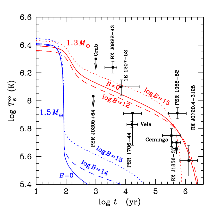
Figure 12: Effective surface temperature (as seen by distant observer) versus neutron star age for assumed mass $1.3M_{\odot}$ and $1.5M_{\odot}$. The dots with error bars show estimates of neutron star ages and effective temperatures from various observations; the dots with errors indicate observational upper limits. The different curves show the cooling of neutron stars with iron envelope for different magnetic field strengths (log $B$ in Gauss). From Chabrier, Saumon & Potekhin (2006).

6.4 Outermost Envelopes

The outermost layer of a neutron star is of great importance since it mediates the emergent radiation from the stellar surface to the observer. The chemical composition of this layer is unknown. The surface of a fully catalyzed neutron star is expected to consist of ⁵⁶Fe formed at the star’s birth, although C, O may also be present. This may be the case for young radio pulsars that have not accreted any gas. Once the neutron star accretes material, or has gone through a phase of accretion, either during supernova fallback, or from the interstellar medium or from a binary companion, the surface composition can be quite different. A H layer is expected even if a small amount of fallback/accretion occurs after neutron star formation. A He layer results if H is completely burnt out. The atmosphere composition may also be affected by the (slow) nuclear burning on the NS surface layer (Chang, Arras & Bildsten 2004) and by the bombardment of high-energy particles on the surface (Thompson & Beloborodov 2005).

Despite the uncertainties in the surface composition mentioned in the last paragraph, a great simplification arises due to the efficient gravitational separation of light and heavy elements. As an example, consider a trace amount of ions (with charge number $Z_{i}$ and mass number $A_{i}$) embedded in the ionized hydrogen plasma (with the electron number density $n_{e}$) of a neutron star atmosphere. The downward drift speed of the ion relative to the H plasma is $v_{\rm drift}\simeq g\,t_{f}$, where $g$ is the gravitational acceleration. The friction timescale $t_{f}$ can be estimated from ${A_{i}m_{p}/t_{f}}\approx n_{e}m_{p}\sigma_{pi}v_{p}$, where the ion-proton Coulomb collision cross-section is $\sigma_{pi}\sim(Z_{i}e^{2}/k_{B}T)^{2}\ln\Lambda$ (here $\ln\Lambda$ is the Coulomb logarithm), and the thermal velocity of the proton is $v_{p}\sim(k_{B}T/m_{p})^{1/2}$. This gives

$$t_{f}\sim{A_{i}\over Z_{i}^{2}\ln\Lambda}{m_{p}^{1/2}(k_{B}T)^{3/2}\over e^{4}n_{e}}.$$ (135)

Using typical parameters ($g\sim 2\times 10^{14}$ cm s^-2, $T\sim 10^{6}$ K, $n_{e}\sim 10^{24}$ cm^-3), we find that the drift speed is of order $10\,(A_{i}/Z_{i}^{2}\ln\Lambda)$ cm s^-1. The timescale for gravitational settling over the pressure scale height $H\sim k_{B}T/(m_{p}g)$ is of order a second. Thus the lightest elements, H and He, if present, are the most important chemical species in the outermost layer of the star.

The hydrogen envelope of a neutron star may assume different forms, depending on the temperature and magnetic field. For “modest” field strengths ($B\mathrel{\raise 1.29167pt\hbox{$<$}\mkern-14.0mu\lower 2.58334pt\hbox{$\sim$}}{\rm a~{}few}\times 10^{13}$ G) and temperatures ($T\mathrel{\raise 1.29167pt\hbox{$>$}\mkern-14.0mu\lower 2.58334pt\hbox{$\sim$}}10^{5}$ K), conditions satisfied by most observable neutron stars, the atmosphere is largely nondegenerate, and consists mainly of ionized hydrogen, H atoms and small H_N molecules, and the condensed phase can be neglected in the photosphere. As density increases, the matter gradually transform into a degenerate Coulomb plasma (see above). The atmosphere (with density $\rho\sim 10^{-3}-10^{4}$ g cm^-3) constitutes a non-ideal, partially ionized, Coulomb plasma. An important issue concerns the ionization equilibrium of atoms in such a plasma. This is nontrivial because in a strong magnetic field, an atom cannot move free across the field, and there is strong coupling between the internal atomic structure and the center-of-mass motion (see §3.1). Lai & Salpeter (1995) gave an approximate analytic solution for a limited magnetic-field–temperature–denisty regime (see also Khersonskii 1987; Pavlov & Meszaros 1993). To date the most complete treatment of the equation of state (including Saha equilibrium) of partially ionized hydrogen plasma is that of Potekhin et al. (1999) (for $10^{11}$ G$\mathrel{\raise 1.29167pt\hbox{$<$}\mkern-14.0mu\lower 2.58334pt\hbox{$\sim$}}B\mathrel{\raise 1.29167pt\hbox{$<$}\mkern-14.0mu\lower 2.58334pt\hbox{$\sim$}}10^{13}$ G) and Potekhin & Chabrier (2004) (for $10^{13}$ G$\mathrel{\raise 1.29167pt\hbox{$<$}\mkern-14.0mu\lower 2.58334pt\hbox{$\sim$}}B\mathrel{\raise 1.29167pt\hbox{$<$}\mkern-14.0mu\lower 2.58334pt\hbox{$\sim$}}10^{15}$ G). They used the numerical energy levels and fitting formulae of a moving H atom as obtained by Potekhin (1994,1998), and their free energy model takes into account the Coulomb plasma nonideality, the interactions of bound species with one another and with the electrons and protons. Ionization equilibrium is given by minimization of the free energy with respect to particle numbers under the stoichiometric constraints (keeping the volume and the total number of free and bound protons constant). The derivatives of the free energy with respect to $\rho$ and $T$ and their combinations provide the other thermodynamic functions. Figure 13 shows the domains of partial ionization in the $\rho-T$ plane for different values of $B$. The higher $B$, the greater $T$ at which the bound species are important. The calculated atomic fractions are needed to obtain the radiative opacities in the atmosphere. Note that the Potekhin et al. model becomes less reliable at relatively low $T$ where larger molecules can be important (Lai 2001). Generally, this occurs within the $\rho-T$ domain where $x_{\mathrm{H}}\mathrel{\raise 1.29167pt\hbox{$>$}\mkern-14.0mu\lower 2.58334pt\hbox{$\sim$}}0.1$ (i.e., to the left of the solid lines in Fig. 13).

Figure 13: Domains of partial ionization in the $\rho-T$ plane for $B=10^{12}$, $10^{13}$ and $10^{14}$ G. The contours delimit the domains where the atomic fraction $x_{\mathrm{H}}<0.1$% (to the right of the dotted lines), 0.1%$<x_{\mathrm{H}}<1$% (between the dashed and dotted lines), 1%$<x_{\mathrm{H}}<10$% (between the solid and dashed lines) or $x_{\mathrm{H}}>10$% (to the left of the solid lines). From Potekhin et al. (2006).

For sufficiently strong magnetic fields and/or low temperatures, the hydrogen layer may be in a condensed, metallic form, since the binding energy of the condensed hydrogen increases as a power-law function of $B$, while the binding energies of atoms and small molecules increase only logarithmically. Lai & Salpeter (1997) studied the phase diagram of H under different conditions and showed that in strong magnetic fields, there exists a critical temperature $T_{\rm crit}$ below which a phase transition from gaseous to condensed state occurs, with $kT_{\rm crit}$ about $10\%$ of the cohesive energy of the condensed hydrogen. Thus, $T_{\rm crit}\sim 8\times 10^{4},\,5\times 10^{5},\,10^{6}$ K for $B=10^{13},\,10^{14},\,5\times 10^{14}$ G (Lai 2001). An analogous “plasma phase transition” was also obtained in an alternative thermodynamic model for magnetized hydrogen plasma (Potekhin et al. 1999). While this model is more restricted than Lai & Salpeter (1997) in that it does not include H_N molecules, it treats more rigorously atomic motion across the strong $B$ field and Coulomb plasma nonideality. In the Potekhin et al. model, the density of phase separation is roughly the same as in Lai & Salpeter (1997), i.e., $\rho_{s,0}\sim 10^{3}\,B_{12}^{6/5}$ g cm^-3 [see Eq. (31)], but the critical temperature is several times higher. Thus, although there is a factor of a few uncertainty in $T_{\rm crit}$, it is almost certain that for $T\mathrel{\raise 1.29167pt\hbox{$<$}\mkern-14.0mu\lower 2.58334pt\hbox{$\sim$}}T_{\rm crit}/2$, the H surface of a neutron star is in the form of the condensed metallic state, with negligible vapor above it. The radiative property of such condensed phase is discussed in §8.

For heavy elements such as Fe, detailed study of the phase diagram is not available since our current knowledge of the various states/phases in strong magnetic fields is not as complete as for H (see §3.4). Calculations so far have shown that at $B=10^{12}-10^{13}$ G, a linear chain is unbound relative to individual atoms for $Z\mathrel{\raise 1.29167pt\hbox{$>$}\mkern-14.0mu\lower 2.58334pt\hbox{$\sim$}}6$, and thus chain-chain interactions play an important role in determining whether 3D zero-pressure condensed matter is bound or not. For larger field strengths, $B\buildrel>\over{\sim}10^{14}(Z/26)^{3}$ G, a linear chain becomes bound (Medin & Lai 2006). If the condensed Fe is unbound with respect to the Fe atom, then the outermost Fe layer of the neutron star is characterized by gradual transformation from nondegenerate gas at low densities, which includes Fe atoms and ions, to degenerate plasma as the pressure (or column density) increases. On the other hand, even a weak cohesion of the Fe condensate can give rise to a phase transition at sufficiently low temperatures. Crude numerical results by Jones (1986) together with approximate scaling relations suggest an upper limit of the cohesive energy (for $Z\mathrel{\raise 1.29167pt\hbox{$>$}\mkern-14.0mu\lower 2.58334pt\hbox{$\sim$}}10$) $Q_{s}\mathrel{\raise 1.29167pt\hbox{$<$}\mkern-14.0mu\lower 2.58334pt\hbox{$\sim$}}Z^{9/5}B_{12}^{2/5}$ eV. Thus for Fe, the critical temperature for phase transition $T_{\rm crit}\mathrel{\raise 1.29167pt\hbox{$<$}\mkern-14.0mu\lower 2.58334pt\hbox{$\sim$}}0.1Q_{s}/k\mathrel{\raise 1.29167pt\hbox{$<$}\mkern-14.0mu\lower 2.58334pt\hbox{$\sim$}}10^{5.5}B_{12}^{2/5}$ K.

The iron surface layers of magnetic neutron stars can also studied using Thomas-Fermi type models (e.g., Fushiki, Gudmundsson & Pethick 1989; Thorolfsson et al. 1998). While these models are too crude to determine the cohesive energy of the condensed matter, they provide a useful approximation to the gross properties of the neutron star surface layer. At zero temperature, the pressure is zero at a finite density which increases with increasing $B$. This feature is qualitatively the same as in the uniform electron gas model. Neglecting the exchange-correlation energy and the nonuniformity correction, we can write the pressure of a zero-temperature uniform electron gas as

$$P=P_{e}-{3\over 10}\left({4\pi\over 3}\right)^{1/3}\!\!\!\!(Ze)^{2}\!\left({\rho\over Am_{p}}\right)^{4/3},$$ (136)

where the first term is given by Eq. (119) [or by Eq. (129) in the strong field, degenerate limit], and the second term results from the Couloumb interactions among the electrons and ions. Setting $P=0$ gives the condensation density $\rho_{s,0}$ as in Eq. (31). At finite temperatures, the pressure does not go to zero until $\rho\rightarrow 0$, i.e., an atmosphere is present. Note that the finite-temperature Thomas-Fermi model only gives a qualitative description of the dense atmsophere; important features such as atomic states and ionizations are not captured in such a model.

7 Neutron Star Magnetic Field Evolution

Magnetic field is perhaps the single most important quantity that determines the various observational manifestations of neutron stars. Thus it is natural that a large amount of work has been devoted to the study of neutron star magnetic field evolution. Recent reviews include Bhattacharya & Srinivasan (1995), Ruderman (2004), Reisenegger et al. (2005).

7.1 Observations

As discussed in §1, with a few exceptions, our current knowledge of neutron star magnetic fields are largely based on indirect inferences:

(i) For radio pulsars, of which about 1600 are known today (see Manchester 2004), the period $P$ and period derivative $\dot{P}$ can be measured by timing the arrivals of radio pulses. If we assume that the pulsar spindown is due to magnetic dipole radiation, we obtain an estimate of the neutron star surface field $B$ [see Eq. (1)]. For most radio pulsars, the inferred $B$ lies in the range of $10^{11}-10^{14}$ G. For a smaller population of older, millisecond pulsars, $B\sim 10^{8-9}$ G – Such field reduction is thought to be related to the recycling process that turns a dead pulsar into an active, millisecond pulsar.

(ii) For Anomalous X-ray pulsars and Soft Gamma Repeaters (Woods & Thompson 2005), superstrong magnetic fields ($B\sim 10^{14}-10^{15}$ G) are again inferred from the measured $P$ (in the range $5-12$ s) and $\dot{P}$ (based on X-ray timing study) and the assumption that the spin-down is due to the usual magnetic dipole radiation or Alfvén wave emission. In addition, strong theoretical arguments have been put forward (Thompson & Duncan 1995,1996,2001) which suggest that a superstrong magnetic field is needed to explain various observed properties of AXPs and SGRs (e.g., energetics of SGR bursts/flares, including the spectacular giant flares from three SGRs: the March 5 1979 flare of SGR 0525-66 with energy $E\mathrel{\raise 1.29167pt\hbox{$>$}\mkern-14.0mu\lower 2.58334pt\hbox{$\sim$}}6\times 10^{44}$ erg, the August 27 1998 flare from SGR 1900+14 with $E\mathrel{\raise 1.29167pt\hbox{$>$}\mkern-14.0mu\lower 2.58334pt\hbox{$\sim$}}2\times 10^{44}$ erg, and the December 27 2004 flare from SGR 1806-20 with $E\sim 4\times 10^{46}$ erg; quiescent luminosity $L_{x}\sim 10^{34-36}$ erg/s, much larger than the spindown luminosity $I\Omega\dot{\Omega}$) (see §10). Tentative detections of spectral features during SGR/AXP bursts have been reported in several systems (e.g., Gavriil et al. 2003; Ibrahim et al. 2003; Rea et al. 2003), which, when interpreted as proton cyclotron lines, imply $B\sim 10^{15}$ G.

(iii) For a number of thermally emitting neutron stars (“dim isolated neutron stars”), spectral features with energy $0.2-1$ keV have been detected (see §8.1). While the identification of these features is unclear, if one assumes that they are due to proton cyclotron resonance or atomic transitions in light elements, one would infer $B\sim 10^{13}-10^{14}$ G.

(iv) For about a dozen accreting X-ray pulsars in binary systems, electron cyclotron features have been detected, implying $B\sim 10^{12}-10^{13}$ G (see §1). For many other X-ray pulsars with no detectable cyclotron features, we can use the measured spin period together with theoretical ideas of spin equilibrium (i.e., spinup due to accretion of matter is balanced by magnetic braking – loss of stellar angular momentum via magnetic fields) to estimate the surface magnetic field of the neutron star. For the $\sim 100$ neutron stars in high-mass X-ray binaries, this typically gives $B\sim 10^{12}$ G (e.g., Bildsten et al. 1997). In the last few years, half a dozen or so accreting millisecond pulsars have been discovered (e.g., Chakrabarty 2005), with the estimated field strength $B\sim 10^{9}$ G — these systems are thought to be neutron stars undergoing the recycling process.

Several lines of observations/arguments point toward the possibility of an evolving magnetic fields in neutron stars.

(i) From the discussion above, it appears that young neutron stars have strong magnetic fields $\sim 10^{11}-10^{15}$ G (most radio pulsars, magnetars, high-mass X-ray binaries), whereas old neutron stars have weak fields $\mathrel{\raise 1.29167pt\hbox{$<$}\mkern-14.0mu\lower 2.58334pt\hbox{$\sim$}}10^{9}$ G (millisecond pulsars, low-mass X-ray binaries). If these two groups have an evolutionary connection, then the field must be significantly reduced on timescale of $10^{9}$ yr. Most likely, this reduction is associated with the accretion process that recycled the neutron star.

(ii) Magnetic field evolution in isolated pulsars has long been studied using the statistical distribution of pulsars on the $P-\dot{P}$ diagram, as well as pulsars’ spatial and velocity distributions. Such study probes field evolution on the timescale of the ages of radio pulsars ($\mathrel{\raise 1.29167pt\hbox{$<$}\mkern-14.0mu\lower 2.58334pt\hbox{$\sim$}}10^{7}$ yr). Unfortunately, the conclusions of such population study have often been conflicting. For example, Narayan & Ostriker (1990) and Gonthier et al. (2004) suggested that field decay occurs on timescale $\mathrel{\raise 1.29167pt\hbox{$<$}\mkern-14.0mu\lower 2.58334pt\hbox{$\sim$}}5$ Myr. Similar studies by Bhattacharya et al. (1992), Lorimer et al. (1997), Faucher-Giguéré & Kaspi (2006) found no evidence for field decay during the radio pulsar lifetime, implying a decay time constant $\mathrel{\raise 1.29167pt\hbox{$>$}\mkern-14.0mu\lower 2.58334pt\hbox{$\sim$}}100$ Myr. Such divergent results illustrate the difficulties of controlling various systematic uncertainties (e.g. selection effects, luminosity evolution law, dependence of beaming fraction on period) in pulsar population studies.

(iii) Magnetar emission is most likely powered by magnetic energy, implying the dissipation of superstrong magnetic fields (see Thompson & Duncan 1995,1996; Woods & Thompson 2005).

(iv) One explanation for the “anomalous” braking indices $n<3$ in young pulsars is that their magnetic dipole field increases with time (but see Melatos 1997). It has also been pointed out that following each pulsar glitch, the apparent magnetic field $\propto\sqrt{P\dot{P}}$) increases, which might imply that some pulsars (Crab and Vela), may evolve into magnetars (Lyne 2004; Lin & Zhang 2004). Since many AXPs and SGRs are observed to be associated with supernova remnants or clusters of massive stars, most magnetars are expected to be younger than radio pulsars, rather than the other way around.

7.2 Origin of Neutron Star Magnetic Field

The magnetic fields of neutron stars were most likely already present at birth. The traditional fossil field hypothesis suggests that the magnetic field is inherited from the progenitor, with magnetic flux conserved and field amplified ($B\propto R^{-2}$) during core collapse. In the case of magnetic white dwarfs (with measured fields in the range $\sim 3\times 10^{4}-10^{9}$ G), there is strong evidence that the fields are the remnants from a main-sequence phase (Ap/Bp stars, with $B\sim 200$ G –25 kG) (see, e.g., Ferrario & Wichramasinghe 2005). Neutron stars descend from main-sequence stars with mass $\mathrel{\raise 1.29167pt\hbox{$>$}\mkern-14.0mu\lower 2.58334pt\hbox{$\sim$}}8M_{\odot}$ (i.e., O and early B stars). Only recently have the large-scale magnetic fields (with $B\sim 1$ kG) of O stars been detected (in two stars so far; see Donati et al. 2006). It is interesting that the magnetic flux of such O stars $\Phi\sim 10^{5}\pi R_{\odot}$ G (for $R\sim 10R_{\odot}$; of course, not all of this flux threads the inner $1.4M_{\odot}$ core) is of the same order of magnitude as the flux of a $10^{15}$ G neutron star ($R\sim 10^{-5}R_{\odot}$) as well as the fluxes of the most strongly magnetic Ap/Bp stars and white dwarfs. It is also of interest to note that magnetic white dwarfs ($B\mathrel{\raise 1.29167pt\hbox{$>$}\mkern-14.0mu\lower 2.58334pt\hbox{$\sim$}}1$ MG) tend to be more massive (mean mass $\sim 0.93M_{\odot}$) than their non-magnetic counterparts (mean mass $\sim 0.6M_{\odot}$). Since white dwarfs with $M\mathrel{\raise 1.29167pt\hbox{$>$}\mkern-14.0mu\lower 2.58334pt\hbox{$\sim$}}0.7M_{\odot}$ and neutron stars form exclusively from the material that belongs to the convective core of a main-sequence star (Reisenegger 2001), this suggests that the magnetic field may be generated in the convective core of the main-sequence progenitor. It has also been suggested that magnetized neutron stars could be produced, in principle, by accretion-induced collapse of magnetic white dwarfs (Usov 1992).

Alternatively, it has been argued that magnetic field may be generated by a convective dynamo in the first $\sim 10$ seconds of a proto-neutron star (Thompson & Duncan 1993). In principle, the maximum field achievable is either $B\sim(4\pi\rho)^{1/2}v_{\rm con}\sim 4\times 10^{15}$ G (for convective eddy speed $v_{\rm con}\sim 10^{3}$ km s^-1) or $B\sim(4\pi\rho)^{1/2}R\Delta\Omega\sim 2\times 10^{17}$ G [for differential rotation $\Delta\Omega\sim 2\pi/(1~{}{\rm ms})$]. How much dipole field can be generated is more uncertain. It could be that a large-scale field of $\sim 10^{15}$ G is generated if the initial spin period of the neutron star is comparable to the convective turnover time ($\sim H_{p}/v_{\rm con}\sim 1$ ms for pressure scale height of 1 km), whereas in general only a small-scale ($\sim H_{p}$) field is produced, resulting in mean field of order $10^{12}-10^{13}$ G typical of radio pulsars. We note that studies of presupernova evolution of massive stars, including magnetic fields, typically find that a newly formed neutron star has rotation rate appreciably slower than the breakup rate (Heger et al. 2005).

In either the fossil field or dynamo scenario, the magnetic field of a proto-neutron star is likely “messy” and unstable. Before the crust forms (around $100$ s afetr collapse), the field will evolve on the Alfven crossing time $t_{A}\sim(4\pi\rho)^{1/2}R/B$ ($\sim 0.1$ s for $B\sim 10^{15}$ G) into a stable configuration in which a poloidal field coexists with a toroidal field of the same order of magnitude (see Braithwaite & Spruit 2006).

Gradual field generation due to a thermomagnetic effect in the crust has been discussed (Urpin & Yakovlev 1980; Blandford et al. 1983; Wiebicke & Geppert 1996), but it seems unlikely to be capable of producing large-scale fields stronger than $10^{12}$ G.

7.3 Physics of Field Evolution in Isolated Neutron Stars

The magnetic field in a neutron star evolves through a series of quasi-equilibrium states, punctuated by the release of elastic stress in the crust and hydrodynamic motions in its liquid core. The physics of the quasi-equilibrium field evolution was discussed by Goldreich & Reisenegger (1992) (see also Reisenegger et al. 2005). The bulk region of a neutron star comprises a liquid core of mostly neutrons with a small fraction ($Y_{e}\sim{\rm a~{}few}\%$) of protons and electrons. The medium is stably stratified due to the $Y_{e}$ gradient, thus the magnetic field cannot force the bulk neutron fluid to move (e.g. due to buoyancy) unless $B^{2}/(8\pi)\mathrel{\raise 1.29167pt\hbox{$>$}\mkern-14.0mu\lower 2.58334pt\hbox{$\sim$}}Y_{e}P$ (or $B\mathrel{\raise 1.29167pt\hbox{$>$}\mkern-14.0mu\lower 2.58334pt\hbox{$\sim$}}10^{17}$ G) or the fluid can change its composition as it rises (which takes place on a timescale longer than the neutrino cooling time for $B\mathrel{\raise 1.29167pt\hbox{$<$}\mkern-14.0mu\lower 2.58334pt\hbox{$\sim$}}10^{17}$ G). The magnetic field evolves according to

$${\partial{\bf B}\over\partial t}=-\nabla\times\left({c^{2}\over 4\pi\sigma}\nabla\times{\bf B}\right)+\nabla\times\left(-{{\bf j}\over n_{e}e}\times{\bf B}\right)+\nabla\times\left({\bf v}_{a}\times{\bf B}\right),$$ (137)

where the three terms on the right-hand side represent three different effects:

(i) The first term represents Ohmic diffusion of the magnetic field ($\sigma$ is the zero-field conductivity defined by ${\bf j}=\sigma{\bf E}$), with timescale

$$t_{\rm Ohmic}\sim{4\pi\sigma L^{2}\over c^{2}}$$ (138)

for fields which vary on lengthscale $L$. In the core, the conductivity is large since all the particles are degenerate, leading to $t_{\rm Ohmic}\sim 2\times 10^{11}(L_{\rm km}/T_{8})^{2}(\rho/\rho_{\rm nuc})^{3}$ yr (Baym, Pethick & Pines 1969), where $\rho_{\rm nuc}=2.8\times 10^{14}$ g cm^-3, $L_{\rm km}=L/(1~{}{\rm km})$. Of course, currents which are confined to the crust would have a much shorter decay time (e.g., Sang & Chanmugam 1987; Cumming et al. 2004).

(ii) The second term describes advection of the field by Hall drift: The magnetic field is carried by the electron fluid, which drifts with respect to the ions with velocity ${\bf v}_{e}=-{\bf j}/(n_{e}e)$. This term is non-dissipative, but can change the field structure on timescale

$$t_{\rm Hall}\sim{4\pi n_{e}eL^{2}\over cB}\sim 5\times 10^{8}{L_{\rm km}^{2}\over B_{12}}\left({\rho\over\rho_{\rm nuc}}\right)~{}{\rm yr}.$$ (139)

Goldreich & Reisenegger (1992) suggested that the nonlinear Hall term may give rise to a turbulent cascade to small scale, thus enhancing the Ohmic dissipation rate of the field. This “Hall cascade” has been confirmed by recent simulations of electron MHD turbulence (also known as whistler turbulence; see Cho & Lazarian 2004). Several studies have also demonstrated magnetic energy transfer between different scales (e.g., Urpin & Shalybkov 1999; Hollerbach & Rüdiger 2002). A specific example of the Hall-drift enhanced Ohmic dissipation can be seen by considering a purely toroidal field (see Reisenegger et al. 2005): In this case, the evolution equation for the field reduces to the Burgers equation (see also Vainshtein et al. 2000), where the field tends to develop a cusp (and the associated current sheet) and fast Ohmic decay. Recently, Rheinhardt & Geppert (2002) and Rheinhardt et al. (2004) discussed a “Hall drift instability” that can lead to nonlocal transfer of magnetic energy to small scales, leading to enhanced crustal field dissipation.

(iii) The third term describes ambipolar diffusion, which involves a drift of the combined magnetic field and the bulk electron-proton fluid relative to the neutrons. The drift velocity ${\bf v}_{a}$ is determined by force balance $m_{p}{\bf v}_{a}/\tau_{pn}={\bf f}_{B}-\nabla(\Delta\mu)$, where $\tau_{pn}$ is the proton-neutron collision time, ${\bf f}_{B}={\bf j}\times{\bf B}/(cn_{p})$ is the magnetic force per proton-electron pair, and $\nabla(\Delta\mu)$ (with $\Delta\mu=\mu_{p}+\mu_{e}-\mu_{n}$) is the net pressure force due to imbalance of $\beta$-equilibrium (Goldreich & Reisenegger 1992). There are two modes of ambipolar diffusion: The solenoidal mode ($\nabla\cdot{\bf v}_{a}=0$) is noncompressive, and does not perturb $\beta$-equilibrium, thus ${\bf v}_{a}=\tau_{pn}પ\tau_{pn}{\bf f}_{B}/m_{p}$, and the associated diffusion time $t_{\rm Amb}^{\rm s}\sim L/v_{a}$ is

$$t_{\rm Amb}^{\rm s}\sim{4\pi n_{p}m_{p}L^{2}\over\tau_{pn}B^{2}}\sim 3\times 10^{9}\,{T_{8}^{2}L_{\rm km}^{2}\over B_{12}^{2}}~{}{\rm yr},$$ (140)

where we have used $n_{p}\simeq 0.05\rho/m_{p}$ and $\tau_{pn}\simeq 2\times 10^{-17}T_{8}^{-2}(\rho/\rho_{\rm nuc})^{1/3}$ s. The irrotational mode ($\nabla\times{\bf v}_{a}=0$) is compressive, and is impeded by chemical potential gradients $\nabla(\Delta\mu)$, and is possible only if weak interaction re-establishes $\beta$-equilibrium during the drift. This gives a timescale $t_{\rm Amb}^{\rm ir}\sim t_{\rm cool}/B_{17}^{2}\sim 5\times 10^{15}T_{8}^{-6}B_{12}^{-2}$ yr (where $t_{\rm cool}$ is the neutrino cooling time and modified URCA rate has been used). Like Ohmic decay, ambipolar diffusion is dissipative, which leads to heating of the core and deep crust of a magnetar; this may be the power source for the persistent X-ray emission of magnetars (Thompson & Duncan 1996; Heyl & Kulkarni 1998; Arras et al. 2004; see §10).

In addition the the “steady” field evolution discussed above, crust fracture can also lead to sudden change of the magnetic field (Thompson & Duncan 1996). The crust has a finite shear modulus $\mu$, and when the yield strain $\theta_{\rm max}$ is exceeded the lattice will fracture. The characteristic yield field strength is of order $\sim(4\pi\theta_{\rm max}\mu)^{1/2}=2\times 10^{14}(\theta_{\rm max}/10^{-3})^{1/2}$ G. For example, Hall drift of the magnetic field causes the stresses in the crust to build up, and irregularities in the field can be damped quickly by crustal yielding – this may be responsible for magnetar bursts (Thompson & Duncan 1995; see §10).

7.4 Accretion-Induced Field Reduction

The weak ($10^{8}-10^{9}$ G) magnetic fields found in millisecond pulsars and low-mass X-ray binaries have long led to the suggestion that the dipole field is reduced during accretion, perhaps through diamagnetic screening of the magnetic flux by the accreted plasma (e.g., Bisnovati-Kogan & Komberg 1975; Shibazaki et al. 1989; Romani 1990). Exactly how this is achieved (if at all) is not clear, and a number of idealized problems have been studied. To give some recent examples: Cumming et al. (2001) considered a 1D model in which matter accretes onto horizontal field lines, and showed that inward field advection can compete with outward Ohmic diffusion only when the accretion rate is larger than $10\%$ of the Eddington rate; Payne & Melatos (2004) constructed global hydromagnetic equilibrium sequence of a neutron star accreting at the magnetic poles (see also Melatos & Phinney 2001); Lovelace et al. (2005) considered a model in which the magnetic field is screened by the current in the infalling plasma outside the star. In any case, it is not clear that such field burial is effective or permanent, as the field tends to resurface due to various instabilities (e.g. buoyancy). If the original field is sustained by currents in the crust, then accelerated Ohmic decay due to accretion-induced heating may be a viable mechanism (e.g., Urpin & Geppert 1995; Konar & Bhattacharya 1998).

A different type of accretion-induced field reduction mechanism relies on the interaction between superfluid neutron vortices and superconducting magnetic fluxoids in the stellar interior (see Srinivasan et al. 1990). When the star spins up, the fluxoids are dragged together with the vortices toward the rotation axis, which leads to a reduction of the effective dipole moment even though the local field strength at the magnetic poles actually increases (Ruderman 1991a,b). Various observational consequences of such vortices migration have been reviewed by Ruderman (2004).

8 Thermal Radiation from Magnetized Neutron Stars

8.1 Observational Background

It has long be recognized that thermal, surface emission from isolated neutron stars (NSs) can potentially provide invaluable information on the physical properties and evolution of NS (equation of state at super-nuclear densities, superfluidity, cooling history, magnetic field, surface composition, different NS populations, etc. See, e.g., Prakash et al. 2001; Yakovlev & Pethick 2004 for review). In the last few years, considerable observational resources (e.g. Chandra and XMM-Newton) have been devoted to such study. For example, the spectra of a number of radio pulsars (e.g., PSR B1055-52, B0656+14, Geminga and Vela) have been observed to possess thermal components that can be attributed to emission from NS surfaces and/or heated polar caps (e.g., Becker & Pavlov 2002). Phase-resolved spectroscopic observations are becoming possible, revealing the surface magnetic field geometry and emission radius of the pulsar (e.g., Caraveo et al. 2004; De Luca et al. 2005; Jackson & Halpern 2005). Chandra has also uncovered a number of compact sources in supernova remnants with spectra consistent with thermal emission from NSs (see Pavlov et al. 2003), and useful constraints on NS cooling physics have been obtained (e.g., Slane et al. 2002; Yakovlev & Pethick 2004).

Surface X-ray emission has also been detected from a number of soft gamma-ray repeaters (SGRs) and anomalous X-ray pulsars (AXPs) — these are thought to be magnetars, whose radiation is powered by the decay of superstrong ($B\mathrel{\raise 1.29167pt\hbox{$>$}\mkern-14.0mu\lower 2.58334pt\hbox{$\sim$}}10^{14}$ G) magnetic fields (see Thompson & Duncan 1995,1996; Woods & Thompson 2005). Fits to the quiescent magnetar spectra with blackbody or with crude atmosphere models indicate that the thermal X-rays can be attributed to magnetar surface emission at temperatures of (3–7) $\times 10^{6}$ K (see, e.g., Juett et al 2002; Tiengo et al. 2002; Patel et al. 2003; Kulkarni et al. 2003; Tiengo et al. 2005). One of the intriguing puzzles is the absence of spectral features (such as ion cyclotron line around 1 keV for typical magnetar field strengths) in the observed thermal spectra. Clearly, detailed observational and theoretical studies of surface emission can potentially reveal much about the physical conditions and the nature of magnetars.

Also of great interest are the seven or so isolated, radio-quiet NSs (so-called “dim isolated NSs”; see Haberl 2005). These NSs share the common property that their spectra appear to be entirely thermal, indicating that the emission arises directly from the NS atmospheres, uncontaminated by magnetospheric processes. Thus they offer the best hope for inferring the precise values of the temperature, surface gravity, gravitational redshift and magnetic field strength. The true nature of these sources, however, is unclear at present: they could be young cooling NSs, or NSs kept hot by accretion from the ISM, or magnetars and their descendants (e.g., van Kerkwijk & Kulkarni 2001, Mori & Ruderman 2003; Haberl 2005; Kaspi et al. 2005). Given their interest, these isolated NSs have been intensively studied by deep Chandra and XMM-Newton observations. While the brightest of these, RX J1856.5-3754, has a featureless spectrum remarkably well described by a blackbody (Drake et al. 2002; Burwitz et al. 2003), absorption lines/features at $E\simeq 0.2$–$2$ keV have recently been detected from at least four sources, including 1E 1207.4-5209 (0.7 and 1.4 keV, possibly also 2.1, 2.8 keV; Sanwal et al. 2002; DeLuca et al. 2004; Mori et al. 2005), RX J1308.6+2127 (0.2-0.3 keV; Haberl et al. 2003), RX J1605.3+3249 (0.45 keV; van Kerkwijk et al. 2004) and RX J0720.4$-$3125 (0.27 keV; Haberl et al. 2004), and possibly two additional sources (see Zane et al. 2005). The identifications of these features, however, remain uncertain, with suggestions ranging from electron/ion cyclotron lines to atomic transitions of H, He or mid-Z atoms in a strong magnetic field (Ho & Lai 2004; Pavlov & Bezchastnov 2005; Mori et al. 2005). These sources also have different X-ray light curves: e.g., RX J1856.5-3754 and RX J1605+3249 show no variability (pulse fraction $\mathrel{\raise 1.29167pt\hbox{$<$}\mkern-14.0mu\lower 2.58334pt\hbox{$\sim$}}1$-$3\%$); RX J0720-3125 shows a single-peaked $P=3.39$ s pulsation of amplitude $\sim 11\%$, with the spectral hardness and line width varying with the pulse phase; RX J 1308+2127 has a double-peaked pulsation with $P=10.3$ s and amplitude $\sim 18\%$. Another puzzle concerns the optical emission: For at least four of these sources, the optical counterparts have been identified, but the optical flux is larger (by a factor of $4$-$10$) than the extrapolation from the black-body fit to the X-ray spectrum (see Haberl 2005).

The preceding paragraphs highlight the great observational progress made in recent years on the study of NS surface emission. These observations can potentially tell us much about the physics and astrophysics of NSs. Future X-ray telescopes (Constellation-X and XEUS) will have great capability of studying NS surface emission. In order to properly interpret the current and future observations, it is crucial to have a detailed understanding of the radiative properties of the outer layers of NSs in the presence of intense magnetic fields, and to model the emergent thermal radiation spectra from the NS.

8.2 Modeling Neutron Star Surface Radiation

Thermal radiation from a magnetized NS is mediated by the thin atmospheric layer (with scale height $0.1$–$10$ cm and density $\sim 10^{-3}$–$10^{4}$ g cm^-3) that covers the stellar surface. The physical properties of the atmosphere, such as the chemical composition, equation of state, and especially the radiative opacities, directly determine the characteristics of the thermal emission. While the surface composition of the NS is unknown, a great simplification arises due to the efficient gravitational separation of light and heavy elements (see §6.4). The strong magnetic field makes the atmospheric plasma anisotropic and birefringent. If the surface temperature is not too high, atoms and molecules may form in the atmosphere. Moreover, if the magnetic field is sufficiently strong, the NS envelope may transform into a condensed phase with very little gas above it (§6.4). A superstrong magnetic field will also make some quantum electrodynamics (QED) effects (e.g., vacuum polarization) important in calculating the surface radiation spectrum (see §8.3 below).

The first models of zero-field NS atmospheres were constructed by Romani (1987). Further works used improved opacity and equation of state data from the OPAL project for pure hydrogen, helium and iron compositions (Rajagopal & Romani 1996; Zavlin et al. 1996; Gänsicke et al. 2002; Pons et al. 2002). These models may be applicable to weakly magnetized ($B\mathrel{\raise 1.29167pt\hbox{$<$}\mkern-14.0mu\lower 2.58334pt\hbox{$\sim$}}10^{8}$ G) NSs. So far most studies of magnetic NS atmospheres have focused on hydrogen and moderate field strengths of $B\sim 10^{12}$–$10^{13}$ G (e.g., Shibanov et al. 1992; Zane et al. 2000; Zavlin & Pavlov 2002). These models take into account the transport of different photon modes through a mostly ionized medium. The opacities adopted in the models include free-free transitions and electron scattering. However, since a strong magnetic field greatly increases the binding energies of bound species (see §3), atoms, molecules, and other bound states may have appreciable abundances in the atmosphere (see §6.4). Thus these magnetic atmosphere models are expected to be valid only for relatively high temperatures ($T\mathrel{\raise 1.29167pt\hbox{$>$}\mkern-14.0mu\lower 2.58334pt\hbox{$\sim$}}{\rm a~{}few}\times 10^{6}$ K) where hydrogen is almost completely ionized. As the magnetic field increases, we expect these models to break down at even higher temperatures as bound atoms, molecules and condensate become increasingly important. Models of magnetic iron atmospheres (with $B\sim 10^{12}$ G) were studied by Rajagopal et al. (1997). Because of the complexity in the atomic physics and radiative transport, these Fe models are necessarily crude.

NS atmospheres with superstrong ($B\mathrel{\raise 1.29167pt\hbox{$>$}\mkern-14.0mu\lower 2.58334pt\hbox{$\sim$}}10^{14}$ G) magnetic field have been studied recently (Ho & Lai 2001,2003,2004; Özel 2001; Zane et al. 2001). Currently most models treat ionized H and He atmospheres, and include full angle-dependent transport of the photon polarization modes and ion cyclotron resonance in the opacity. The effect of vacuum polarization has been studied, and is found to be important for determining the thermal spectra and polarizations of magnetized NSs (see §8.3). Recently, NS atmosphere models that include self-consistent treatment of the thermodynamics and opacities of bound H atoms in strong magnetic fields were constructed (see §8.4).

In order to confront theoretical atmosphere models with observational data (spectra, light curves, and in some cases phase-resolved spectra), it is necessary to calculate synthetic spectra from the whole stellar surface, taking into account the effect of gravitational redshift and light-bending. This can be accomplished using the standard, well-developed procedure (Pechenick et al. 1983; Beloborodov 2002). To calculate synthetic spectra, one must know the distributions of magnetic field (both magnitude and direction) and the effective temperature over the stellar surface; these are clearly model-dependent (see Zane & Turolla 2006). For a passively cooling NS with a given field geometry, the surface temperature distribution can be obtained from the results of NS heat conduction calculations (see §6.3), provided no extra heating (e.g., associated with particle bombardment in the polar cap) is present. Obviously, any spectral feature is expected to be broadened if different parts of the NS surface with different field strengths contribute similarly to the observed flux (e.g., Zane et al. 2001; Ho & Lai 2004).

8.3 Effect of Vaccum Polarization on Neutron Star Thermal Spectrum and Polarization

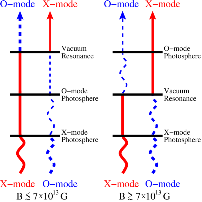
Figure 14: A schematic diagram illustrating how vacuum polarization-induced mode conversion affects the emergent radiation from a magnetized NS atmosphere. The photosphere is defined by where the optical depth (measured from the surface) is 2/3 and is where the photon decouples from the matter. The left side applies to the “normal” field regime [$B\mathrel{\raise 1.29167pt\hbox{$<$}\mkern-14.0mu\lower 2.58334pt\hbox{$\sim$}}7\times 10^{13}$ G; see Eq. (143)], in which the vacuum resonance lies outside the photospheres of the two modes. The right side applies to the “superstrong” field regime ($B\mathrel{\raise 1.29167pt\hbox{$>$}\mkern-14.0mu\lower 2.58334pt\hbox{$\sim$}}7\times 10^{13}$ G), in which the vacuum resonance lies between the two photospheres. In this diagram, complete adiabatic mode conversion is assumed across the vacuum resonance. From Ho & Lai (2004).

Vacuum polarization can dramatically affect the surface emission from magnetized NSs (Lai & Ho 2002,2003a). As discussed in §4.2-4.3, quantum electrodynamics predicts that in strong magnetic fields the vacuum becomes birefringent. In a magnetized NS atmosphere, both the plasma and vacuum polarization contribute to the dielectric property of the medium, and a “vacuum resonance” arises when these two contributions “compensate” each other. When a photon propagates outward in the NS atmosphere, it may convert from one mode into another as it traverses the vacuum resonance. Because the two photon modes have very different opacities, the vacuum polarization-induced mode conversion can significantly affect radiative transfer in magnetized atmospheres. When the vacuum polarization effect is neglected (nv), the decoupling densities of the O-mode and X-mode photons (i.e., the densities of their respective photospheres) are approximately given by (see Lai & Ho 2002)

$$\rho_{\rm O,nv} \approx 0.42\,T_{6}^{-1/4}E_{1}^{3/2}S^{-1/2}\mbox{ g cm${}^{-3}$}$$ (141)

$$\rho_{\rm X,nv} \approx 486\,T_{6}^{-1/4}E_{1}^{1/2}S^{-1/2}B_{14}\mbox{ g cm${}^{-3}$},$$ (142)

where $T_{6}=T/(10^{6}\,{\rm K})$ and $S=1-e^{-E/k_{B}T}$. Thus the X-mode photons are produced in deeper, hotter layers in the atmosphere than the O-mode photons. When vacuum polarization is taken into account, the decoupling densities can be altered depending on the location of the vacuum resonance $\rho_{V}$ relative to $\rho_{\rm O,nv}$ and $\rho_{\rm X,nv}$. For “normal” magnetic fields, $B<B_{l}$, with

$$B_{l}\approx 6.6\times 10^{13}\,T_{6}^{-1/8}E_{1}^{-1/4}S^{-1/4}\mbox{ G},$$ (143)

the vacuum resonance lies outside both photospheres ($\rho_{V}<\rho_{\rm O,nv}<\rho_{\rm X,nv}$), and the net thermal spectrum is not affected by the vacuum resonance. For superstrong magnetic fields, $B>B_{l}$, the vacuum resonance lies between these two photospheres ($\rho_{\rm O,nv}<\rho_{V}<\rho_{\rm X,nv}$), and the effective decoupling depths of the photons are changed. Indeed, we see from Fig. 14 that mode conversion makes the effective decoupling density of X-mode photons (which carry the bulk of the thermal energy) smaller, thereby depleting the high-energy tail of the spectrum and making the spectrum closer to black-body (although the spectrum is still harder than black-body because of nongrey opacities). This expectation is borne out in the atmosphere model calculations (Ho & Lai 2003). Another important effect of vacuum polarization on the spectrum is the suppression of proton cyclotron lines and other spectral lines (Ho & Lai 2003; Ho et al. 2003). The physical origin for such line suppression is related to the depletion of continuum flux, which makes the decoupling depths inside and outside the line similar. It was suggested (Ho & Lai 2003) that the absence of cyclotron lines in the quiescent spectra of several magnetars (e.g., Juett et al 2002; Patel et al. 2003) is a natural consequence of the vacuum polarization effect at work in these systems, and the detection of lines in several dim isolated neutron stars (see §8.1) is also consistent with this picture (Ho & Lai 2004).

Most studies of radiative transfer in magnetized NS atmospheres rely on solving the transfer equations for the specific intensities of the two photon modes (e.g. Meszaros 1992; Zavlin & Pavlov 2002). These equations cannot properly handle the vacuum-induced mode conversion phenomenon. This is because mode conversion intrinsically involves the interference between the modes. In particular, photons with energies 0.3-2 keV (this is the energy range in which the bulk of the radiation comes out and spectral lines are expected for $B\sim 10^{14}$ G) are only partially converted across the vacuum resonance. The other problem with the modal description of radiative transport is that it is valid only in the limit of large Faraday depolarization (Gnedin & Pavlov 1974), which is not always satisfied near the vacuum resonance, especially for superstrong magnetic fields (Lai & Ho 2003a). Also, in the presence of dissipation, the two photon modes can collapse near the resonance (see §4.3), making the modal description meaningless. To account for the vacuum resonance effect in a quantitative manner, one must solve the transfer equations in terms of the photon intensity matrix (Lai & Ho 2003a) and properly take into account of the probability of mode conversion (van Adelsberg & Lai 2006). Figure 15 depicts an example of such calculation: we see that a superstrong magnetic field indeed suppresses the high-energy tail of the thermal spectrum and reduces width of spectral lines that may be present.

Figure 15: The spectrum of a fully ionized hydrogen atmosphere with $B=5\times 10^{14}$ G and $T_{\rm eff}=5\times 10^{6}$ K. The solid line shows the result when the vacuum polarization effect is properly taken into account (including partial mode conversion at the vacuum resonance), the dotted line shows the result when the vacuum effect is turned off, and the dashed line is for a blackbody with $T=5\times 10^{6}$ K. The $E_{ci}=0.63$ keV ion cyclotron feature is prominent in the “no vacuum” curve, but is suppressed in the “partial conv” curve. From van Adelsberg & Lai (2006).

We note that even for NSs with “ordinary” field strengths ($10^{12}\mathrel{\raise 1.29167pt\hbox{$<$}\mkern-14.0mu\lower 2.58334pt\hbox{$\sim$}}B\mathrel{\raise 1.29167pt\hbox{$<$}\mkern-14.0mu\lower 2.58334pt\hbox{$\sim$}}7\times 10^{13}$ G), vacuum polarization can affect the X-ray polarization signals of the thermal emission in a significant way (Lai & Ho 2003b). In particular, the vacuum resonance effect gives rise to an unique energy-dependent polarization signature: since the mode conversion probability depends on the photon energy (§4.4), the plane of linear polarization at $E\mathrel{\raise 1.29167pt\hbox{$<$}\mkern-14.0mu\lower 2.58334pt\hbox{$\sim$}}1$ keV is perpendicular to that at $E\mathrel{\raise 1.29167pt\hbox{$>$}\mkern-14.0mu\lower 2.58334pt\hbox{$\sim$}}4$ keV. By contrast, for superstrong field strengths ($B\mathrel{\raise 1.29167pt\hbox{$>$}\mkern-14.0mu\lower 2.58334pt\hbox{$\sim$}}7\times 10^{13}$ G), the polarization planes at different energies coincide. Vacuum polarization is also important for aligning the polarization vectors of photons emitted from different patches of the NS, thus ensuring an appreciable net polarization fraction at the observer (Heyl et al. 2003; see §4.4). The detection of polarized X-rays from neutron stars can provide a direct probe of strong-field quantum electrodynamics and constrain the neutron star magnetic field and geometry.

8.4 Partially Ionized Atmospheres and Radiation from Condensed Surfaces

For sufficiently strong magnetic field and/or low temperature, bound species have non-negligible abundances in the NS atmosphere. Early considerations of partially ionized atmospheres (e.g., Rajagopal et al. 1997) relied on oversimplified treatments of atomic physics and nonideal plasma effects in strong magnetic fields. In recent years, significant progress has been made in studying partially ionized hydrogen plasmas: The binding energies and radiative transition rates, incorporating the center-of-mass motion effects (see §3.1), have been calculated for the H atom (Potekhin 1994; Potekhin & Pavlov 1997); these atomic data have been implemented in calculations of thermodynamic functions (including ionization equilibrium; see §6.4) and radiative opacities (Potekhin et al. 1999; Potekhin & Chabrier 2003,2004). The bound species contribute to the bound-bound and bound-free opacities, which, because of the center-of-mass motion effect, do not have a narrow width or sharp edge. In addition, the bound species affect the dielectric tensor of the medium and hence the polarization properties of the normal modes; these were studied by Potekhin et al. (2004) using the Kramers-Kronig relation between the real and imaginary parts of the plasma polarizability. All these physical ingredients have been incorporated into NS atmosphere models to produce the spectrum of surface emission (Ho et al. 2003; Potekhin et al. 2004). An example is shown in Fig. 16, clearly demonstrating the importance of the partial-ionization effects.

Figure 16: Spectral flux as a function of the photon energy $E$. Left panel: The case of a partially ionized hydrogen atmosphere model (solid line) at $B=10^{13}$ G (field normal to the surface) and $T_{\rm eff}=10^{6}$ K is compared with the fully ionized model (dashed line) and with the blackbody spectrum (dotted line). Adapted from Ho et al. (2003) and Potekhin et al. (2004,2006). Right panel: The cases of condensed Fe surface ($B=10^{12}$ G, short-dashed line; $10^{13}$ G, dotted line) and H surface ($B=10^{14}$ G, long-dashed line) at temperature $T=10^{6}$ K, compared with the blackbody spectrum (solid line). Adapted from van Adelsberg et al. (2005).

As discussed in §6.4, for sufficiently low temperatures and/or strong magnetic fields, the atmosphere may undergo a phase transition into a condensed state. Thermal emission from such a condensed (Fe or H) surface was studied by van Adelsberg et al. (2005) (cf. Brinkmann 1980; Turolla et al. 2004; Perez-Azorin et al. 2005). Obviously, the standard radiative transfer equation does not apply inside the condensed phase. Instead, we can apply the Kirchkoff’s law for a macroscopic object (generalized for polarized radiation; see §3.1 of van Adelsberg et al. 2005): We calculate the (polarization-averaged) reflectivity of the surface for a incident ray with incident angle $\theta$; then the emission intensity of the surface is simply $I_{\nu}=\left[1-R_{\nu}(\theta)\right]B_{\nu}(T)$, where $B_{\nu}(T)$ is the Planck function. To calculate $R_{\nu}(\theta)$, we can approximate the dielectric tensor of the condensed surface using the quasi-electron gas approximation, with and without the ion response. For a smooth condensed surface, the overall emission is reduced from the blackbody by less than a factor of 2, The spectrum exhibits modest deviation from blackbody across a wide energy range, and shows mild absorption features associated with the ion cyclotron frequency and the electron plasma frequency in the condensed matter. Examples of the spectrum for different models of the surface are shown on the right panel of Fig.  16. If the surface is rough (as is likely in the Fe case), the surface reflectivity will be close to zero, making emission spectrum even closer to blackbody. It is possible that the almost perfect blackbody spectrum in the X-ray band observed from RX J1856.5-3754 (see §8.1) is a result of such condensed surface emission, although an expanation for the excess optical emission is still called for.

8.5 Resonant Scatterings of Surface Emission

An interesting issue concerns the possibility that thermal emission from the NS surface may be modified by scatterings in the magnetospheric plasma. Since a thermal X-ray photon has energy less than the electron cyclotron energy ($E_{ce}=11.6\,B_{12}$ keV) at the stellar surface, as the photon passes through the magnetosphere, it goes through the electron cyclotron resonance ($E=E_{ce}$) where enhanced scattering occurs. For the Goldreich-Julian charge density in the closed magnetosphere, the optical depth of such scattering is negligible, thus the surface emission will not be modified (Rajagopal & Romani 1997). Ruderman (2003) suggested that a larger density of pair plasmas may be present in the magnetosphere, maintained by conversion of $\gamma$-rays from the NS’s polar-cap and/or out-gap accelerators. Partly motivated by the observational puzzles associated with the spectra of isolated NSs, he further suggested that resonant scattering of thermal photons will result in a Planck-like spectrum that is modified from the seed surface spectrum (see also Wang et al. 1998; Lyutikov & Gavriil 2006). Also, if the plasma is sufficiently hot, it can Compton upscatter the thermal photons. While this scenario may be plausible for energetic rotation-powered pulsars, the situation is not clear for the dim, radio-quiet isolated NSs, given the absence of any nonthermal emission signature from these stars. For active magnetars, a corona consisting mainly of relativistic electron-positron pairs can be generated by crustal magnetic field twisting/shearing due to starquakes, with the plasma density much higher (by a factor of order $c/\Omega r$) than the Goldreich-Julian value (Thompson et al. 2002; Thompson & Beloborodov 2005). Such a corona plasma can significantly modify the surface radiation by multiple scatterings; this may explain the $2-10$ keV soft tail of the magnetar surface emission.

9 Non-Thermal Radiation of Rotation-Powered Pulsars

There is abundant evidence that rotation-powered pulsars must be capable of particle acceleration to energies of at least 10 TeV. Pulsed $\gamma$-rays above 100 MeV have been detected from seven pulsars with high significance and about five others with less significance (Kanbach 2002). Some 60 pulsars have been detected at X-ray energies with about 30 having detectable pulsations (Kaspi et al. 2005). Both the acceleration voltage and the high-energy luminosities required can originate from the rotation of a dipole field, if the surface magnetic fields $B_{s}$ are in fact those required to produce the observed rate of spin-down by magnetic dipole torques [see Eqn (1)]. The vacuum potential drop across the open field lines is

$$V_{\rm pc}\simeq{1\over 2}\left({2\pi\over cP}\right)^{2}\,B_{s}R^{3}=6\times 10^{12}\,{\rm eV}\,P^{-2}\,B_{12},$$ (144)

where $B_{12}\equiv B_{s}/10^{12}$ G and $P$ is the pulsar spin period (in s). The fraction of this potential available for particle acceleration varies among different models and from source to source (see Harding 2005 for review), but the overall picture seems energetically self-consistent (although unsolved problems such as global current closure still exist). Two accelerator sites have been studied in most detail and two main types of model have developed. Polar cap models (Daugherty & Harding 1996, Usov & Melrose 1996) are based on particle acceleration beginning near the magnetic poles, where the magnetic fields are high and one-photon pair creation (§5.4.1) usually dominates over two-photon pair creation. Outer gap models (Cheng et al. 1986, Romani 1996) are based on acceleration in vacuum gaps in the outer magnetosphere where the magnetic fields are too low for one-photon pair creation, but pairs may be created by interactions of $\gamma$-rays produced by gap-accelerated particles with X-ray photons from either the gap or the hot neutron star.

9.1 Electromagnetic cascades

9.1.1 Polar cap cascades

The combination of high particle energies and magnetic field strength approaching, and in some sources exceeding, the critical field allow very favorable conditions for pair creation and electromagnetic cascades (Sturrock 1971) that can greatly enhance the number of particles in a pulsar magnetosphere (Daugherty & Harding 1982). The accelerated particles moving along magnetic field lines with high Lorentz factors radiate $\gamma$-ray photons at very small angles to the field ($\theta_{0}\sim 1/\gamma$), so the one-photon pair production rate for these photons is initially zero. However, as they propagate through the curved dipole field, their angle increases until the threshold condition, $\epsilon\sin\theta=2$, is reached and the attenuation coefficient becomes large. Each member of the pair will be produced in a Landau state whose maximum principal quantum number is $n_{\rm max}=2\epsilon^{\prime}(\epsilon^{\prime}-2)/B^{\prime}$ (Daugherty & Harding 1983), where $\epsilon^{\prime}=\epsilon\sin\theta$ is the photon energy in the frame in which it propagates perpendicular to the local magnetic field. From the pair production condition, $\chi\equiv\epsilon B^{\prime}\sin\theta/2\buildrel>\over{\sim}0.1$, an estimate for the maximum pair Landau state is

$$n_{\rm max}\simeq{0.4\over B^{\prime 2}}\,\left({0.2\over B^{\prime}}-2\right).$$ (145)

When the local field $B\lower 2.0pt\hbox{$\,\buildrel\scriptstyle<\over{\scriptstyle\sim}\,$}0.1B_{Q}$, pairs will be created above threshold in highly excited Landau states and the excitation level is quite sensitive to field strength, $n_{\rm max}\propto 1/B^{\prime 3}$. The pairs will decay through emission of synchrotron/cyclotron photons, many of which will produce more pairs in excited states. A pair cascade can be sustained in such a way through several generations, with pair multiplicities reaching as high as $10^{3}-10^{4}$ (pairs per primary electron) (Hibschmann & Arons 2001, Arendt & Eilek 2002). In high-field pulsars, where $B\buildrel>\over{\sim}0.1B_{Q}$ near the neutron star surface, the pair creation attenuation coefficient is high enough for pair creation near threshold, so pairs are produced in very low Landau states. In this case, cascade pair multiplicities are lower since the number of cyclotron photons drop significantly (Baring & Harding 2001). Bound pair production (cf. §5.5) also becomes important for $B\buildrel>\over{\sim}0.1B_{Q}$, which will further lower the pair multiplicity. When $B\buildrel>\over{\sim}B_{Q}$, photon splitting dominates over pair production, as was discussed in §5.6. Further reduction of the cascade pair yield in this regime then depends on whether and at what field strength additional splitting modes are possible. If all three modes permitted by QED are operating, then a full photon splitting cascade replaces the pair cascade and a complete suppression of pairs occurs (Baring & Harding 2001). If only the $\perp\rightarrow\parallel\parallel$ mode permitted in the non-dispersive limit is operating, as is more likely, then no suppression of pair yields occurs by photon splitting alone. However, the $\parallel$ mode photons will create bound rather than free pairs in a strong field (Shabad & Usov 1985, 1986), which at least delays the creation of real pairs until the bound pair is dissociated by radiation and/or electric fields (Usov & Melrose 1996) or moves to higher altitude where the field is smaller. The pair cascade may then resume, but changes to pair yields in this case have not been studied. The screening (see next paragraph) of the electric field is also delayed by splitting and creation of bound pairs, effectively increasing the accelerating potential. The effect of bound pair creation on polar cap acceleration has been studied by Usov & Melrose (1996).

In the case of young pulsars with high surface fields, the pair cascades are limited by screening of the electric field by the pairs as they accelerate in opposite directions (Arons & Scharlemann 1979). Such pulsars are capable of accelerating primary particles to high enough energies ($\gamma\sim 10^{7}$) that their curvature radiation photons can create pairs to initiate the cascade. The curvature-radiation initiated cascades produce high multiplicities over a small fraction of a neutron star radius and can screen the $E_{\parallel}$ on that length scale (Harding & Muslimov 2001). Older pulsars with lower magnetic fields have difficulty accelerating particles fast enough for their curvature photons to pair produce before the magnetic field drops. In this case, inverse-Compton (ICS) photons that are produced by the particles at a lower energy ($\gamma\sim 10^{4}-10^{6}$), scattering thermal X-rays from the neutron star surface, can create pairs at lower altitude (Zhang & Qiao 1996). However, the ICS-initiated cascades have much lower multiplicity, since the emission rate decreases as the particles’ energy increases (in constrast to the CR emission rate which increases as with energy), and are not robust enough to screen the $E_{\parallel}$ (Harding & Muslimov 2002). These cascades are thus limited by the increasing energy of the accelerating particles and the $E_{\parallel}$ ultimately saturates at several polar cap radii by geometric effects. In the case of millisecond pulsars having extremely low magnetic fields, but very short periods, two-photon pair creation through interaction of curvature radiation or ICS photons with thermal X-ray photons from the neutron star surface can dominate over one-photon pair creation (Zhang & Qiao 1998, Harding et al. 2002). Ultimately, as the pulsar ages the polar cap potential drop becomes too low to produce pairs of any kind (Harding & Mulsimov 2002, Harding et al. 2002). The resulting “death line” in $P$-$\dot{P}$ space accounts for the abrupt decrease in numbers of radio pulsars at periods longer than a few seconds (see Figure 1).

9.1.2 Outer gap cascades

Pair cascades in the outer magnetosphere of a pulsar, where magnetic field strengths are in the range $B\sim 10^{5}-10^{9}$ G, must be sustained by two-photon pair creation. The cascade-initiating particles are accelerated to high Lorentz factors in near-vacuum electric fields that develop as a result of the depletion of charge beyond the null-charge surface $\Omega\cdot B=0$ (Cheng, Ho & Ruderman 1986). They radiate curvature, or more accurately, synchro-curvature (Zhang & Cheng 1996) $\gamma$ rays tangent to magnetic field lines within the gap and propagate until they interact with soft photons, either from the hot neutron star surface or from lower energy gap radiation, to create a pairs. The pair accelerates in opposite directions, emitting more synchro-curvature radiation photons which produce more pairs and the secondary particles supply current through the gap. The multiplicity of outer-gap cascades could be quite high (Hirotani, priv. comm. 2005), with most of the pairs produced by collisions between downward-going gamma-rays and surface X-rays, with magnetic pair creation being important near the neutron star surface. These cascades are limited by screening of the $E_{\parallel}$ in directions both parallel and perpendicular to the magnetic field (Cheng et al. 2000, Hirotani & Shibata 2001), taking into account the curvature of the field lines. The gaps can also be self-limited if the thermal X rays supplied by the hot neutron star surface require heating by gap-accelerated particles flowing downward (Cheng 1994, Zhang & Cheng 1997). However, neutron star cooling that releases the latent heat of formation, provides most of the surface X rays in the youngest pulsars.

Older pulsars cannot sustain pair cascades in an outer gap, because the $E_{\parallel}$ is smaller and even the potential drop across the entire outer magnetosphere is not sufficient for pair creation. An outer-gap death line in $P$-$\dot{P}$ space is thus predicted (Chen & Ruderman 1993), which may also be a function of pulsar inclination angle (Zhang et al. 2004), and suggests that pulsars older than $\tau\sim 10^{7}$ yr do not have outer gaps or the associated high-energy emission.

9.2 Observable signatures of high-field physics

There are several predicted features of non-thermal pulsar emission that would be signatures of physical processes operating exclusively in magnetic fields near $B_{Q}$. The spectra of polar cap cascade emission will display high-energy cutoffs due to one-photon pair creation attenuation (Daugherty & Harding 1982). Such cutoffs are distinguishable by their very sharp, super-exponential shape, so that the observed spectra will have the form

$$f(\epsilon)=A\epsilon^{-a}\,\exp\left[{-C_{1\gamma}\exp\left(-{\epsilon^{1\gamma}_{\rm esc}/\epsilon}\right)}\right]$$ (146)

where $a$ is the power-law index, $C_{1\gamma}=0.2(\alpha/\lambda\hbox to0.0pt{\hss--})(B^{\prime}R^{2}/\rho)$ and $\epsilon_{\rm esc}$ is the escape energy from the magnetosphere for photons of energy $\epsilon$ (Harding et al. 1997, Harding 2001),

$$\epsilon^{1\gamma}_{\rm esc}\sim 2\,\,{\rm GeV}\,P^{1/2}\,\left({r_{0}\over R}\right)^{1/2}\,{\rm max}\left\{0.1,\,B_{s,12}^{-1}\,\left({r_{0}\over R}\right)^{3}\right\}$$ (147)

or the energy above which photons emitted from a radius $r_{0}$ can escape the magnetosphere without pair attenuation. The above estimate of the escape energy assumes that the condition for pair attenuation is $\chi\sim 0.2$ for $B^{\prime}\lower 2.0pt\hbox{$\,\buildrel\scriptstyle<\over{\scriptstyle\sim}\,$}0.1$ and $\epsilon\sin\theta=2$, the threshold condition, for $B^{\prime}\buildrel>\over{\sim}0.1$, that $\sin\theta\sim R/\rho$, where $\rho$ is the field line radius of curvature at the polar cap rim and that $\rho$ and $B^{\prime}$ are evaluated at the photon emission radius $r$. The cutoff in the spectrum of polar cap cascades that are extended over more than a stellar radius will be somewhat more gradual than Eqn (146) due to variations in both the field strength and radius of curvature. Nevertheless, the cutoff should still be distinguishable from a simple exponentional.

For pulsars with high magnetic fields $B^{\prime}\buildrel>\over{\sim}1$, photon splitting dominates the attenuation of polar cap cascade photons in the $\perp$ mode (see §5.6), while $\parallel$ mode photons are attenuated by pair production. The photon splitting cutoff occurs at roughly the escape energy for photon splitting,

$$\epsilon^{sp}_{esc}\sim 93\,{\rm MeV}\,\,P^{3/5}\,\left({r_{0}\over R}\right)^{3/5}\,\left\{\begin{array}[]{lr}B^{\prime-6/5},&B^{\prime}\lower 2.0pt\hbox{$\,\buildrel\scriptstyle<\over{\scriptstyle\sim}\,$}1\\ 1,&B^{\prime}\buildrel>\over{\sim}1\\ \end{array}\right.$$ (148)

where $B^{\prime}=(r_{0}/R)^{-3}$ is the local field strength. At high fields the photon splitting escape energy will be lower than that for pair production. The photon splitting cutoff will also have a more gradual shape since the attenuation coefficient is power law rather than exponential. Because the $\perp$ mode photons are attenuated at a lower energy than the $\parallel$ mode photons, the spectrum will be 100% polarized in the $\parallel$ mode in the energy band between $\epsilon^{sp}_{esc}$ and $\epsilon^{1\gamma}_{esc}$ (Harding et al. 1997). This band will grow as the field strength increases, as the $\epsilon^{sp}_{esc}$ decreases and the field dependence of $\epsilon^{1\gamma}_{esc}$ saturates for $B^{\prime}\buildrel>\over{\sim}1$. If such strong polarization in $\gamma$-ray pulsar spectra near the high energy cutoff is detected by future X-ray and $\gamma$-ray polarimeters, it would be a clear signature of photon splitting.

The above estimates for pair creation and photon splitting escape energies assumes flat spacetime. Near a neutron star, depending on its compactness (i.e. equation of state), general relativistic effects including photon red-shift, light bending and changes to the dipole field are important for photon attenuation (Gonthier & Harding 1994). For standard neutron star compactness, curved spacetime effects will lower the escape energies for both pair creation and photon splitting by a factor of about 2 (Harding et al. 1997, Baring & Harding 2001).

10 Radiation of Magnetars

SGRs and AXPs were both discovered several decades ago, but they have only recently been recognized as similar objects (for detailed review, see Woods & Thompson 2005, Heyl 2005). SGRs were first detected around 1979 as $\gamma$-ray transients and were thought to be a type of classical $\gamma$-ray burst. They undergo repeated bursts with several tenths of second duration and average energy $10^{40}-10^{41}\,\rm erg$, and their bursting often occurs in episodes spaced years apart. They more rarely undergo giant superflares of total energy $10^{45}-10^{47}\,\rm erg$, consisting of an initial spike of duration several hundred ms followed by a longer decay of duration several hundred seconds showing pulsations. Such superflares have been observed in three SGR sources, SGR0526-66 (the famous 5th March 1979 event), SGR1900+14 (Hurley et al. 1999) and very recently in SGR1806-20 (Hurley et al. 2005; Palmer et al. 2005). In 1998, SGR1806-20 was discovered to have 7.47 s pulsations in its quiescent X-ray emission (Kouveliotou et al. 1998) (and a large $\dot{P}$ that implied a huge surface magnetic field of $\simeq 10^{15}$ G if due to dipole spin-down. Quiescent periodicities of 8 s and 5.16 s and large $\dot{P}$ were subsequently detected in SGR0526-66 and SGR1900+14, implying similarly high surface magnetic fields. In all three sources, the quiescent periods are the same periods seen in the decay phases of their superflares. The quiescent pulse profiles are very broad and undergo dramatic changes just before and after superflares. The profiles are often more complex, with multiple peaks before flares, changing to more simple single peaks profiles following the flares. All of the SGRs lie near the Galactic plane and are thought to have distances around 10-15 kpc (except for SGR0526-66, which is in the LMC).

The quiescent spectra of AXPs and SGRs consist of a thermal component fit by $\sim$ 0.5-1 keV blackbodies and one or more non-thermal components, with X-ray luminosity $10^{35}-10^{36}$ erg s^-1. Until recently, the non-thermal spectra below 10 keV were fit with steep power laws having indices $\Gamma\sim 2-4$ (spectral flux $\propto\epsilon^{-\Gamma}$). When INTEGRAL and RXTE recently measured the spectra above 10 keV for the first time hard, non-thermal components were discovered in three AXPs, and also SGR 1806-20. In two of the AXPs, the differential spectra between 10 keV and 50 keV are extremely flat: 1E 1841-045 (Kuiper et al. 2004) has a power-law index of $s=0.94$ and 4U 0142+61 (Hartog et al. 2004) displays an index of $s=0.45$, both much flatter than the steep non-thermal components in the classic X-ray band. RXS J1708-40 possesses a slightly steeper continuum with $s=1.18$. The non-thermal tail of quiescent emission in SGR 1806-20 is similarly pronounced (Mereghetti et al. 2005, Molkov et al. 2005)), but somewhat steeper, with an index of $s=1.6-1.9$ extending beyond 100 keV. The luminosity in hard x-rays ($\sim 100$ keV), $\sim 10^{36}$ erg s^-1, even exceeds the thermal luminosity from the stellar surface. Such hard non-thermal components require continuous particle acceleration during the quiescent state.

Although it was proposed early on (Ramaty et al. 1980, Katz 1982) that SGRs were neutron stars with strong magnetic fields in the range $B_{S}\sim 10^{11}-10^{13}$ G to confine the burst radiation, it was sometime later that surface magnetic fields exceeding $10^{14}$ G were actually predicted for these objects (Duncan & Thompson 1992; Thompson & Duncan 1995,1996). Duncan & Thompson (DT), exploring the origin of neutron star magnetic fields, conjectured that in dynamo models magnetic fields $3\times 10^{17}\,{\rm G}\,(P_{i}/1\,\rm ms)^{-1}$ could be generated in nascent neutron stars with initial periods $P_{i}$ in the ms range (see Thompson & Duncan 1993 and §7.2). Paczynski (1992) deduced that SGR0526-66 must have a magnetic field of $5\times 10^{14}$ G to lower the magnetic scattering cross section (§5.3), and therefore raise the Eddington Limit to the luminosity of the repeating bursts at a distance of the LMC (see also Miller 1995). This is coincidentally the field required if its spin-down age at rotation period of 8 s is compatible with the age of its associated supernova remnant N49 (Duncan & Thompson 1992). Fields of this magnitude will decay of much shorter timescales due to the onset of ambipolar diffusion (§7)

$$t_{\rm Amb}\cong 10^{4}yr\left({\frac{{B_{core}}}{{10^{15}G}}}\right)^{-2}.$$ (149)

Diffusion of magnetic flux out of the NS core on these timescales provides the power to magnetars in the DT model. Magnetar-strength fields also apply higher stresses to the stellar crust, so that the yield strain can exceed the crustal strength. This property is responsible for the small SGR and AXP bursts in the DT model (Thompson & Duncan 1996). If a toroidal component of the field $B_{core}>10^{15}$ G develops in the interior of the star, it can twist the external field (Thompson & Duncan 2001). Such action can cause the superflares if the twisted field lines reconnect. The field line twists following starquakes (and the associated X-ray burst activities) may last for years and lead to significant heating of the near vicinity of the star (Thompson et al. 2002; Thompson & Beloborodov 2005). Finally, due to the much faster heat transport in very strong magnetic fields, there is a modest increase in the heat flux through the crust (§6.3; Heyl & Kulkarni 1998, see Figure 17). All these effects may explain the much hotter surface temperatures of magnetars and the high quiescent X-ray emission.

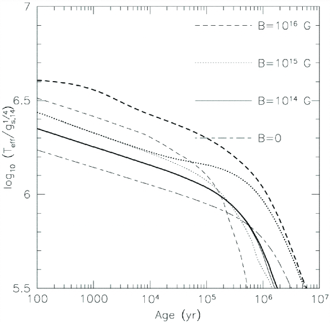
Figure 17: Evolution of effective neutron star surface temperature when the magnetic field decays through the irrotational mode, for different initial magnetic fields. The light lines are results for no field decay and the long-short dashed line shows the cooling evolution for an unmagnetized neutron star. From Heyl & Kulkarni (1998).

The magnetar model has had success in accounting for the energetics of the burst and quiescent emission in terms of the response of the neutron star to the enormous stresses of field decay. According to the DT model (Thompson & Duncan 1995), the magnetar superflares results from reconnection of sheared or twisted external field lines, leading to particle acceleration and radiation of hard emission (see also Lyutikov 2006). The estimated total energy of such events,

$$\frac{{B_{core}^{2}}}{{8\pi}}R^{3}\approx 4\times 10^{46}{\rm erg}\left({\frac{{B_{core}}}{{10^{15}G}}}\right)^{2},$$ (150)

is similar to observed luminosities of superflares. The smaller bursts result from cracking of the crust, which is continually overstressed by diffusion of magnetic flux from the NS interior. The shaking of magnetic footpoints then excites Alfven waves that accelerate particles. The energy radiated in such events would be

$$E_{SGR}\cong 10^{41}{\rm erg}\left({\frac{{B_{S}}}{{10^{15}G}}}\right)^{-2}\left({\frac{l}{{\rm 1km}}}\right)^{2}\left({\frac{{\theta_{\max}}}{{10^{-3}}}}\right)^{2},$$ (151)

where $l$ is the length scale of the displacements, $B_{S}$ is the crustal field and $\theta_{\max}$ is the yield strain of the crust. The quiescent emission in the DT model is power by magnetic field decay through conduction of heat from the core. The NS crust is heated to a temperature of

$$T_{crust}\cong 1.3\times 10^{6}K\left({\frac{{T_{core}}}{{10^{8}K}}}\right)^{5/9}$$ (152)

where $T_{core}$ is the core temperature, and luminosity

$$L_{\rm{x}}\cong 6\times 10^{35}{\rm ergs^{-1}}\left({\frac{{B_{core}}}{{10^{16}G}}}\right)^{4.4}.$$ (153)

Model atmospheres for the quiescent thermal emission from magnetars was discussed in §8.

Magnetar models have so far not had complete success in accounting for the spectrum of the burst radiation. In the DT model, $\gamma$ rays are produced by scattering of X-rays from the neutron star surface by particles accelerated after the energy released in crust cracking. In the equatorial region, the $\gamma$ rays are attenuated by photon splitting and pair creation (assuming that only the $\perp\rightarrow\parallel\parallel$ splitting mode operates), forming a pair plasma that is optically thick to Compton scattering at an equilibrium temperature of $\sim 100$ keV (Thompson & Duncan 1995) and confined by the magnetic field. Such an estimate results from the deposition of an energy $\sim 10^{41}$ erg into a volume $\sim R_{\rm max}^{3}$, with $R_{\rm max}\sim 10\,R$. Since the observed burst spectra are fitted with much lower temperatures ($\sim 10-20$ keV), we cannot be viewing the pair plasma directly, and perhaps the final spectrum is formed at small optical depths. Thompson & Duncan (1995) argue that if thermal equilibrium of the pair plasma is maintained by photon splitting balancing photon merging (its inverse process), then the photon number is increased while the temperature decreases to $T_{\rm sp}\sim 11\,{\rm keV}$, which represents a lower limit on the temperature of the emergent SGR burst spectra. But this is a crude estimate of the actual temperature of the observed thermal spectrum since scattering and further splitting can occur outside the splitting photosphere, the radius at which $B\sim B_{Q}$. The radiative transfer and spectrum of this hot, highly magnetized, and probably dynamic, pair plasma has not been fully modeled. Baring (1995, Harding & Baring 1996) modeled spectra resulting from photon splitting cascades assuming that the three splitting modes allowed by QED (see §5.6) operate at magnetar field strengths. The splitting cascade spectra are quasi-Maxwellian in shape and the spectral peak saturates in fields above $\sim 5-10B_{Q}$ at around 20-30 keV due to the saturation of the photon splitting rate in high fields. Although this model could explain the magnetar burst spectral shape, it has not been shown that both photon polarization modes can split in magnetar fields.

Heyl & Hernquist (2005a) propose an alternative model of magnetar radiation that appeals to the non-linearity of electrodynamics due to vacuum polarization in a strong magnetic field. This model assumes that the power is generated by crustal fractures or field re-arrangement, as in the DT model, but postulates that the energy is transported primarily by magnetohydrodynamic fast-mode waves rather than by Alfven waves. The details of the generation of these waves, whether they are produced directly or through interaction of Alfven waves, is not addressed. The fast MHD waves that travel away from the neutron star surface with sufficiently large amplitude and short wavelength can break down into electron-positron pairs (Heyl & Hernquist 1999) if they form discontinuities in the magnetized vacuum on the order of a Compton wavelength. The bulk of the pairs form a hot, optically-thick fireball, similar to that produced in the DT model. Unfortunately, if the burst spectrum is produced by such an optically-thick pair fireball, the actual mechanisms by which it formed are erased and will not be detectable from observation.

Several models have been suggested for explaining the hard component recently discovered in quiescent emission. Baring (2004) proposes that resonant Compton upscattering of thermal X-rays by accelerated particles in open field region produces the quiescent hard emission. Thompson & Beloborodov (2005) have proposed that the hard, non-thermal quiescent component is due to the creation of a strong $E_{\parallel}$ induced by twisting of field in closed region; this leads to synchrotron radiation from electron acceleration at high altitude, or free-free emission from a hot ($\sim 100$ keV) transition layer between the atmosphere and corona (Thompson & Beloborodov 2005). In the model of Heyl & Hernquist (2005b), a small fraction of the energy generated by the fast MHD wave breakdown goes into a non-thermal pair component which produces the hard quiescent component via a pair-synchrotron cascade.

10.1 Radio emission and pair suppression in magnetars

Although transient radio emission has been detected following superflares of SGR1900+14 (Frail et al. 1999) and SGR1806-20 (Gaensler et al. 2005), as well as the outburst of AXP XTE J1810-197 (Halpern et al. 2005), no persistent, pulsed radio emission has been detected from any SGRs or AXPs. The report of radio pulsations from SGR1900+14 (Shitov et al. 2000) was unconfirmed (Lorimer & Xilouris 2000) and probably confused with emission from the nearby radio pulsar PSR J1907+0918. It was only very recently that radio pulsations were detected from one transient AXP, XTE J1810-197 (Camilo et al. 2006), after its 2003 X-ray outburst. The fact that so few magnetars have detected radio pulsations is somewhat of a mystery given the dense pair plasmas invoked by magnetar models. It is widely believed that the bright, coherent radio emission seen from rotation-powered pulsars is produced by plasma instabilities requiring pair plasmas. One must conclude that the pair plasma instabilities operating to produce radio emission in rotation-powered pulsars are not effective in magnetar fields, that the radio emission is absorbed, or that magnetars do not produce dense pair plasmas. The first option is complicated by the fact that radio pulsars with magnetar fields exist, so that the inability of pairs to generate the coherent radio emission in magnetars must be disrupted by the higher energy densities in their magnetospheres. During magnetar bursts, the plasma frequency is almost surely above radio frequencies if even a small fraction of the total energy density resides in pairs, so that any radio emission would be absorbed. However, in quiescence the particle density is expected to be closer to that of the Goldreich-Julian charge of radio pulsars, which gives plasma frequencies of 1 - 10 GHz near the surface and falls of $r^{-3/2}$ above the surface. Even if the particle densities are several hundred times the Goldreich-Julian density, radio emission would only be absorbed near the stellar surface. Another reason which has been given for the absence of radio pulses is that their small polar caps predict very small radio beams that are hard to detect (Thompson & Duncan 1996). But as the number of known magnetars increases, we would expect to be in view of a few of the radio beams, and a number of radio pulsars with similarly small predicted radio beams have been discovered.

The suppression of pair creation is also a possible explanation for the absence of radio emission in magnetars. It was noted that the field strength $B\sim B_{Q}$ at which photon splitting begins to dominate the attenuation of photons near pulsar polar caps occurs at around the dividing line between radio pulsars and magnetars (Baring & Harding 1998) and would impose a death line for pair creation at high fields. However, the complete suppression of pair creation requires that both photon polarization modes undergo splitting (Baring & Harding 2001), but only the $\perp$ mode splitting is allowed under Adler’s (1971) kinematic selection rules (§5.6). Usov (2002) suggested that pair suppression could still occur if bound pair creation were also taken into account. Photons in the $\parallel$ mode will create bound pairs with both particles in the ground state, which are stable against annihilation (§5.5). Photons in the $\perp$ mode would create bound pairs with one or more particles in an excited state, which can be dissociated by ionization in spin-flip transitions, but these photons would split before creating the unstable bound pairs.

11 Accreting X-ray Pulsars

X-ray pulsars are believed to be strongly-magnetized accreting neutron stars powered by kinetic energy of infalling matter from a companion star. The magnetic fields of $10^{11}-10^{13}$ G are inferred from the pulsations that require anisotropic infall and radiation, the cyclotron lines observed in a number of pulsar spectra (Nagase 1989, dal Fiume et al. 2000), and the observed changes in pulse period (Ghosh & Lamb 1979, Bildsten et al. 1997). We can get a fairly good estimate of the effective temperature observed in X-ray pulsars from $T_{\rm eff}\simeq(L_{x}/\sigma A_{\rm cap})^{1/4}\simeq 10$ keV, where $L_{x}$ is the X-ray luminosity and $A_{\rm cap}$ is the heated polar cap area. But clearly, since pulsar spectra are not blackbody, we must have an accurate description of the radiating plasma in order to model the emission.

The conditions in the emission region are closely tied to the dynamics of the accretion flow and infall, and there are two major regimes that depend upon whether or not the radiation pressure of the emitting plasma is capable of decelerating the accretion flow. The critical luminosity $L_{\rm crit}$ where this division occurs is not accurately determined but can be estimated by requiring that the outgoing radiation pressure balance the ram pressure of the infalling matter:

$$L_{\rm crit}={GMm_{p}c\over\sigma_{\parallel}}{A_{\rm cap}\over R^{2}}\simeq 10^{36}\,\rm ergs^{-1},$$ (154)

when $\sigma_{\parallel}\sim\sigma_{T}$ and $A_{cap}=0.1R^{2}$, where $\sigma_{\parallel}$ is the magnetic Thomson scattering cross section parallel to the field, averaged over the spectrum, polarization and angles of the radiation. The value of $L_{\rm crit}$ is about one hundredth of the Eddington limit for spherical accretion, and is model dependent since the averaged cross section should include the radiation produced throughout the atmosphere in a self-consistent model. The high luminosity X-ray pulsars where $L_{x}>L_{\rm crit}$ may radiate several orders of magnitude above $L_{\rm crit}$ and even above the spherical Eddington limit. In low-luminosity sources where $L_{x}\ll L_{\rm crit}$, radiation pressure is not important in decelerating the accretion flow, in which case it may be decelerated by a collisionless shock above the neutron star surface or by Coulomb and nuclear collisions with atmospheric plasma near the surface. Most (about two thirds) of the observed X-ray pulsars fall into the high-luminosity category.

The most important effect of the neutron star magnetic field on the processes that decelerate the accretion flow and that produce the observed radiation is the quantization of particle momentum perpendicular to the field (see §2). In sources where $L_{x}\ll L_{\rm crit}$, accretion flow can convert its kinetic energy to heat either at a collisionless shock front (Basko & Sunyaev 1976) or by Coulomb collisions with thermal electrons and protons in the atmosphere (Basko & Sunyaev 1975, Pavlov & Yakovlev 1976). Self-consistent models of Coulomb-decelerated acceleration (Harding et al. 1984, Miller et al. 1989) result in thin slab-like atmospheres, since Coulomb stopping lengths are only $\sim 50\,\rm g\,cm^{-2}$ (Kirk & Galloway 1981, Pakey 1990). Models for sources with $L_{x}>L_{\rm crit}$, where radiation pressure dominates the deceleration, must solve the coupled radiation-hydrodynamic flow to find the structure of the atmosphere. In such models, a radiative shock stands off several stellar radii above the neutron star surface and the atmosphere has more of a cylindrical geometry, as radiation escapes from the sides of a decelerating mound of gas below the shock (Langer & Rappaport 1982, Kirk 1985).

The dominant cooling process in X-ray pulsar atmospheres is resonant Bremsstrahlung (or cyclotron cooling), in which an electron in the ground state is collisionally excited and deexcites through spontaneous emission, producing a cyclotron photon. The inverse process of resonant free-free absorption, where an electron is excited by absorption of a cyclotron photon and collisionally deexcited, can in some cases provide significant heating to the atmosphere. So while the vast majority of electron excitation-deexcitation events are resonant Compton scattering at the cyclotron energy the collisions, although less frequent, control the net production and destruction of cyclotron photons in these atmospheres. Another important heating and cooling process is Compton scattering, which is resonant at the cyclotron harmonics in a magnetic field. While scattering does not produce nearly as much heating and cooling as Bremsstrahlung since it does not create and destroy cyclotron photons, it exchanges energy between photons and electrons in the atmosphere (Meszaros & Ventura 1979). The presence of a strong magnetic field introduces substantial changes in the stopping length due to Coulomb scattering. A accreting proton moving along the magnetic field experiences a much smaller drag force than in the non-magnetic case because the electrons are limited to momentum transfers along the field unless they can be excited to higher states. The infalling protons must diffuse in momentum space through many small-angle collisions, gradually veering away from the magnetic field direction where their drag force will increase and they can decelerate faster. As a result, the stopping lengths are very dependent on the proton momentum diffusion and significantly larger than in an un-magnetized plasma (see, e.g., Nelson, Salpeter & Wasserman 1993).

11.1 Cyclotron lines

The cyclotron lines seen in the spectra of accreting X-ray pulsars are formed by resonant scattering (§5.3) of photons with electrons that occupy discrete Landau states. If the plasma temperature is less than $T_{B}=\epsilon_{B}/k$, then the electrons occupy primarily the ground Landau state [regime (i) of §6] and have a one-dimensional thermal distribution of momenta along the magnetic field. At magnetic field strengths typical of neutron stars, the cyclotron decay rates from excited Landau states ($n>0$), $\Gamma_{n}=4\times 10^{15}nB_{12}^{2}\,\rm s^{-1}$, are much greater than the rate of collisional excitation. Unless there are other processes that can populate the excited states on faster timescales, the bulk of the electrons are expected to occupy the ground state in a one-dimensional distribution. Under these conditions, absorption of a cyclotron photon is always followed by the emission of another photon, so resonant scattering is more important than absorption. As discussed in §5.3 , the Compton scattering cross section has sharp maxima at the cyclotron resonance (Eqn [74]) and its harmonics, so that photons scatter preferentially at these energies. Since the scattering cross section has a strong dependence on angle to the magnetic field, the cyclotron resonance scattering features (CRSFs) provide excellent diagnostics of the emission geometry as well the physical conditions (temperature and density) of the radiating plasma.

The formation of CRSFs at the fundamental and at the harmonics proceeds by very different routes. When a photon at the fundamental resonance frequency (Eqn [74] with $N=1$) scatters with an electron in the ground state the scattered photon also appears at the fundamental. The scattered photon may have a different angle, but unless the continuum photons are beamed, resonant photons from other angles scatter into view. Absorption-like features can only form in the fundamental by repeated scattering, causing diffusion of photons in energy and angle through the combined effects of electron recoil and the natural line width of the resonance (Wasserman & Salpeter 1980, Wang et al. 1989). Resonant photons can then diffuse from the line core into the line wings where the cross section drops to near $\sigma_{T}$ and they can then escape, primarily in the red wing. When a photon at the first harmonic ($N=2$) scatters with an electron from the same distribution, the scattered photon will appear most of the time at the fundamental in fields $B^{\prime}\lower 2.0pt\hbox{$\,\buildrel\scriptstyle<\over{\scriptstyle\sim}\,$}0.2$, exciting the electron to the $n=1$ state. The electron then decays through cyclotron emission, spawning an additional photon at the fundamental. Although this is technically still a resonant scattering ($n=0\rightarrow 2\rightarrow 1$ followed by $n=1\rightarrow 0$), analogous to Raman scattering in atomic physics, incident photons are destroyed in the first harmonic and the line formation here is well approximated by absorption (Fenimore et al. 1988, Wang et al. 1988, Harding & Daugherty 1991). Thus, the second and higher harmonics are formed in a similar way, with photons in the $N$th resonance exciting the electron from the ground state to the $n-1$ state, with the subsequent spawning of $n-1$ additional photons at the fundamental through single harmonic number transitions. Photon spawning partially fills in the fundamental (Wang et al. 1988), so that the line features at the cyclotron fundamental and higher harmonics will not appear in the same ratios in the observed spectrum as they do in the cross section. In magnetic fields $B^{\prime}\buildrel>\over{\sim}0.2$, the dominance of cyclotron decays to the ground state (§5.2) reduce the rate of photon spawning in the fundamental (Araya & Harding 1999) since scattering in the $N$th harmonic is more likely to produce a scattered photon in the $N$th resonance ($n=0\rightarrow N\rightarrow 0$). Formation of the harmonics in these high fields therefore proceeds more by diffusion out of the line core, as the fundamental is formed, rather than by excitation of the electron.

As in most line-formation scenarios, the broadening of the CRSFs results from a combination of natural line width, which gives a Lorentzian profile, and the Doppler effect, which gives a Gaussian profile. Due the one-dimensional momentum distribution of the electrons, the line broadening is asymmetric and dependent on viewing angle to the magnetic field, $\theta$. First order (non-relativistic) Doppler broadening alone gives a line width that is approximately

$$\Delta\epsilon_{D}\approx\epsilon_{N}(2T)^{1/2}\cos\theta,$$ (155)

where $T$ is the plasma temperature in units of $mc^{2}$ and $\epsilon_{N}$ is the resonant energy (Eqn [74]). At small viewing angles, the lines are broadened by the full Doppler motion, while in the limit of large viewing angles, only transverse (second-order) Doppler broadening contributes to the line width. Since the transverse Doppler broadening is a red shift (from time dilation), the line profiles become increasingly asymmetric at large incidence angles. The natural line width, due to the finite lifetime of excited Landau states, is approximately equal to the cyclotron decay rate from state $N$ which, in the non-relativistic limit, is

$$\Delta\epsilon_{N}\approx{4\over 3}\alpha B^{\prime 2}N$$ (156)

At large angles, $\Delta\epsilon_{N}$ provides the main contribution to the broadening on the blue side of the line. In a relativistic treatment of line broadening, the cyclotron decay rate is dependent on the electron spin, with the rates of spin-flip transitions being smaller (Herold et al. 1982).

Figure 18: Relativistic cyclotron scattering line profiles for $B^{\prime}$ = 0.24 and thermal electron temperature of 31 keV, for different viewing angles, $\mu=\cos\theta$.

Techniques for modeling CRSFs in XRP atmospheres have included either solving the equations of radiative transfer using a Feautrier method (Meszaros & Nagel 1985, Nagel 1981, Alexander & Meszaros 1991b, Burnard et al. 1988) or Monte Carlo simulation (Wang et al. 1988, Araya & Harding 1999, 2000). Given the complexities of the line transfer, these models usually assume a static atmosphere and simplified geometries, in particular homogeneous slabs, with the magnetic field perpendicular to the slab normal, or cylinders parallel to the field. An exception is the work of Arons et al. (1987) and Burnard et al. (1988) who treat a time-dependent accretion column. Such studies have generally confirmed that the shape and relative depths of the fundamental and higher harmonics of CRSF are very dependent on viewing geometry as well as geometry of the scattering plasma. In particular, CRSFs seen at small angles to the magnetic field tend to be broader with weak harmonics, whereas CRSFs seen at large angles are narrower, more asymmetric and have stronger features at higher harmonics. In slab geometry the depth of the fundamental is largest at large angles to the field, where the optical depth is largest, but in cylinder geometry the fundamental feature is largest at small angles (Araya & Harding 1999). In many cases the fundamental is flanked by emission wings, from photons escaping the line core, and may even appear completely in emission, at large angles in cylinder geometry, due to photons diffusing from smaller angles.

Given the sensitive dependence of CRSF characteristics with angle to the field, one would expect a great deal of variation in the features with rotational phase of the neutron star. This is in fact what is observed in phase resolved spectra of accreting XRPs (Heindl et al. 2004, Orlandini & dal Fiume 2001). The line depths as well as their energies change with phase, but the harmonic relationships are preserved, as would be expected of CRSFs.

12 Conclusion

In this article we have reviewed the physics that applies in extremely strong magnetic fields, the properties of strongly magnetized neutron stars, atmospheres and magnetospheres, and the present status of our understanding and models of the astrophysical sources that are their manifestation. While the use of non-relativistic quantum mechanics is adequate (even for $B>B_{Q}$) for describing bound states or any processes where the electron stays in the ground Landau level, one must use relativistic quantum mechanics (QED) in computing the rates and cross sections for many free particle and photon processes. Nearly all of the cross sections for the first and second-order free particle processes in strong magnetic fields, such as cyclotron radiation and absorption, one photon and two-photon pair creation and annihilation and Compton scattering, have been calculated and studied. Only a few of the higher-order processes, such as Bremsstrahlung and photon splitting, have been investigated since they become increasingly complex. The unusual and interesting properties of photon propagation in strong magnetic fields has been a topic of intensive study in recent years, especially after the discovery of magnetars. Among all the processes that have been investigated, vacuum polarization has been found to be of particular importance.

A variety of astrophysical sources, that include rotation-powered and accretion-powered neutron stars and the magnetars, SGRs and AXPs, are believed to be very strongly magnetized neutron stars. The processes that operate only in such strong fields may be fundamental to the functioning of these sources. For rotation-powered pulsars, one-photon pair creation is thought to be the primary process attenuating high-energy photons, and the created pairs may be critical in the production of the observed radio pulsations. We do not yet fully understand though how and why the radio emission seems to turn off well before the pulsar spin-down has ceased. Theoretical models show that pair production decreases as the pulsar ages, but does it turn off suddenly, or are there some threshold properties (e.g. multiplicity or energy spectrum) for radio emission? In the case of the magnetars, power levels far exceeding their spin-down power requires fast magnetic field decay on timescales only possible through processes such as ambipolar diffusion, that become effective in fields above $10^{14}$ G. We do not yet understand, however, why these sources are radio quiet. Is pair production suppressed by the strong field or are the collective plasma processes disrupted? Theoretical studies have so far not been able to find a convincing mechanism for the suppression of the radio emission in magnetars. Even more puzzling is the growing number of magnetars and radio pulsars having very similar spin properties, and therefore similar implied surface magnetic field strengths. Aside from their radio emission properties, radio pulsars and magnetars also have very different X-ray emission levels, transient emission and glitching behavior. What are the hidden characteristics of these sources that distinguish them? Also of interest are the emerging population of “dim” isolated neutron stars with apparently pure thermal emission. The spectral features detected in some of these sources are exciting, but their identifications remain unclear. The nature of these sources is unknown. Could they be descendants of magnetars?

To find answers to these questions, new ideas and more theoretical work are surely needed. But new and more sensitive instruments are on the horizon that will also provide some clues as well. The ALFA pulsar survey (Cordes et al. 2005) began operation last year at Arecibo, one of the world’s most powerful radio telescopes, and this survey is expected to discover at least 1000 new radio pulsars, nearly doubling the current number. Among the newly discovered pulsars will be many more radio pulsars with magnetar field strengths. The Gamma-Ray Large Area Telescope (GLAST) (McEnery et al. 2004), due to launch in 2007, will have a point source detection threshold about 20 times below that of EGRET and will discover hundreds of new $\gamma$-ray pulsars. GLAST will also have sensitivity up to 200 GeV and will be able to make very sensitive measurements of spectral high-energy cutoffs. Third-generation ground-based Air Cherenkov detectors, such as H.E.S.S. (Hinton et al. 2004) in Namibia, have begun operation. They are sensitive to $\gamma$-rays in the range 50 GeV to 50 TeV and may discover or put important constraints on pulsar and magnetar spectra and their nebulae. Further into the future are planned X-ray telescopes, such as Constellation X, XEUS, and X-ray polarimeters, such as AXP, POGO and ACT. Polarimeters in particular will be extremely important in looking for some of the signatures of very strong magnetic fields that have been discussed in this article, such as the vacuum polarization resonance and photon splitting cutoffs.

References

References

- [1]
- [2] Adler, S. L., Bahcall, J. N., Callan, C. G. & Rosenbluth, M. N. 1970, Phys. Rev. Lett. 25 1061.
- [3]
- [4] Adler, S. L. 1971, Ann. Phys. 67 599.
- [5]
- [6] Akgun, T., Link, B., & Wasserman, I. 2006, MNRAS, 365, 653.
- [7]
- [8] Alcock, C., Farhi, E., & Olinto, A. 1986, ApJ, 310, 261.
- [9]
- [10] Alford, M., Rajagopal, K., Reddy, S., & Wilczek, F. 2001, Phys. Rev., D64, 075017.
- [11]
- [12] Alford, M., et al. 2005, ApJ, 629, 969.
- [13]
- [14] Alexander, S. G. & Meszaros, P. 1991a, ApJ 372 554.
- [15]
- [16] Alexander, S. G. & Meszaros, P. 1991b, ApJ 372 565.
- [17]
- [18] Al-Hujaj, O.-A., & Schmelcher, P. 2003a, Phys. Rev. A67, 023403
- [19]
- [20] Al-Hujaj, O.-A., & Schmelcher, P. 2003b, Phys. Rev. A68, 053403
- [21]
- [22] Alpar, M. A.; Cheng, A. F.; Ruderman, M. A.; Shaham, J. 1982, Nature 300 28.
- [23]
- [24] Araya, R. & Harding, A. K. 1999, ApJ 517 334.
- [25]
- [26] Araya-G chez, R. A. & Harding, A. K. 2000, ApJ 544 1067.
- [27]
- [28] Arendt, P. N. & Eilek, J. A. 2002, ApJ 581 451.
- [29]
- [30] Arons, J., & Barnard, J.J. 1986, ApJ, 302, 120
- [31]
- [32] Arons, J., & Scharlemann, E. T. 1979, ApJ 231 854.
- [33]
- [34] Arons, J., Klein, R. & Lea, S. 1987, ApJ 312 666.
- [35]
- [36] Arras, P., Cumming, A., & Thompson, C. 2004, ApJ, 608, L49
- [37]
- [38] Ashcroft, N.W., and N.D. Mermin, 1976, Solid State Physics (Saunders College: Philadelphia)
- [39]
- [40] Asseo, E., & Riazuelo, A. 2000, MNRAS, 318, 983
- [41]
- [42] Avron, J.E., Herbst, I.B., & Simon, B. 1978, Ann. Phys. (NY) 114, 431
- [43]
- [44] Baade, W. & Zwicky, F. 1934, PhRv 46 76.
- [45]
- [46] Barnard, J.J. 1986, ApJ, 303, 280
- [47]
- [48] Backer, D. C., Kulkarni, S. R., Heiles, C., Davis, M. M. & Goss, W. M. 1982, Nature 300 615.
- [49]
- [50] Baring, M. G. 1988, MNRAS 235 51.
- [51]
- [52] Baring, M. G. 1991, A & A 249 581.
- [53]
- [54] Baring, M. G. 1995, ApJ 440 L69.
- [55]
- [56] Baring, M. G. 2004, in Young Neutron Stars and Their Environments eds F. Camilo and B. M. Gaensler (IAU Symposium 218, Astronomical Society of the Pacific, San Francisco), p. 267.
- [57]
- [58] Baring, M. G. & Harding, A. K., 1992, in Proc. of Second GRO Science Workshop, ed. C.R. Schrader, N. Gehrels & B. Dennis (NASA CP-3137, Washington, DC), 245.
- [59]
- [60] Baring, M. G. & Harding, A. K., 1998, ApJ 507 L55.
- [61]
- [62] Baring, M. G. & Harding, A. K., 2001, ApJ 547 929.
- [63]
- [64] Baring, M. G., Gonthier, P. L. & Harding, A. K., 2005, ApJ 630 430.
- [65]
- [66] Basko, M. M. & Sunyaev, R. A. 1975, A & A 42 311.
- [67]
- [68] Basko, M. M. & Sunyaev, R. A. 1976, MNRAS 175 395.
- [69]
- [70] Bayes, D., & Vincke, M. 1998, in Atoms and Molecules in Strong Magnetic Fields, edited by P. Schmelcher and W. Schweizer (Plenum Press, New York), p. 141
- [71]
- [72] Baym, G., Pethick, C., & Pines, D. 1969, Nature, 224, 674
- [73]
- [74] Baym, G., & Pethick, C. 1979, Ann. Rev. Astron. Astrophys., 17, 415
- [75]
- [76] Baym, G., Pethick, C., & Sutherland, P. 1971, ApJ 170, 299.
- [77]
- [78] Becker, W., & Pavlov, G.G. 2002, in The Century of Space Science, ed. J. Bleeker et al. (Kluwer) (astro-ph/0208356)
- [79]
- [80] Bekefi, G. 1966, Radiation Processes in Plasmas (Wiley: New York).
- [81]
- [82] Beloborodov, A.M. 2002, ApJ, 566, L85
- [83]
- [84] Bezchastnov, V.G., et al. 1998, Phys. Rev. A58, 180
- [85]
- [86] Bhatia, V. B., Chopra, N. & Panchapakesan, N. 1992, ApJ 388 131.
- [87]
- [88] Bhattacharya, D., et al. 1992, A&A, 254, 198
- [89]
- [90] Bhattacharya, D., & Srinivasan, G. 1995, in X-ray Binaries, ed. W.H.G.Lewin et al. (Cambridge: Cambridge Univ. Press), p495
- [91]
- [92] Bialynicka-Birula, Z. & Bialynicki-Birula, I. 1970, PhRvD 2 2341.
- [93]
- [94] Bildsten, L. et al. 1997, ApJ 113 367.
- [95]
- [96] Bisnovati-Kogan, G.S., & Komberg, B.V. 1975, Sov. Astron., 18, 217
- [97]
- [98] Blaes, O., Blandford, R., Madau, P., & Koonin, S. 1990, ApJ, 363, 612
- [99]
- [100] Blandford, R., et al. 1983, MNRAS, 204, 1025
- [101]
- [102] Blandford, R.D., & Hernquist, L. 1982, J. Phys. C 15, 6233
- [103]
- [104] Blandford, R. D. & Scharlemann, E. T. 1976, MNRAS 174 59.
- [105]
- [106] Bonazzola, S., Heyvaerts, J., & Puget, J. 1979, A & A, 78, 53.
- [107]
- [108] Brainerd, J. J. 1989, ApJ 341 L67.
- [109]
- [110] Brainerd, J. J. & Lamb, D. Q. 1987, ApJ 313 231.
- [111]
- [112] Braithwaite, J., & Spruit, H.C. 2006, A&A, submitted (astro-ph/0510287)
- [113]
- [114] Brinkmann, W. 1980, A&A, 82, 352
- [115]
- [116] Broderick, A.M., Prakash, M., & Lattimer, J.M. 2000, ApJ, 537, 351
- [117]
- [118] Budden, K.G. 1961, Radio Waves in the Ionosphere (Cambridge: Cambridge Univ. Press)
- [119]
- [120] Bulik, T. 1998, Acta Astronomica 48 695.
- [121]
- [122] Burnard, D. J., Klein, R. I. & Arons, J. 1988, ApJ 324 1001.
- [123]
- [124] Burns, M. L. & Harding, A. K. 1984, ApJ 285 747.
- [125]
- [126] Burwitz, V., et al. 2003, A&A, 399, 1109
- [127]
- [128] Bussard, R. W., Alexander, S. B. and Meszaros, P. 1986, Phys. Rev. D 34 440.
- [129]
- [130] Camilo, F. et al. 2006, Nature, submitted.
- [131]
- [132] Canuto, V., Lodenquai, J. and Ruderman, M. 1971, Phys. Rev. D 3 2303.
- [133]
- [134] Canuto, V. and Ventura, J. 1977, Fundamentals of Cosmic Physics Vol. 2 p. 203.
- [135]
- [136] Canuto, V., & Ventura, J. 1972, Ap. Space Sci., 18, 104
- [137]
- [138] Caraveo, P.A., et al. 2004, Science, 305, 376
- [139]
- [140] Ceperley, D., & Alder, B. 1980, Phys. Rev. Lett. 45, 566
- [141]
- [142] Chabrier, G., 1993, ApJ, 414, 695
- [143]
- [144] Chabrier, G., Ashcroft, N.W., & DeWitt, H.E. 1992, Nature, 360, 6399
- [145]
- [146] Chabrier, G., Saumon, D.S., & Potekhin, A.Y. 2006, Journal of Phys. A, in press
- [147]
- [148] Chakrabarty, D. 2005, in Binary Radio Pulsars (ASP Conf. Ser.), eds. F.A. Rasio & I.H. Stairs (astro-ph/0408004), p. 279.
- [149]
- [150] Chang, P., Arras, P., & Bildsten, L. 2004, ApJ, 616, L147
- [151]
- [152] Chen, K. & Ruderman, M. A., 1993, ApJ 402 264.
- [153]
- [154] Cheng, A.F., & Ruderman, M. 1979, ApJ, 229, 348
- [155]
- [156] Cheng, K. S. 1994, in Toward a Major Atmospheric Cherenkov Detector ed. T. Kifune (Tokyo: Universal Academy), 25.
- [157]
- [158] Cheng, K. S., Ho, C., & Ruderman, M. A. 1986, ApJ 300 500.
- [159]
- [160] Cheng, K. S., Ruderman, M. A. & Zhang, L. 2000, ApJ 537 964.
- [161]
- [162] Cho, J., & Lazarian, A. 2004, ApJ, 615, L41
- [163]
- [164] Cordes, J. M et al. 2006, ApJ, 637, 446.
- [165]
- [166] Cumming, A., Zweibel, E., & Bildsten, L. 2001, ApJ, 557, 958
- [167]
- [168] Cumming, A., Arras, P., & Zweibel, E. 2004, ApJ, 609, 999
- [169]
- [170] dal Fiume, D et al. 2000, AdSpR 25 399.
- [171]
- [172] Daugherty, J. K. and Bussard, R. W. 1980, ApJ 238 296.
- [173]
- [174] Daugherty, J. K., & Harding, A. K. 1982, ApJ 252 337.
- [175]
- [176] Daugherty, J. K. & Harding, A. K. 1983, ApJ 273 761.
- [177]
- [178] Daugherty, J. K., & Harding, A. K. 1986, ApJ 309 362.
- [179]
- [180] Daugherty, J. K., & Harding A. K. 1996, ApJ 458 278.
- [181]
- [182] Daugherty, J. K. & Lerche, I. 1975, ApSS 38 437.
- [183]
- [184] Daugherty, J. K. & Lerche, I. 1976, PhRvD 14 340.
- [185]
- [186] Daugherty, J. K. & Ventura, J. 1978, PhRvD 18 1053.
- [187]
- [188] De Luca, A., et al. 2004, A&A, 418, 625
- [189]
- [190] De Luca, A., et al. 2005, ApJ, 623, 1051 (astro-ph/0412662)
- [191]
- [192] Demeur, M., Heenen, P.-H., & Godefroid, M. 1994, Phys. Rev. A 49, 176
- [193]
- [194] den Hartog, P. R., Kuiper, L., Hermsen, W. & Vink, J 2004, Astron. Tel. 293.
- [195]
- [196] Donati, J.-F., et al. 2006, MNRAS, 365, L6
- [197]
- [198] Douchin, F., & Haensel, P. 2001, A&A, 380, 151
- [199]
- [200] Drake, J.J. et al. 2002, ApJ, 572, 996
- [201]
- [202] Duncan, R. C. 2000, Fifth Huntsville Gamma-Ray Burst Symposium, Eds: R. Marc Kippen, Robert S. Mallozzi, Gerald J. Fishman. AIP Vol. 526 (American Institute of Physics, Melville, New York) p.830 [astro-ph/0002442].
- [203]
- [204] Duncan, R. C. & Thompson, C. 1992, ApJ 392 9.
- [205]
- [206] Erber, T. 1966, Rev. Mod. Phys 38 626.
- [207]
- [208] Faber, J.A., et al. 2002, Phys. Rev. Lett., 89, 231102
- [209]
- [210] Faucher-Giguéré, C., & Kaspi, V.M. 2006, ApJ, submitted (astro-ph/0512585)
- [211]
- [212] Ferrario, L., & Wichramasinghe, D.T. 2005, MNRAS, 356, 615
- [213]
- [214] Flowers, E.G., et al. 1977, ApJ, 215, 291
- [215]
- [216] Fenimore, E. E. et al. 1988, ApJ 335 L71.
- [217]
- [218] Frail, D. A., Kulkarni, S. R. & Bloom, J. S 1999, Nature 398 127.
- [219]
- [220] Furry, W. H. 1937, Phys. Rev. 51 125.
- [221]
- [222] Fushiki, I., Gudmundsson, E.H., & Pethick, C.J. 1989, ApJ, 342, 958
- [223]
- [224] Fushiki, I., Gudmundsson, E.H., Pethick, C.J., & Yngvason, J. 1992, Ann. Phys. (NY), 216, 29
- [225]
- [226] Gaensler, B. et al. 2005, Nature 434 1104.
- [227]
- [228] Gänsicke, B. T., Braje, T. M., & Romani, R.W. 2002, A&A, 386, 1001
- [229]
- [230] Garstang, R. H. 1977, RPPh, 40, 105.
- [231]
- [232] Gavriil, F.P., Kaspi, V.M., & Woods, P.M. 2002, Nature, 419, 142
- [233]
- [234] Ghosh, P. & Lamb, F. K. 1979, ApJ 234 296.
- [235]
- [236] Ginzburg, V. L. 1970, The Propagation of Electromagnetic Waves in Plasmas, 2nd ed. (London: Pergamon)
- [237]
- [238] Glendenning, N.K. 1992, Phys. Rev. D 46, 1274
- [239]
- [240] Glendenning, N.K. 2000, Compact Stars: Nuclear Physics, Particle Physics and General Relativity (Springer: New York)
- [241]
- [242] Gnedin, Yu.N. & Pavlov, G.G. 1974, Sov. Phys. JETP, 38, 903
- [243]
- [244] Gnedin, Yu.N., Pavlov, G.G., & Shibanov, Yu.A. 1978, JETP Lett., 27, 305
- [245]
- [246] Gonthier, P. L., & Harding A. K. 1994, ApJ 425 747.
- [247]
- [248] Gonthier, P. L., Harding A. K., Baring, M. G., Costello, R. M. & Mercer, C. L. 2000, ApJ 540 907.
- [249]
- [250] Gonthier, P. et al. 2004, ApJ, 604, 775
- [251]
- [252] Gold, T. 1968, Nature 218 731.
- [253]
- [254] Goldreich, P. & Reisenegger, A. 1992, ApJ, 395, 250.
- [255]
- [256] Graziani, C. 1993, ApJ 412 351.
- [257]
- [258] Haberl, F., et al. 2003, A&A, 403, L19
- [259]
- [260] Haberl, F. 2005, Proceedings of the 2005 EPIC XMM-Newton Consortium Meeting, Ringberg Castle, Germany, April 11-13 2005, Edt. U.G. Briel, S. Sembay and A. Read, MPE Report 288 (astro-ph/0510480)
- [261]
- [262] Haberl, F., et al. 2004, A&A, 424, 635
- [263]
- [264] Haensel, P., & Zdunik, J.L. 1990, A&A, 222, 353
- [265]
- [266] Halpern, J.P., et al. 2005, ApJ, 632, L29
- [267]
- [268] Han, J.L., et al. 1998, MNRAS, 300, 373
- [269]
- [270] Harding, A. K. 1986, ApJ 300 167 (462).
- [271]
- [272] Harding, A. K. 2001, in High Energy Gamma-Ray Astromony ed. F. A. Aharonian & H. J. Volk, AIP Conf. Series Vol. 558 (AIP: New York), 115.
- [273]
- [274] Harding, A. K. 2003, in in Pulsars, AXPs and SGRs Observed with BeppoSAX, ed. G. Cusumano, E. Massaro, T. Mineo (Italy: Aracne Editrice), p. 127 [astro-ph/0304120].
- [275]
- [276] Harding, A. K. 2005, in Astrophysical Sources of High Energy Particles and Radiation eds. T. Bulik, B. Rudak, G. Madejski, AIP Conference Proceedings, vol 801, 241.
- [277]
- [278] Harding, A. K. & Baring, M. G. 1996, in Gamma-ray bursts, Proceedings of the 3rd Huntsville Symposium, (Woodbury, NY: American Institute of Physics), AIP Conference Proceedings Series vol. 384, ed. C. Kouveliotou, M. F. Briggs, and G. J. Fishman, p.941.
- [279]
- [280] Harding, A. K. & Daugherty, J. K.: 1991, ApJ 374 687.
- [281]
- [282] Harding, A. K. & Muslimov, A. G. 2001, ApJ 556 987.
- [283]
- [284] Harding, A. K. & Muslimov, A. G. 2002, ApJ 568 862.
- [285]
- [286] Harding, A. K., Muslimov, A. & Zhang, B. 2002, ApJ 576 366.
- [287]
- [288] Harding, A. K., Meszaros, P., Kirk, J. G. & Galloway, D. J. 1984, ApJ, 278 369.
- [289]
- [290] Harding, A. K. and Preece, R. D. 1987, ApJ 319 939.
- [291]
- [292] Harding, A. K., Baring, M. G. & Gonthier, P. L. 1997, ApJ 476 246.
- [293]
- [294] Haxton, W.C. 1995, ARAA, 33, 459
- [295]
- [296] Heger, A., Woosley, S.E., & Spruit, H.C. 2005, ApJ, 626, 350
- [297]
- [298] Heindl, W. A. et al. 2004, X-ray Timing 2003: Rossi and Beyond. AIP Conference Proceedings, Vol. 714, held 3-5 November, 2003 in Cambridge, MA. Edited by Philip Kaaret, Frederick K. Lamb, and Jean H. Swank. Melville, NY: American Institute of Physics, 2004., p.323-330
- [299]
- [300] Heinke, C.O., et al. 2003, ApJ, 588, 452
- [301]
- [302] Heiselberg, H. 2002, astro-ph/0201465
- [303]
- [304] Heisenberg, W. & Euler, H. 1936, Z. Physik, 98, 714
- [305]
- [306] Hernquist, L. 1984, ApJ Suppl. Ser., 56, 325
- [307]
- [308] Hernquist, L. 1985, MNRAS, 213, 313
- [309]
- [310] Herold, H., Ruder, H., & Wunner, J. 1981, J. Phys. B 14, 751
- [311]
- [312] Herold, H. 1979, Phys. Rev. D 19 2868.
- [313]
- [314] Herold, H., Ruder, H. and Wunner, G. 1982, A & A 115 90.
- [315]
- [316] Herold, H., Ruder, H. & Wunner, G. 1985, PhRvL 54 1452.
- [317]
- [318] Heyl, J. 2005, in Proc. of 22nd Texas Symposium on Relativistic Astrophysics at Stanford University, Stanford, 2004, ed. P. Chen et al., eConf C041213.
- [319]
- [320] Heyl, J.S. & Hernquist, L. 1997, J. Phys. A, 30, 6485-6492
- [321]
- [322] Heyl, J.S., & Hernquist, L. 1998, MNRAS, 300, 599
- [323]
- [324] Heyl, J. & Hernquist, L. 1999, PhRvD 59 045005.
- [325]
- [326] Heyl, J.S., & Hernquist, L. 2001, MNRAS, 324, 292
- [327]
- [328] Heyl, J. & Hernquist, L. 2005a, ApJ 618 463.
- [329]
- [330] Heyl, J. & Hernquist, L. 2005b, MNRAS 362 777.
- [331]
- [332] Heyl, J. S. & Kulkarni, S. R. 1998, ApJ 506 L61.
- [333]
- [334] Heyl, J.S., Shaviv, N.J., & Lloyd, D. 2003, MNRAS, 342, 134
- [335]
- [336] Hewish, A., Bell, S. J., Pilkington, J. D., Scott, P. F. & Collins, R. A. 1968, Nature 217 709.
- [337]
- [338] Hibschman, J. A. & Arons, J. 2001, ApJ 554 624.
- [339]
- [340] Hinton, J. A. et al. 2004, New Astron.Rev., 48, 331.
- [341]
- [342] Hirotani, K. & Shibata, S. 2001, MNRAS 325 1228.
- [343]
- [344] Ho, W. C. G., & Lai, D. 2001, MNRAS, 327, 1081
- [345]
- [346] Ho, W. C. G., & Lai, D. 2003, MNRAS, 338, 233
- [347]
- [348] Ho, W. C. G., & Lai, D. 2004, ApJ, 607, 420
- [349]
- [350] Ho, W. C. G., Lai, D., Potekhin, A. Y., & Chabrier, G. 2003, ApJ, 599, 1293
- [351]
- [352] Hollerbach, R., & Rüdiger, G. 2002, MNRAS, 337, 216
- [353]
- [354] Hurley, K. et al. 1999, ApJ 510 L110.
- [355]
- [356] Hurley, K. et al. 2005, Nature 434, 1098
- [357]
- [358] Ibrahim, A.L., Swank, J.H., & Parke, W. 2003, ApJ, 584, L17
- [359]
- [360] Jackson, P. 1975, Classical Electrodynamics (Wiley, New York).
- [361]
- [362] Jackson, M.S., & Halpern, J.P. 2005, ApJ, 633, 1114
- [363]
- [364] Jauch, M. M. & Rohrlich, F. 1980, The Theory of Photons and Electrons (2nd Ed. Springer, Berlin).
- [365]
- [366] Johnson, B.R., Hirschfelder, J.O., & Yang, K.-H. 1983, Rev. Mod. Phys. 55, 109
- [367]
- [368] Johnson, M.H., & Lippmann, B.A. 1949, Phys. Rev., 76, 828
- [369]
- [370] Jones, M.D., & Ceperley, D.M. 1996, Phys. Rev. Lett., 76, 4572
- [371]
- [372] Jones, M.D., Ortiz, G., & Ceperley, D.M. 1999, Phys. Rev. A. 59, 2875
- [373]
- [374] Jones, P.B., 1985, MNRAS, 216, 503
- [375]
- [376] Jones, P.B., 1986, MNRAS, 218, 477
- [377]
- [378] Jones, P.B. 1999, Phys. Rev. Lett., 83, 3589
- [379]
- [380] Jones, P.B. 2004, Phys. Rev. Lett., 93, 221101
- [381]
- [382] Juett, A.M., Marshall, H.L., Chakrabarty, D., & Schulz, N.S. 2002, ApJ, 568, L31
- [383]
- [384] Kadomtsev, B.B., 1970, Zh. Eksp. Teor. Fiz. 58, 1765 [Sov. Phys. JETP 31, 945 (1970)]
- [385]
- [386] Kadomtsev, B.B., & Kudryavtsev, V.S. 1971, Pis’ma Zh. Eksp. Teor. Fiz. 13, 61 [Sov. Phys. JETP Lett. 13, 42 (1971)]
- [387]
- [388] Kaminker, A. D., Pavlov, G. G. & Mamradze, P. G. 1987, ApSS 138 1.
- [389]
- [390] Kanbach, G. 2002, in Neutron Stars, Pulsars, and Supernova Remnants ed. W. Becker and H. Lesch, and J. Tr mper (Max-Plank-Institut f r extraterrestrische Physik: Garching bei M nchen), 91.
- [391]
- [392] Kaspi, V.M. et al. 2003, ApJ 588 L93.
- [393]
- [394] Kaspi, V.M. & McLaughlin, M.A. 2005, ApJ 618, L41
- [395]
- [396] Kaspi, V.M., Roberts, M.S.E., & Harding, A.K. 2005, in Compact Stellar X-ray Sources, ed. W.H.G. Lewin & M. van der Klis, ( (astro-ph/0402135).
- [397]
- [398] Katz, J. I. 1982, ApJ 260 371.
- [399]
- [400] Khersonskii, V.K., 1987, Sov. Astron. 31, 225
- [401]
- [402] Kirk, J.G. 1980, Plasma Phys., 22, 639
- [403]
- [404] Kirk, J. G. 1985, A & A 142 430.
- [405]
- [406] Kirk, J. G. & Galloway, D. J. 1981, MNRAS 195 45.
- [407]
- [408] Klepikov, N. P. 1954, Zh. Eksp. Teor. Fiz. 26 19.
- [409]
- [410] Kohri, K., & Yamada, S. 2002, —it Phys. Rev. D, 65, 043006
- [411]
- [412] Konar, S., & Bhattacharya, D. 1998, MNRAS, 303, 588
- [413]
- [414] Kössl, D., Wolff, R.G., Müller, E., & Hillebrandt, W. 1988, Astron. Astrophys. 205, 347
- [415]
- [416] Kouveliotou, C. et al. 1998, Nature 393 235.
- [417]
- [418] Kozlenkov, A. A. and Mitrofanov, I. G. 1987, Sov. Phys. JETP 64 1173.
- [419]
- [420] Kretschmar, P. et al. 2005, Atel #601.
- [421]
- [422] Kuiper, L., Hermsen, W. & Mendez, 2004, ApJ 613 L1173.
- [423]
- [424] Kulkarni, S.R., et al. 2003, ApJ, 585, 948
- [425]
- [426] Lai, D. 2001, Rev. Mod. Phys., 73, 629
- [427]
- [428] Lai, D., & Ho, W. C. G. 2002, ApJ, 566, 373
- [429]
- [430] Lai, D., & Ho, W. C. G. 2003a, ApJ, 588, 962
- [431]
- [432] Lai, D., & Ho, W. C. G. 2003b, Phys. Rev. Lett. 91, 071101
- [433]
- [434] Lai, D., & Salpeter, E.E. 1995, Phys. Rev. A52, 261
- [435]
- [436] Lai, D., & Salpeter, E.E. 1996, Phys. Rev. A53, 152
- [437]
- [438] Lai, D., & Salpeter, E. E. 1997, ApJ, 491, 270
- [439]
- [440] Lai, D., Salpeter, E. E., & Shapiro, S. L. 1992, Phys. Rev. A. 45, 4832
- [441]
- [442] Lai, D., & Shapiro, S.L. 1991, ApJ, 383, 745
- [443]
- [444] Lai, D., & Wiseman, A.G. 1996, Phys. Rev. D 54, 3958
- [445]
- [446] Landau, L.D., & Lifshitz, E.M. 1977, Quantum Mechanics (Pergamon Press: New York)
- [447]
- [448] Landau, L.D., & Lifshitz, E.M. 1980, Statistical Physics (Pergamon Press: New York)
- [449]
- [450] Langer, S. H. & Rappaport, S. 1982, ApJ 257 733.
- [451]
- [452] Latal, H. G. 1986, ApJ 309 372.
- [453]
- [454] Lattimer, J.M., & Prakash, M. 2004, Science, 304, 536
- [455]
- [456] Lattimer, J.M., & Prakash, M. 2005, PhRvL, 94, 1101.
- [457]
- [458] Lieb, E.H., Solovej, J.P., & Yngvason, J. 1994a, Commun. Pure and Applied Math. 47, 513
- [459]
- [460] Lieb, E.H., Solovej, J.P., & Yngvason, J. 1994b, Commun. Math. Phys., 161, 77
- [461]
- [462] Lin, J.R., & Zhang, S.N. 2004, ApJ, 615, L133
- [463]
- [464] Link, B. 2003, Phys. Rev. Lett., 91, 101101
- [465]
- [466] Lorimer, D.R., et al. 1997, MNRAS, 289, 592
- [467]
- [468] Lorimer, D. R.& Xilouris, K. M., 2000, ApJ 545 385.
- [469]
- [470] Lovelace, R.V.E., et al. 2005, ApJ, 625, 957
- [471]
- [472] Lyne, A.G. 2004, in Young Neutron Stars and Their Environments (IAU Symposium No. 218), eds. F. Camilo & B.M. Gaensler. p.257
- [473]
- [474] Lyne, A. G., et al. 2004, Science, 303, 1153
- [475]
- [476] Lyutikov, M. 1998, MNRAS, 293, 447
- [477]
- [478] Lyutikov, M. 2006, MNRAS, 367, 1594
- [479]
- [480] Lyutikov, M., & Gavriil, F. 2006, MNRAS, 368, 690
- [481]
- [482] Manchester, R.N. 2004, Science, 567, 542
- [483]
- [484] McEnery, J. E., Moskalenko, I. V., & Ormes, J. F. 2004, in Cosmic Gamma Ray Sources, Kluwer ASSL Series, edited by K.S. Cheng and G.E. Romero (Kluwer: Dordrecht), p. 361.
- [485]
- [486] McLaughlin, M.A., et al. 2003, ApJ 591, L135
- [487]
- [488] Medin, Z., & Lai, D. 2006, Phys. Rev. A, submitted
- [489]
- [490] Melatos, A. 1997, MNRAS 288, 1049
- [491]
- [492] Melatos, A., & Phinney, E.S. 2001, Pub. Astron. Soc. Aust. 18, 421
- [493]
- [494] Melrose, D.B. 1974, Plasma Phys., 16, 845
- [495]
- [496] Melrose, D. B. & Kirk, J. G. 1986, A & A.,156, 268.
- [497]
- [498] Melrose, D.B, & Stoneham, R.J. 1977, PASA, 3, 120
- [499]
- [500] Melrose, D.B., Gelalin, M.E., Kennett, M.P., & Fletcher, C.S. 1999, J. Plasma Phys., 62, 233
- [501]
- [502] Melrose, D.B., & Luo, Q. 2004, MNRAS, 352, 915
- [503]
- [504] Melrose, D. B. & Parle, A. J. 1983, Aust. J. Phys. 36 775.
- [505]
- [506] Melrose, D. B. & Zheleznyakov, V. V. 1981, A & A, 95, 86.
- [507]
- [508] Mereghetti, S., et al. 2005, A & A Lett. 433 L9.
- [509]
- [510] Mestel, L. 1999, Stellar Magnetism (Clarendon Press, Oxford).
- [511]
- [512] Mészáros, P. 1992, High-Energy Radiation From Magnetized Neutron Stars (Chicago: University of Chicago Press).
- [513]
- [514] Mészáros, P. & Nagel, W. 1985, ApJ 299 138.
- [515]
- [516] Mészáros, P. & Ventura, J. 1979, PhRvD 19 3565.
- [517]
- [518] Miller, M. C. 1995, ApJ, 488, L29
- [519]
- [520] Miller, M. C., & Neuhauser, D. 1991, MNRAS, 253, 107
- [521]
- [522] Miller, G. S., Wasserman, I. & Salpeter, E. E. 1989, ApJ 346 405.
- [523]
- [524] Molkov, S., et al. 2005, A & A Lett. 433 L13.
- [525]
- [526] Mori, K., & Hailey, C.J. 2002, ApJ, 564, 914
- [527]
- [528] Mori, K., Chonko, J.C., & Hailey, C.J. 2005, ApJ, 631, 1082
- [529]
- [530] Mori, K., & Ruderman, M. 2003, ApJ, 592, L95
- [531]
- [532] Morris, D. J. et al. 2002, MNRAS 335 275.
- [533]
- [534] Mueller, R.O., Rau, A.R.P., & Spruch, L. 1971, Phys. Rev. Lett., 26, 1136
- [535]
- [536] Nagase, F. 1989, Publ. Astron. Soc. Japan 41 1.
- [537]
- [538] Nagara, H., Nagata, Y., & Nakamura, T. 1987, Phys. Rev. A 36, 1859
- [539]
- [540] Nagel, W. 1981, ApJ 251 278 (288).
- [541]
- [542] Narayan, R., & Ostriker, J.P. 2000, ApJ 352, 222
- [543]
- [544] Nelson, R.W., Salpeter, E.E. & Wasserman, I. 1993, ApJ 418, 874
- [545]
- [546] Neuhauser, D., Koonin, S.E., & Langanke, K. 1987, Phys. Rev. A 36, 4163
- [547]
- [548] Nice, D.J., et al. 2005, ApJ, submitted.
- [549]
- [550] Orlandini, M. & dal Fiume, D. 2001, in X-Ray Astronomy : Stellar Endpoints, AGN, and the Diffuse X-Ray Background, Ed. by N. E. White et al. (Melville, NY: AIP conference proceedings, Vol. 599), p.283.
- [551]
- [552] Ortiz, G., Jones, M.D., & Ceperley, D.M. 1995, Phys. Rev. A. 52, R3405
- [553]
- [554] Ostriker, J. P., & Gunn, J. E. 1969, ApJ 157 1395.
- [555]
- [556] Özel, F. 2001, ApJ, 563, 276.
- [557]
- [558] Pacini, F. 1967, Nature, 216, 567.
- [559]
- [560] Paczynski, B. 1992, Acta Astronomica 42 145.
- [561]
- [562] Pakey, D. D. 1990, PhD Thesis, University of Illinois.
- [563]
- [564] Palmer, D. M., et al. 2005, Nature 434 1107.
- [565]
- [566] Parmar, A. 1994, in The Evolution of X-ray Binaries Eds. Steve Holt and Charles S. Day. (New York: AIP Press)AIP Conference Proceedings, Vol. 308, p.415.
- [567]
- [568] Patel, S.K., et al. 2003, ApJ, 587, 367
- [569]
- [570] Pavlov, G. G., Shibanov, Yu. A, & Yakovlev, D. G. 1980, Ap. Space Sci., 73, 33
- [571]
- [572] Pavlov, G. G., & Mészáros, P. 1993, ApJ, 416, 752
- [573]
- [574] Pavlov, G.G., & Bezchastnov, V.G. 2005, ApJ, 635, L61
- [575]
- [576] Pavlov, G.G., Sanwal, D., & Teter, M.A. 2003, in “Young Neutron Stars and Their Environments” (IAU Symp.218, ASP Conf. Proc.), eds. F. Camilo & B.M. Gaensler
- [577]
- [578] Pavlov, G. G. & Yakovlev, D. G. 1976, Sov. Phys. JETP 43 389.
- [579]
- [580] Payne, D.J.B., & Melatos, A. 2004, MNRAS, 351, 569
- [581]
- [582] Pechenick, K.R., Ftaclas, C., & Cohen, J.M. 1983, ApJ, 274, 848.
- [583]
- [584] Perez-Azorin, J.F., Miralles, J.A., & Pons, J.A. 2005, A & A, 433, 275
- [585]
- [586] Pethick, C.J., & Ravenhall, D.G. 1995, Ann. Rev. Nucl. Part. Sci., 45, 429
- [587]
- [588] Petrova, S.A. 2006, MNRAS, 366, 1539.
- [589]
- [590] Petrova, S.A., & Lyubarskii, Y.E. 2000, ApJ, 355, 1168
- [591]
- [592] Pons, J.A., Walter, F.M., Lattimer, J.M., et al. 2002, ApJ, 564, 981
- [593]
- [594] Potekhin, A. Y. 1994, J. Phys. B, 27, 1073
- [595]
- [596] Potekhin, A. Y. 1998, J. Phys. B, 31, 49
- [597]
- [598] Potekhin, A.Y. 1999, A&A, 351, 787
- [599]
- [600] Potekhin, A.Y., & Chabrier, G. 2003, ApJ, 585, 955
- [601]
- [602] Potekhin, A.Y., & Chabrier, G. 2004, ApJ, 600, 317
- [603]
- [604] Potekhin, A.Y., Chabrier, G., Lai, D., et al. 2006, Journal of Phys. A, 39, 4453
- [605]
- [606] Potekhin, A.Y., Chabrier, G., & Shibanov, Y.A. 1999, Phys. Rev. E 60, 2193 (Erratum: Phys. Rev. E 63, 01990)
- [607]
- [608] Potekhin, A.Y., Lai, D., Chabrier, G., & Ho, W.C.G. 2004, ApJ, 612, 1034
- [609]
- [610] Potekhin, A. Y., & Pavlov, G. G. 1997, ApJ, 483, 414
- [611]
- [612] Potekhin, A.Y., & Yakovlev, D.G. 2001, A&A, 374, 213
- [613]
- [614] Potekhin, A.Y., et al. 2003, ApJ, 594, 404
- [615]
- [616] Prakash, M., et al. 2001, in Physics of Neutron Star Interiors, eds. D. Blaschke, N.K. Glendenning & A. Sedrakian (Springer) (astro-ph/0012136)
- [617]
- [618] Pröschel, P., Rösner, W., Wunner, G., Ruder, H., & Herold, H. 1982, J. Phys. B 15, 1959
- [619]
- [620] Radhakrishnan, V., & Rankin, J.M. 1990, ApJ, 352, 528
- [621]
- [622] Rajagopal, M., & Romani, R.W. 1996, ApJ, 461, 327
- [623]
- [624] Rajagopal, M., & Romani, R.W. 1997, ApJ, 491, 296
- [625]
- [626] Rajagopal, M., Romani, R.W., & Miller, M.C. 1997, ApJ, 479, 347
- [627]
- [628] Ramaty, R., Bonazzola, S., Cline, T. L., Kazanas, D., Mészáros, P. & Lingenfelter, R. E. 1980, Nature 287 122.
- [629]
- [630] Reisenegger, A. 2001, in Magnetic Fields across the H-R Diagram (ASP Conf. Series), eds. G. Mathys et al. (astro-ph/0103010)
- [631]
- [632] Reisenegger, A., Prieto, J.P., Benguria, R., Lai, D., & Araya, P.A. 2005, in Magnetic Fields in the Universe: From Laboratory and Stars to Primordial Structures, AIP Conf. Porc., Vol. 784, p.263 (astro-ph/0503047)
- [633]
- [634] Relovsky, B.M., and H. Ruder, 1996, Phys. Rev. A 53, 4068
- [635]
- [636] Rheinhardt, M., & Geppert, U. 2002, Phys. Rev. Lett., 88, 101103
- [637]
- [638] Rheinhardt, M., et al. 2004, A&A, 420, 631
- [639]
- [640] Romani, R.W. 1990, Nature, 347, 741
- [641]
- [642] Romani, R.W. 1987, ApJ, 313, 718
- [643]
- [644] Romani, R. W. 1996, ApJ 470 469.
- [645]
- [646] Ruder, H. et al. 1994, Atoms in Strong Magnetic Fields (Springer-Verlag)
- [647]
- [648] Ruderman, M. 1974, in Physics of Dense Matter (I.A.U. Symp. No. 53), edited by C.J. Hansen (Dordrecht-Holland: Boston), p.117
- [649]
- [650] Ruderman, M. 1991a, ApJ, 366, 261
- [651]
- [652] Ruderman, M. 1991b, ApJ, 382, 576
- [653]
- [654] Ruderman, M. 2003, in “X-ray and Gamma-ray Astrophysics of Galactic Sources” (ESRIN, Rome) (astro-ph/0310777)
- [655]
- [656] Ruderman, M. 2004, in The Electromagnetic Spectrum of Neutron Stars (NATO-ASI Proceedings) eds. A. Baykal et al. (astro-ph/0410607)
- [657]
- [658] Ruderman, M. A. & Sutherland, P. G. 1975, ApJ, 195, 19.
- [659]
- [660] Rutledge, R.E. et al. 2002, ApJ, 478, 405
- [661]
- [662] Rybicki, G. B. and Lightman, A. P. 1979, Radiative Processes in Astrophysics (Wiley: New York).
- [663]
- [664] Salpeter, E.E. 1961, ApJ, 134, 669
- [665]
- [666] Sang, Y., & Chanmugam, G. 1987, ApJ, 323, L61
- [667]
- [668] Sanwal, D., et al. 2002, ApJ, 574, L61
- [669]
- [670] Schaaf, M.E. 1990, A&A, 227, 61
- [671]
- [672] Schatz, H., Bildsten, L., Cumming, A., & Wiescher, M. 1999, ApJ, 524, 1014.
- [673]
- [674] Schmelcher, P., Cederbaum, L.S., & Meyer, H.-D. 1988, Phys. Rev. A. 38, 6066
- [675]
- [676] Schmelcher, P., Cederbaum, L.S., & Kappers, U. 1994, in Conceptual Trends in Quantum Chemistry, edited by E.S. Kryachko (Kluwe Academic Publishers)
- [677]
- [678] Schmelcher, P., Ivanov, M.V., & Becken, W. 1999, Phys. Rev. A 59, 3424
- [679]
- [680] Schott, G. A. 1912, Electromagnetic Radiation (Cambridge Univ. Press:Cambridge)
- [681]
- [682] Schwinger, J. 1951, Phys. Rev., 82, 664
- [683]
- [684] Schwinger, J., 1988, Particles, Sources and Fields (Addison-Wesley, Redwood City)
- [685]
- [686] Schubert, C. 2000, Nucl. Phys. B, 585, 407
- [687]
- [688] Shabad, A. E. & Usov, V. V.: 1982, Nature 295 215.
- [689]
- [690] Shabad, A. E. & Usov, V. V. 1985, ApSS 117 309.
- [691]
- [692] Shabad, A. E. & Usov, V. V. 1986, ApSS 128 377.
- [693]
- [694] Shapiro, S.L., & Teukolsky, S.A. 1983, Black Holes, White Dwarfs and Neutron Stars (Wiley, New York)
- [695]
- [696] Shaviv, N., Heyl, J.S., & Lithwick, Y. 1999, MNRAS, 306, 333
- [697]
- [698] Shibanov, Y.A., Pavlov, G.G., & Zavlin, V.E., & Ventura, J. 1992, A&A, 266, 313
- [699]
- [700] Shibazaki, N., et al. 1989, Nature, 342, 656
- [701]
- [702] Shibata, M., Tangiguchi, K., & Uryu, K. 2005, Phys. Rev. D 71, 084021
- [703]
- [704] Shitov, Yu. P.; Pugachev, V. D.; Kutuzov, S. M. 2000, in Pulsar Astronomy - 2000 and Beyond, ASP Conference Series, Vol. 202; (San Francisco: ASP). Ed by M. Kramer, N. Wex, and N. Wielebinski, p. 685.
- [705]
- [706] Semionova, L. & Leahy, D. 1999, PhRvD 60 3011.
- [707]
- [708] Semionova & Leahy 2000, A & AS 144 307.
- [709]
- [710] Semionova, L. & Leahy, D. 2001, A & A 373 272.
- [711]
- [712] Slane, P.O., Helfand, D.J., & Murray, S.S. 2002, ApJ, 571, L45
- [713]
- [714] Soffel, M., Ventura, J., Herold, H., Ruder, H., & Nagel, W. 1983, A&A, 126, 251
- [715]
- [716] Sokolov, A. A. and Ternov, I. M. 1968, Synchrotron Radiation (Pergamon: New York).
- [717]
- [718] Sokolov, A. A. & Ternov, I. M. 1986, Radiation From Relativistic Electrons (AIP: New York)
- [719]
- [720] Stairs, I.H. 2004, Science, 304, 547
- [721]
- [722] Stoneham, R. J. 1979, J. Phys. A. 12 2187.
- [723]
- [724] Sturrock, P. A. 1971, ApJ 164 529.
- [725]
- [726] Srinivasan, G., et al. 1990, Curr. Sci., 59, 31
- [727]
- [728] Svensson, R. 1982, ApJ 258 335.
- [729]
- [730] Svetozarova, G.I. and Tsytovich, V.N. 1962, Radiofizika, 5, 658.
- [731]
- [732] Thompson, C. & Beloborodov, A. M. 2005, ApJ 634 565.
- [733]
- [734] Thompson, C. & Duncan, R. C. 1993, ApJ 408 194.
- [735]
- [736] Thompson, C. & Duncan, R. C. 1995, MNRAS 275 255.
- [737]
- [738] Thompson, C. & Duncan, R. C. 1996, ApJ 473 332.
- [739]
- [740] Thompson, C. & Duncan, R. C. 2001, ApJ 561 980.
- [741]
- [742] Thompson, C., Lyutikov, M. & Kulkarni, S.R. 2002, ApJ 574, 332
- [743]
- [744] Thorolfsson, A., et al. 1998, ApJ, 502, 847
- [745]
- [746] Tiengo, A., Goehler, E., Staubert, R., & Mereghetti, S. 2002, A&A, 383, 182
- [747]
- [748] Toll, J. S. 1952, PhD Thesis, Princeton University.
- [749]
- [750] Tsai, W.Y. & Erber, T. 1975, Phys. Rev. D, 12, 1132
- [751]
- [752] Turolla, R., Zane, S., & Drake, J.J. 2004, ApJ, 603, 265
- [753]
- [754] Urpin, V.A., & Geppert, U. 1995, MNRAS, 275, 1117
- [755]
- [756] Urpin, V.A., & Shalybkov, D. 1999, MNRAS, 304, 451
- [757]
- [758] Urpin, V.A., & Yakovlev, D.G. 1980, Sov. Astron., 24, 425
- [759]
- [760] Usov, V. V. 2002, ApJ 572 L87.
- [761]
- [762] Usov, N.A., Grebenshchikov, Yu.B., & Ulinich, F.R. 1980, Sov. Phys. JETP, 51, 148
- [763]
- [764] Usov, V. V. 1992, Nature 357 472.
- [765]
- [766] Usov, V. V. & Melrose, D. B. 1995, AuJPh 48 571.
- [767]
- [768] Usov, V. V. & Melrose, D. B. 1996, ApJ 464 306.
- [769]
- [770] Vainstein, S.I., Chitre, S.M., & Olinto, A.V. 2000, Phys. Rev. E 61, 4422
- [771]
- [772] van Adelsberg, M., & Lai, D. 2006, MNRAS, submitted
- [773]
- [774] van Adelsberg, M., Lai, D., Potekhin, A.Y., & Arras, P. 2005, ApJ, 628, 902
- [775]
- [776] van Kerkwijk, M.H., & Kulkarni, S.R. 2001, A&A, 378, 986
- [777]
- [778] van Kerkwijk, M.H., et al. 2004, ApJ, 608, 432
- [779]
- [780] Van Riper, K.A., 1988, ApJ, 329, 339
- [781]
- [782] Vasisht, G. & Gotthelf, E. V. 1997, ApJ, 486, L129.
- [783]
- [784] Ventura, J. 1979, PhRvD 19 1684.
- [785]
- [786] Vignale, G., & Rasolt, M. 1987, Phys. Rev. Lett. 59, 2360
- [787]
- [788] Vignale, G., & Rasolt, M. 1988, Phys. Rev. B 37, 10685
- [789]
- [790] Virtamo, J., 1976, J. Phys. B 9, 751
- [791]
- [792] Wang, C., & Lai, D. 2006, ApJ, submitted
- [793]
- [794] Wang, F.Y.-H., Ruderman, M., Halpern, J.P., & Zhu, T. 1998, ApJ, 498, 373
- [795]
- [796] Wang, J.C.L., Wasserman, I. and Salpeter, E. E. 1988, ApJ Supp 68 735.
- [797]
- [798] Wang, J. C. L., Lamb, D. Q., Loredo, T. J., Wasserman, I. M., Salpeter, E. E. 1989, PhRvL 63 1550.
- [799]
- [800] Wasserman, I. & Salpeter, E. E. 1980, ApJ 241 1107.
- [801]
- [802] Weber, F. 2005, Prog. Part. Nucl. Phys., 54, 193
- [803]
- [804] White, D. 1974, PhRvD 9 868.
- [805]
- [806] Wiebicke, H.-J., & Geppert, U. 1996, A&A,309, 203
- [807]
- [808] Woods, P. M. & Thompson, C. 2005, in Compact Stellar X-ray Sources eds. W.H.G. Lewin and M. van der Klis, in press [astro-ph/0406133].
- [809]
- [810] Wunner, G. 1979, PhRvL 42 79.
- [811]
- [812] Wunner, G., Ruder, H. & Herold, H. 1981, JPhB 14 765.
- [813]
- [814] Wunner, G., Paez, J., Herold, H. & Ruder, H. 1986, A & A 170 179.
- [815]
- [816] Yakovlev, D.G., & Kaminker, A.D. 1994, in The Equation of State in Astrophysics, edited by G. Chabrier and E. Schatzman (Cambridge Univ. Press: Cambridge), p.214
- [817]
- [818] Yakovlev, D.G., & Pethick, C.J. 2004, ARAA, 42, 169
- [819]
- [820] Zane, S., et al. 2005, ApJ, 627, 397
- [821]
- [822] Zane, S., & Turolla, R. 2006, MNRAS, 366, 727
- [823]
- [824] Zane, S., Turolla, R., & Treves, A. 2000, ApJ, 537, 387
- [825]
- [826] Zane, S., Turolla, R., Stella, L., & Treves, A. 2001, ApJ, 560, 384
- [827]
- [828] Zavlin, V.E., Pavlov, G.G., & Shibanov, Y.A. 1996, A&A, 315, 141
- [829]
- [830] Zavlin, V.E. & Pavlov, G.G. 2002, in Proc. 270 WE-Heraeus Seminar on Neutron Stars, Pulsars, and Supernova Remnants, eds. W. Becker et al.(Bad Honnef, Germany) (astro-ph/0206025)
- [831]
- [832] Zhang, J. L. & Cheng, K. S. 1996, Ch A & A 20 239.
- [833]
- [834] Zhang, J. L. & Cheng, K. S. 1997, ApJ 487 370.
- [835]
- [836] Zhang, B. & Harding, A. K. 2000, ApJ 535 L51.
- [837]
- [838] Zhang, B. & Qiao, G. J. 1998, A & A 338 62.
- [839]
- [840] Zhang, L., Cheng, K. S., Jiang, Z. J. & Leung, P. 2004, ApJ 604 317.
- [841]
- [842] Zhang, B. & Qiao, G. J. 1996, A & A 310 135.
- [843]
- [844] Zheleznyakov, V.V., Kocharovskiĭ, V.V., & Kocharovskiĭ, Vl.V. 1983, Sov. Phys. Usp., 26, 877
- [845]