MHD versus kinetic effects in the solar coronal heating: a two stage mechanism

Abstract

Using Particle-In-Cell simulations i.e. in the kinetic plasma description the discovery of a new mechanism of parallel electric field generation was recently reported. Here we show that the electric field generation parallel to the uniform unperturbed magnetic field can be obtained in a much simpler framework using the ideal magnetohydrodynamics (MHD) description. In ideal MHD the electric field parallel to the uniform unperturbed magnetic field appears due to fast magnetosonic waves which are generated by the interaction of weakly non-linear Alfvén waves with the transverse density inhomogeneity. In the context of the coronal heating problem a new two stage mechanism of plasma heating is presented by putting emphasis, first, on the generation of parallel electric fields within an ideal MHD description directly, rather than focusing on the enhanced dissipation mechanisms of the Alfvén waves and, second, dissipation of these parallel electric fields via kinetic effects. It is shown that for a single Alfvén wave harmonic with frequency $\nu=7$ Hz, and longitudinal wavelength $\lambda_{A}=0.63$ Mm for a putative Alfvén speed of 4328 km s^-1, the generated parallel electric field could account for 10% of the necessary coronal heating requirement. We conjecture that wide spectrum (10${}^{-4}-10^{3}$ Hz) Alfvén waves, based on the observationally constrained spectrum, could provide the necessary coronal heating requirement. By comparing MHD versus kinetic results we also show that there is a clear indication of the anomalous resistivity which is 100s of times greater than the classical Braginskii value.

1 Introduction and Motivation

The coronal heating problem, the puzzle of what maintains the solar corona 200 times hotter than the photosphere, is one of the main outstanding questions in solar physics. A significant amount of work has been done in the context of heating of open magnetic structures in the solar corona (e.g. phase mixing, one of the possible mechanisms of the heating). Historically all phase mixing studies have been performed in the Magnetohydrodynamic (MHD) approximation, however, since the transverse scales in the Alfvén wave collapse progressively to zero, the MHD approximation is inevitably violated. Thus, Tsiklauri et al. (2005a, b) studied the phase mixing effect in the kinetic regime, using Particle-In-Cell simulations, i.e. beyond a MHD approximation, where a new mechanism for the acceleration of electrons due to the generation of a parallel electric field in the solar coronal context was discovered. This mechanism has important implications for various space and laboratory plasmas, e.g. the coronal heating problem and acceleration of the solar wind. It turns out that in the magnetospheric context, a similar parallel electric field generation mechanism in the transversely inhomogeneous plasmas has been previously reported (Génot et al., 2004, 1999). See also Mottez et al. (2006) and references therein.

After the comment paper by Mottez et al. (2006) we came to the realisation that the electron acceleration seen in both series of works (Tsiklauri et al., 2005a, b; Génot et al., 2004, 1999) is a non-resonant wave-particle interaction effect. In works by Tsiklauri et al. (2005a, b) the electron thermal speed was $v_{th,e}=0.1c$ while the Alfvén speed in the strongest density gradient regions was $v_{A}=0.16c$; this unfortunate coincidence led us to the conclusion that the electron acceleration by parallel electric fields was affected by the Landau resonance with the phase-mixed Alfvén wave. In works by Génot et al. (2004, 1999) the electron thermal speed was $v_{th,e}=0.1c$ while the Alfvén speed was $v_{A}=0.4c$ because they considered a more strongly magnetised plasma applicable to Earth magnetospheric conditions. However, the interaction of the Alfvén wave with a transverse density plasma inhomogeneity when the Landau resonance condition $\omega=k_{\parallel}c_{A}(x)$ is met can be quite important for the electron acceleration (Chaston et al., 2000; Hasegawa & Chen, 1976). Chaston et al. (2000) assert that the electron acceleration observed in density cavities in aurorae can be explained by the Landau resonance of the cold ionospheric electrons with the Alfvén wave. Hasegawa & Chen (1976) also established that at the resonance Alfvén wave fully converts into the kinetic Alfvén wave with the perpendicular wavelength comparable to the ion gyro-radius. We can then conjecture that because of kinetic Alfvén wave front stretching (due to phase mixing, i.e. due to the differences in local Alfvén speed), this perpendicular component gradually realigns with the ambient magnetic field and hence creates the time varying parallel electric field component. This points to the importance of the Landau resonance for electron acceleration when the resonance condition is met. But as witnessed from works of Génot et al. (2004, 1999), even when the resonance condition is not met electron acceleration is still possible.

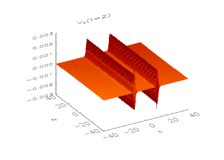
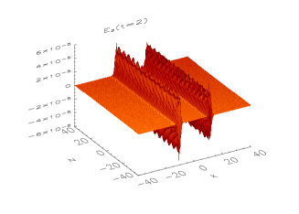
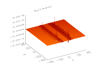
Figure 1: Snapshots of $V_{x}$ and $E_{z}$ at $t=2$ and 20 for the case of $k=10$, $\nu=7$ Hz, $\lambda_{A}=0.63$ Mm.

There were three main stages that lead to the formulation of the present model.

(i) The realisation of the parallel electric field generation (and particle acceleration) being a non-resonant wave-particle interaction effect lead us to the question: could such parallel electric fields be generated in a MHD approximation?

(ii) Next we realised that if one considers non-linear generation of the fast magnetosonic waves in the transversely inhomogeneous plasma, then $\vec{E}=-(\vec{V}\times\vec{B})/c$ contains a non-zero component parallel to the ambient magnetic field $E_{z}=-(V_{x}B_{y}-V_{y}B_{x})/c$.

(iii) From previous studies (Botha et al., 2000; Tsiklauri et al., 2001) we knew that the fast magnetosonic waves ($V_{x}$ and $B_{x}$) did not grow to a substantial fraction of the Alfvén wave amplitude. However after reproducing the old parameter regime (k=1, i.e a frequency of 0.7 Hz), the case of k=10, i.e a frequency of 7 Hz was considered, which showed that fast magnetosonic waves and in turn a parallel electric field were more efficiently generated.

2 model, rationale, and main results

Unlike previous studies (Tsiklauri et al., 2005a, b; Génot et al., 2004, 1999), here we use an ideal MHD description of the problem. We solve numerically ideal, 2.5D, MHD equations in Cartesian coordinates, with a plasma beta of 0.0001 starting from the following equilibrium configuration: A uniform magnetic field $B_{0}$ in the $z-$direction penetrates plasma with the density inhomogeneity across the $x-$direction, which varies according to

$$\rho(x)=\rho_{0}\left[1+2\left(\tanh(x+10)+\tanh(-x+10)\right)\right].$$ (1)

This means that the plasma density increases from some reference background value of $\rho_{0}$, which in our case was fixed at $\rho_{0}=2\times 10^{9}\mu m_{p}$ g cm^-3 (with a molecular weight of $\mu=1.27$ corresponding to the solar coronal conditions ¹H:⁴He=10:1 and $m_{p}$ being the proton mass), to $5\rho_{0}$. Such a density profile across the magnetic field has steep gradients with a half-width of 3 Mm around $x\simeq\pm 10$ Mm and is essentially flat elsewhere. Such a structure mimics e.g. the footpoint of a large curvature radius solar coronal loop or a polar region plume with the ratio of the density inhomogeneity scale and the loop/plume radius of 0.3, which is the median value of the observed range 0.15 - 0.5.

The initial conditions for the numerical simulation are $B_{y}=A\cos(kz)$ and $V_{y}=-c_{A}(x)B_{y}$ at $t=0$, which means that a purely Alfvénic, linearly polarised, plane wave is launched travelling in the direction of positive $z$s. The rest of the physical quantities, $V_{x}$ and $B_{x}$ (which would be components of fast magnetosonic waves if the medium were totally homogeneous) and $V_{z}$ and $B_{z}$ (the analogs of slow magnetosonic waves) are initially set to zero. The plasma temperature is varied as the inverse of Eq.(1) so that the total pressure always remains constant. Boundary conditions used in our simulations are periodic along the $z$- and the zero gradient along the $x$-coordinates. We fixed the amplitude of Alfvén wave $A$ at 0.05 throughout. This choice makes the Alfvén wave weakly non-linear.

As a self-consistency test, we considered situation when the wavenumber of the initial Alfvén wave is $k=1$. In dimensional units this corresponds to an Alfvén wave with frequency ($\nu=0.7$ Hz), i.e. longitudinal wave-numbers $\lambda_{A}=6.3$ Mm. We corroborated the previous results of Botha et al. (2000) and Tsiklauri et al. (2001).

We now present results for the case of large wave-numbers, $k=10$, which in dimensional units correspond to an Alfvén wave with $\nu=7$ Hz, and $\lambda_{A}=0.63$ Mm. This is a regime not investigated before. In Fig. (1) we show shaded surface plots of both the fast magnetosonic waves ($V_{x}$) and parallel electric field $E_{z}$. We gather from this graph that similarly to the results of Tsiklauri et al. (2005b) and Génot et al. (2004), the generated parallel electric field is quite spiky, but more importantly large wave-numbers i.e. short wavelength now are able to significantly increase the amplitudes of both the fast magnetosonic waves ($V_{x}$) and parallel electric field $E_{z}$. This amplitude growth is beyond a simple $A^{2}$ scaling. The amplitude growth is presented quantitatively in Fig. (2) (by doubling spatial resolution we perform satisfactory convergence test). The amplitude of $V_{x}$ now attains values of 0.01 unlike for moderate $k$s. Thus, large wavenumbers (i.e. stronger spatial gradients) seem to yield larger values for the level of saturation of the $V_{x}$ amplitude. In the considered case, $E_{z}$ now attains values of 0.001.

The coronal energy losses that need to be compensated by some additional energy input, to keep the solar corona at the observed temperatures, are (in units of erg cm^-2 s^-1): $3\times 10^{5}$ for the quiet Sun, $8\times 10^{5}$ for a coronal hole and $10^{7}$ for an active region. One can estimate the heating flux per unit area (i.e. in erg cm^-2 s^-1):

$$F_{H}=E_{H}\lambda_{T}=5\times 10^{3}\left(\frac{n_{e}}{10^{8}{\rm cm}}\right)^{2}\left(\frac{T}{1{\rm MK}}\right),$$ (2)

where $E_{H}\approx 10^{-6}$ erg cm^-3 s^-1. This yields an estimate of $F_{H}\approx 2\times 10^{6}$ erg cm^-2 s^-1 in an active region with a typical loop base electron number density of $n_{e}=2\times 10^{9}$ cm^-3 and $T=1$ MK.

The energy density associated with the parallel electric field $E_{z}$ is

$$E_{E}=\frac{\varepsilon E_{z}^{2}}{8\pi},\;\;\;\left[{\rm erg\,cm^{-3}}\right]$$ (3)

where $\varepsilon$ is the dielectric permitivity of plasma. The latter can be deduced from

$$\varepsilon=\frac{4\pi\rho c^{2}}{B^{2}}.$$ (4)

For the coronal conditions ($\rho=2\times 10^{9}\mu m_{p}$ g cm^-3, $\mu=1.27$, $B=100$ Gauss) $\varepsilon\approx 4.8048\times 10^{3}$. In Fig. (2) we saw that electric field amplitude attains a value of $\approx 0.001$. In order to convert this to dimensional units we use $c_{A}^{0}=4328$ km s^-1 and $B=100$ G and $E_{z}=-(V_{x}B_{y}-V_{y}B_{x})/c$ to obtain $E_{z}\approx(c_{A}^{0}B/c)\times 0.001=0.0014$ statvolt cm^-1 (in Gaussian units). Therefore the energy density associated with the parallel electric field $E_{z}$ (From Eq.(3)) is

$$E_{E}=\varepsilon\times 0.0014^{2}/(8\pi)=3.7471\times 10^{-4}$$ (5)

$\left[{\rm erg\,cm^{-3}}\right].$

In order to get the heating flux per unit area for a single harmonic with frequency 7 Hz, we multiply the latter expression by the Alfvén speed of 4328 km s^-1 to obtain

$$F_{E}=E_{E}c_{A}^{0}=1.62\times 10^{5}\;\;\;\left[{\rm erg\,cm^{-2}s^{-1}}\right],$$ (6)

which is $\approx 10$ % of the coronal heating requirement estimate for the same parameters made above using Eq.(2). Note that the latter estimate is for a single harmonic with frequency 7 Hz.

A crucial next step that is needed to understand how the generated electric fields parallel to the uniform unperturbed magnetic field dissipate must invoke kinetic effects. In our two stage model, in the first stage bulk MHD motions (waves) generate the parallel electric fields, which cannot accelerate particles if we describe plasmas in the ideal MHD limit. Génot et al. (2004) and Tsiklauri et al. (2005b) showed that when the identical system is modelled in the kinetic regime particles are accelerated with such parallel fields and Alfvén wave energy is converted into heat on a time scale of a few Alfvén periods.

Figure 2: Time evolution of the amplitudes of $V_{x}\equiv V_{x}^{a}$ and $E_{z}\equiv E_{z}^{a}$. Solid lines with stars represent solutions using the Lare2d code with $4000\times 4000$ resolution, while dash-dotted lines with open symbols are the same but with $2000\times 2000$ resolution. Here $A=0.05$, $k=10$, $\nu=7$ Hz, $\lambda_{A}=0.63$ Mm.

Alfvén waves as observed in situ in the solar wind always appear to be propagating away from the Sun and it is therefore natural to assume a solar origin for these fluctuations. However, the precise origin in the solar atmosphere of the hypothetical source spectrum for Alfvén waves (turbulence) is unknown, given the impossibility of remote magnetic field observations above the chromosphere-corona transition region. Studies of ion cyclotron resonance heating of the solar corona and high speed winds exist which provide important spectroscopic constraints on the Alfvén wave spectrum. Although the spectrum can and is observed at distances of 0.3 AU, it can be projected back to the base of corona using empirical constraints. Therefore, we conjecture that wide spectrum (10${}^{-4}-10^{3}$ Hz) Alfvén waves, based on the observationally constrained spectrum, could provide the necessary coronal heating requirement. The exact amount of energy that could be deposited by such waves through our mechanism of parallel electric field generation can only be calculated once a more complete parametric study is done. Thus, the ”theoretical spectrum” of the energy stored in parallel electric fields versus frequency needs to be obtained. At present we only have two points, 0.7 Hz and 7 Hz, in our ”theoretical spectrum”. Preliminary results will be presented elsewhere (Tsiklauri, 2006a, b).

3 MHD versus kinetic effects and anomalous resistivity

There are two main candidates for the solution of the coronal heating problem: so-called DC and AC models. DC or magnetic reconnection based models need to invoke anomalous resistivity (somewhat ad hoc concept, but there is a lot of indirect evidence for it). At present the details of reconnection in 3D are not understood in full. AC models are often not quantitative, or not enough heating can be provided, unless some enhanced dissipation mechanisms (e.g. phase-mixing, resonant absorption) are invoked. This makes a perfect playground for studying interplay between MHD and kinetic theories of the solar corona. The reason is two-fold: 1) The issue of anomalous resistivity on which DC models rely can only be settled by studying kinetic effects (micro-physics); 2) AC models which use MHD eventually break down, as often system naturally evolves towards progressively small scales (e.g. in phase-mixing); Therefore, kinetic effects become important.

Tsiklauri et al. (2005a, b), amongst other findings, established that the Alfvén wave amplitude decay law in the inhomogeneous regions, in the kinetic regime is $\propto\exp\left[-\left({x\Delta}/{1250\Delta}\right)^{3}\right]$ (where $x$ is the coordinate along uniform magnetic field – mind the change of the geometry!); which is the same as in the MHD approximation discovered by Heyvaerts and Priest (1983) (HP83 thereafter): $\propto\exp\left[-\left(\frac{\eta\omega^{2}V_{A}^{\prime 2}}{6V_{A}^{5}}\right)x^{3}\right]$. Question that begs to be asked: what if we calculate resistivity from the latter MHD formula using our kinetic (PIC) empirical dissipation length of $1250\Delta$? (F. Malara, private communication). By equalising expressions under the both exponents and noting that $x$ from HP83 is equal to $x\Delta$ from our kinetic formula, we obtain $\eta=6V_{A}^{5}/[\omega^{2}V_{A}^{\prime 2}(1250\Delta)^{3}]$. In order to estimate $V_{A}^{\prime}=dV_{A}/dy$ we put $V_{A}^{\prime}\approx V_{A}(y_{*})/\delta y$ where $V_{A}(y_{*})$ is the Alfvén speed at the strongest gradient point and $1/\delta y$ is the strength of the gradient. The latter can be approximated as $(V_{A}(\infty)-V_{A}(0))\delta t/(50\delta)\cdot 1/(50\delta)$, with $50\delta$ being the scale of the transverse density gradient. Putting $\omega=0.3\omega_{ci}$ and $\delta t=54.69/\omega_{ci}$ we obtain $\eta=7\times 10^{-5}V_{A}^{3}(y_{*})\Delta/(V_{A}(\infty)-V_{A}(0))^{2}$. From Tsiklauri et al. (2005a, b) $V_{A}(y_{*})=0.16c$ and $(V_{A}(\infty)-V_{A}(0))=0.25c-0.125c=0.125c$, hence $\eta=1.8\times 10^{-5}c\Delta$. Also, $\Delta=v_{th,e}/\omega_{ce}$. The thermal speed of electrons (at infinity) $v_{th,e}=\sqrt{kT/m_{e}}$, which for 1MK coronal temperature is $3.9\times 10^{8}$ cm s^-1. The electron cyclotron frequency $\omega_{ce}=1.76\times 10^{7}B[G]$, which for 10 G magnetic field is $1.8\times 10^{8}$ s^-1. Thus, $\Delta=2$ cm and we finally obtain $\eta=1.1\times 10^{6}$ cm² s^-1, or in SI units $\eta=1.1\times 10^{2}$ m² s^-1. This is about 100 times greater than the classical Braginskii value for the resistivity. Therefore, the obtained value is a clear indication of the anomalous resistivity. Interestingly others quote similar values for the $\eta$ (Petkaki et al., 2003; Watt et al., 2002).

References

- Botha et al. (2000) Botha G.J.J., Arber T.D., Nakariakov V.M., et al., 2000, A&A 363, 1186
- Chaston et al. (2000) Chaston C.C., Carlson C.W., Ergun R.E., et al., 2000, Phys. Scripta T84, 64
- Génot et al. (2004) Génot V., Louarn P., Mottez F., 2004, Ann. Geophys. 6, 2081
- Génot et al. (1999) Génot V., Louarn P., Le Quéau D., 1999, J. Geophys. Res. 104, 22649
- Hasegawa & Chen (1976) Hasegawa A., Chen L., 1976, Phys. Fluids 19, 1924
- Mottez et al. (2006) Mottez F., Génot V., Louarn P., 2006, A&A 449, 449
- Petkaki et al. (2003) Petkaki P., Watt C.E.J, Horne R.B., et al., 2003, J. Geophys. Res. 108, 1442
- Tsiklauri et al. (2001) Tsiklauri D., Arber T.D., Nakariakov V.M., 2001, A&A 379, 1098
- Tsiklauri et al. (2005a) Tsiklauri D., Sakai J.I., Saito S., 2005, New J. Phys. 7, 79
- Tsiklauri et al. (2005b) Tsiklauri D., Sakai J.I., Saito S., 2005, A&A 435, 1105
- Tsiklauri (2006a) Tsiklauri D., 2006, A&A (in press)
- Tsiklauri (2006b) Tsiklauri D., 2006, New J. Phys. (in press)
- Watt et al. (2002) Watt C.E.J, Horne R.B., Feeman M.P., 2002, Geophys. Res. Lett. 29, 1004