A fresh look on the heating mechanisms of the Solar corona

Abstract

Recently using Particle-In-Cell simulations i.e. in the kinetic plasma description Tsiklauri et al. and Génot et al. reported on a discovery of a new mechanism of parallel electric field generation, which results in electron acceleration. In this work we show that the parallel (to the uniform unperturbed magnetic field) electric field generation can be obtained in much simpler framework using ideal Magnetohydrodynamic (MHD) description, i.e. without resorting to complicated wave particle interaction effects such as ion polarisation drift and resulting space charge separation which seems to be an ultimate cause of the electron acceleration. In the ideal MHD the parallel (to the uniform unperturbed magnetic field) electric field appears due to fast magnetosonic waves which are generated by the interaction of weakly non-linear Alfvén waves with the transverse density inhomogeneity. Further, in the context of the coronal heating problem a new two stage mechanism of the plasma heating is presented by putting emphasis, first, on the generation of parallel electric fields within ideal MHD description directly, rather than focusing on the enhanced dissipation mechanisms of the Alfvén waves and, second, dissipation of these parallel electric fields via kinetic effects. It is shown that a single Alfvén wave harmonic with frequency ($\nu=7$ Hz), (which has longitudinal wavelength $\lambda_{A}=0.63$ Mm for putative Alfvén speed of 4328 km s^-1) the generated parallel electric field could account for the 10% of the necessary coronal heating requirement. We conjecture that wide spectrum (10${}^{-4}-10^{3}$ Hz) Alfvén waves, based on observationally constrained spectrum, could provide necessary coronal heating requirement. It is also shown that the amplitude of generated parallel electric field exceeds the Dreicer electric field by about four orders of magnitude, which implies realisation of the run-away regime with the associated electron acceleration.

During the total solar eclipse of August 7, 1869, Harkness and Young discovered an emission line of feeble intensity in the green part of the spectrum of the corona. Similarly to the case of Helium discovered by Sir Norman Lockyer in 1868 it was mistakenly proposed that this line was due to an unknown element, provisionally named coronium. It was only in 1939 when Grotrian and Edlen correctly identified it as an emission produced by highly ionised Iron at temperatures of a few $\times 10^{6}$ K. Physical understanding of this high temperature in the solar corona is still a fundamental problem in astrophysics. None of the existing models can simultaneously account for all the observational and physical requirements in order to explain what is known as the coronal heating problem.

The second law of thermodynamics states that: It is not possible for heat to flow from a colder body to a warmer body without any work having been done to accomplish this flow. Or energy will not flow spontaneously from a low temperature object to a higher temperature object. This seems to be in apparent contradiction with what we see in the solar atmosphere where temperature steeply rises from the photospheric boundary which is at $T=5785$ K to a few $\times 10^{6}$ K i.e. an increase of a factor of 200. The transition region between the chromosphere (a thin layer above photosphere) and the hot corona over which the temperature increases dramatically is extremely thin ($\approx$ 0.01 % of the Sun’s diameter). This implies that some intense heat deposition occurs in the corona such that the second law of thermodynamics can be saved.

The temperature structure of the solar corona is far from homogeneous Aschwanden (2004). The optically thin emission from the corona in soft X-rays or in the extreme ultra violet implies over-dense structures: so called coronal loops (closed magnetic structures) or plumes in polar regions (open magnetic structures) amongst others. In the corona the thermal pressure is generally much smaller than the magnetic pressure so that their ratio which is known as plasma-$\beta$ parameter is $\ll 1$. This implies that in the corona substantial amount of energy is stored in the magnetic field. In turn, if one could devise a mechanism how this energy is released (dissipated), then important clues to the solution of the coronal heating problem would be revealed.

The coronal heating models are subdivided according to the possibilities of how the currents that are responsible for the plasma heating are dissipated: either by magnetic reconnection Parker (1983); Priest (2003); Priest et al. (2003), Ohmic dissipation via current cascading Ballegooijen (1986); Galsgaard and Nordlund (1996), and viscous turbulence Heyvaerts and Priest (1992) in the case of so called DC models Aschwanden (2004), or by Alfvénic resonance, i.e. resonant absorption Ionson (1978); Ofman et al. (1995); Erdélyi and Goossens (1996); Vasquez and Hollweg (2004), phase mixing Heyvaerts and Priest (1983); Nakariakov et al. (1997); Ruderman et al. (1998); Botha et al. (2000); Tsiklauri et al. (2001); Hood et al. (2002); Tsiklauri and Nakariakov (2002); Tsiklauri et al. (2002, 2003); Tsiklauri et al. (2005b, a), and turbulence Inverarity and Priest (1995) in the case of AC models. An interesting alternative to all of the above models was explored in Tsiklauri (2005), where coronal loops could be heated by the flow of solar wind plasma (plus other flows that may be present) across them by generating currents in a similar manner as a conventional Magnetohydrodynamic (MHD) generator.

Historically all phase mixing studies have been performed in the Magnetohydrodynamic (MHD) approximation, however, since the transverse scales in the Alfvén wave collapse progressively to zero, the MHD approximation is inevitably violated. Thus, Refs.Tsiklauri et al. (2005b, a) studied the phase mixing effect in the kinetic regime, i.e. beyond a MHD approximation, where a new mechanism for the acceleration of electrons due to the generation of parallel electric field in the solar coronal context was discovered. This mechanism has important implications for various space and laboratory plasmas, e.g. the coronal heating problem and acceleration of the solar wind. It turns out that in the magnetospheric context similar parallel electric field generation mechanism in the transversely inhomogeneous plasmas was reported before Génot et al. (2004, 1999) (see also the comment letter Mottez et al. (2006) and references therein).

Contrary to the previous studies Tsiklauri et al. (2005b, a); Génot et al. (2004, 1999), here we use MHD description of the problem. Namely we solve numerically ideal, 2.5D, MHD equations in Cartesian coordinates, with plasma $\beta=0.0001$ starting from the following equilibrium configuration: A uniform magnetic field $B_{0}$ in the $z-$direction penetrates plasma with the density inhomogeneity across $x-$direction, which is varying such that it increases from some reference background value of $\rho_{0}$, which in our case was fixed at $\rho_{0}=2\times 10^{9}\mu m_{p}$ g cm^-3 (with molecular weight of $\mu=1.27$ corresponding to the solar coronal conditions ¹H:⁴He=10:1 Aschwanden (2004) and $m_{p}$ being the proton mass), to $5\rho_{0}$. Such density profile across the magnetic field has steep gradients with half-width of 3 Mm around $x\simeq\pm 10$ Mm and is essentially flat elsewhere. Here ”M” in units stands for mega i.e. $10^{6}$. Such a structure mimics e.g. footpoint of a large curvature radius solar coronal loop or a polar region plume with the ratio of density inhomogeneity scale and the loop/plume radius of 0.3, which is a median value of the observed range 0.15 - 0.5 (Goossens et al., 2002). We use the following usual normalisation $B_{x,y,z}=B_{0}\bar{B}_{x,y,z}$, $(x,y,z)=a_{0}(\bar{x},\bar{y},\bar{z})$, $t=(a_{0}/c_{A}^{0})\bar{t}$. Here $B_{0}$ we fix at 100 G, and hence dimensional Alfvén speed, $c_{A}^{0}=B_{0}/\sqrt{4\pi\rho_{0}}$ turns out to be 4328 km s^-1=0.0144 $c$ ($c$ is the speed of light). The reference length $a_{0}$ was fixed at 1 Mm, i.e. dimensionless time of unity corresponds to 0.2311 s. We usually omit bar on top of normalised quantities, hence when simply numbers are quoted without units, in such circumstances we refer to dimensionless units as defined above. The dimensionless Alfvén speed is normalised to $c_{A}^{0}$. The simulation domain spans from $-40$Mm to 40 Mm in both $x-$ and $z-$directions with the density ramp as described above mimicking a footpoint fragment of a solar coronal loop or a polar region plume. Our initial equilibrium is depicted in Fig. 1.

The initial conditions for the numerical simulation are $B_{y}=A\cos(kz)$ and $V_{y}=-c_{A}(x)B_{y}$ at $t=0$, which means that purely Alfvénic, linearly polarised, plane wave is launched travelling in the direction of positive $z$’s. The rest of physical quantities, namely, $V_{x}$ and $B_{x}$ (which would be components of fast magnetosonic wave if the medium were totally homogeneous) and $V_{z}$ and $B_{z}$ (the analogs of slow magnetosonic wave) are initially set to zero. Plasma temperature is varied as inverse of density so that the total (thermal plus magnetic) pressure always remains constant. We fixed the amplitude of Alfvén wave $A$ at 0.05. This choice makes Alfvén wave weakly non-linear.

The models of coronal heating using wave dissipation were focusing on the mechanisms (e.g. phase mixing) that could enhance damping of the Alfvén waves. However for the coronal value of shear (Braginskii) viscosity, by which Alfvén waves damp of about $\eta=1$ m² s^-1, typical dissipation lengths ($e$-fold decrease of Alfvén wave amplitude over that lengths) are $\simeq 1000$ Mm, only invoking somewhat ad hoc concept of so called enhanced resistivity can bring down the dissipation length to a required value of the order of hydrodynamic pressure scale height $\lambda_{T}\approx 50$ Mm. In this light (observation of mostly undamped Alfvén waves Moran (2001) (see however Ref.O’shea et al. (2005)) and inability of classical (Braginskii) viscosity producing short enough dissipation length), it seems reasonable to focus rather on the generation of parallel electric fields which would guarantee plasma heating should the energy density of the parallel electric fields be large enough. We put emphasis on parallel electric fields because in the direction parallel to the magnetic field electrons (and protons) are not constrained. While in the perpendicular to the magnetic field direction particles are constrained because of large classical conductivity $\sigma=6\times 10^{16}$ s^-1 (for $T=2MK$ corona) and inhibited momentum transport across the magnetic field.

In the MHD limit there are no parallel electric fields associated with the Alfvén wave. In the single fluid, ideal MHD (which is justified because of large $\sigma$) the parallel (to the uniform unperturbed magnetic field) electric field can be obtained from

$$E_{z}=-\frac{V_{x}B_{y}-V_{y}B_{x}}{c}.$$ (1)

This means that in the considered system $E_{z}$ can only be generated if the initial Alfvén wave ($V_{y},B_{y}$) is able to generate fast magnetosonic wave ($V_{x},B_{x}$).

In the recent past, in the context other than parallel electric field generation, Ref. Nakariakov et al. (1997) investigated just such a possibility of growth of fast magnetosonic waves in a similar physical system. They used mostly analytical approach and focused on the early stages of the system’s evolution. Later, long term evolution of the fast magnetosonic wave generation was studied numerically in the case of harmonic Botha et al. (2000) and Gaussian Tsiklauri et al. (2001) Alfvénic initial perturbations. When fast magnetoacoustic perturbations are initially absent and the initial amplitude of the plane Alfvén wave is small, the subsequent evolution of the wave, due to the difference in local Alfvén speed across the $x$-coordinate, leads to the distortion of the wave front. This leads to the appearance of transverse (with respect to the applied magnetic field) gradients, which grow linearly with time. The main negative outcome of the studies with the harmonic Botha et al. (2000) and Gaussian Tsiklauri et al. (2001) Alfvénic initial perturbations was that the amplitudes of $V_{x}$ and $B_{x}$ after rapid initial growth actually tend to saturate due to the destructive wave interference effect Tsiklauri et al. (2001).

We used fully non-linear MHD code Lare2d with the initial conditions as described above. As a self-consistency test we performed numerical simulations with moderate values of $k=1$ (in dimensional units this corresponds to an Alfvén wave with frequency ($\nu=0.7$ Hz), i.e. longitudinal wave-numbers $\lambda_{A}=6.3$ Mm) and corroborated previous results of Botha et al. (2000); Tsiklauri et al. (2001).

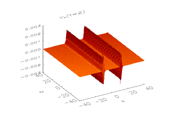
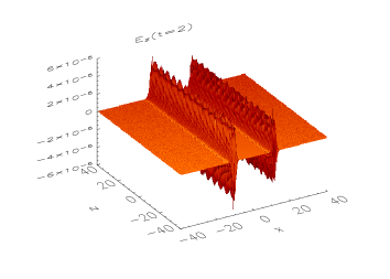
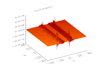
Figure 2: Snapshots of $V_{x}$ and $E_{z}$ at $t=2$ and 20 for the case of $k=10$, $\nu=7$ Hz, $\lambda_{A}=0.63$ Mm.

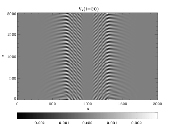
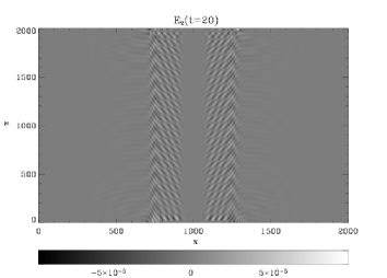
Figure 4: Intensity plots of $V_{x}$ and $E_{z}$ at $t=20$ for the case of $k=1$, $\nu=0.7$ Hz, $\lambda_{A}=6.3$ Mm.

In Fig. (2) we show two snapshots of $V_{x}$ and $E_{z}$ (the latter was reconstructed using Eq.(1)) for the case of $k=10$ (in dimensional units this corresponds to an Alfvén wave with frequency ($\nu=7$ Hz), i.e. longitudinal wave-number $\lambda_{A}=0.63$ Mm.). It can be seen that the fast magnetosonic wave ($V_{x}$) and parallel electric field ($E_{z}$) are both generated in the vicinity of the density gradients $x\simeq\pm 10$, eventually filling the entire density ramp. This means the generated parallel electric fields are confined by the density gradients, i.e. the solar coronal loop (which the considered systems tries to mimic) after about 20 Alfvén time scales becomes filled with the oscillatory in time parallel electric fields. Also, as in Tsiklauri et al. (2005a) and Génot et al. (2004), the generated parallel electric field is quite spiky, but more importantly it seems that large wave-numbers (and frequencies) i.e. short wavelength now are capable to significantly increase the amplitudes of generated both fast magnetosonic waves ($V_{x}$) and parallel electric field $E_{z}$ shown in Fig. (3). In Fig. (3) we plot the amplitudes of $V_{x}\equiv V_{x}^{a}$ and $E_{z}\equiv E_{z}^{a}$ which we define as the maxima of absolute values of the wave amplitudes along $x\simeq\pm 10$ line (which essentially track the generated wave amplitudes in the strongest density gradient regions) at a given time step. This amplitude growth is beyond simple $A^{2}$ scaling (cf. Tsiklauri et al. (2001)). In the considered case $E_{z}$ now attains values of 0.001. To verify the convergence of the solution, we plot the results of the numerical run with the doubled ($4000\times 4000$) spatial resolution. The match seems satisfactory, which validates the obtained results. One could argue that at first sight, the obtained spikes in both fast magnetosonic waves ($V_{x}$) and parallel electric field $E_{z}$ do not contain much energy as they are localised strongly in the wavefront. However, one should realise that in Fig. (2) case of a single harmonic with 7 Hz is considered. If one considers a wide spectrum of Alfvén waves (see discussion of this conjecture below), then the harmonics with different frequencies will contribute to the generation of what will then be a ”forest” of such spikes (for each harmonic). Also, as the frequency of Alfvén waves decreases than much more regular (no longer spiky) wave structures are observed for both fast magnetosonic waves ($V_{x}$) and parallel electric field $E_{z}$. To demonstrate this point we present intensity plots of $V_{x}$ and $E_{z}$ at 20 for the case of $k=1$, $\nu=0.7$ Hz, $\lambda_{A}=6.3$ Mm in Fig. 4. In the latter case the amplitude of $V_{x}$ saturates at $A^{2}=0.05^{2}=0.0025$ as one might expect from the weakly non-linear theory, while $E_{z}$ at $3\times 10^{-5}$.

It has been know for decades Kuperus et al. (1981) that the coronal energy losses that need to be compensated by some additional energy input, to keep solar corona to the observed temperatures, are as following (in units of erg cm^-2 s^-1): $3\times 10^{5}$ for quiet Sun, $8\times 10^{5}$ for a coronal hole and $10^{7}$ for an active region. Ref.Aschwanden (2004) makes similar estimates for the heating flux per unit area (i.e. in erg cm^-2 s^-1):

$$F_{H}=E_{H}\lambda_{T}=5\times 10^{3}\left(\frac{n_{e}}{10^{8}{\rm cm}}\right)^{2}\left(\frac{T}{1{\rm MK}}\right),$$ (2)

where $E_{H}\approx 10^{-6}$ erg cm^-3 s^-1. This yields an estimate of $F_{H}\approx 2\times 10^{6}$ erg cm^-2 s^-1 in an active region of the corona with a typical loop base electron number density of $n_{e}=2\times 10^{9}$ cm^-3 and $T=1$ MK.

In order to make appropriate estimates we first note that the energy density associated with the parallel electric field $E_{z}$ is $E_{E}=\varepsilon E_{z}^{2}/(8\pi)$ erg cm^-3, where $\varepsilon$ is the dielectric permittivity of plasma. The latter can be calculated from $\varepsilon=(4\pi\rho c^{2})/B^{2}$. This expression for $\varepsilon$ is different from the usual expression for the dielectric permittivity Krall and Trivelpiece (1973): $\varepsilon=1+(4\pi\rho c^{2})/B^{2}$ because the displacement current has been neglected in the above treatment, which is a usual assumption made in the MHD limit. At any rate for the coronal conditions ($\rho=2\times 10^{9}\mu m_{p}$ g cm^-3, $\mu=1.27$, $B=100$ Gauss) the second term $(4\pi\rho c^{2})/B^{2}=4.8048\times 10^{3}\approx\varepsilon\gg 1$. ¿From Fig. (3) we gather that the parallel electric field amplitude attains value of $\approx 0.001$. In order to convert this to dimensional units we use $c_{A}^{0}=4328$ km s^-1 and $B=100$ G and Eq.(1) to obtain $E_{z}\approx(c_{A}^{0}B/c)\times 0.001=0.0014$ statvolt cm^-1 (in Gaussian units). Therefore the energy density associated with the parallel electric field $E_{z}$ is $E_{E}=(4.8048\times 10^{3})\times 0.0014^{2}/(8\pi)=3.7471\times 10^{-4}$ erg cm^-3. In order to get the heating flux per unit area for a single harmonic with frequency 7 Hz, we multiply the latter expression by the Alfvén speed of 4328 km s^-1 (this is natural step because the fast magnetosonic waves ($V_{x}$ and $B_{x}$) which propagate across the magnetic field and associated parallel electric fields ($E_{z}$) are generated on density gradients by the Alfvén waves. Hence, the flux is carried with the Alfvén speed) to obtain

$$F_{E}=E_{E}c_{A}^{0}=1.62\times 10^{5}\;\;\;\left[{\rm erg\,cm^{-2}s^{-1}}\right],$$ (3)

which is $\approx 10$ % of the coronal heating requirement estimate for the same parameters made above using Eq.(2). Note that the latter estimate is for a single harmonic with frequency 7 Hz (see discussion below for details when a wide spectrum of Alfvén waves is considered).

We now discuss how the energy stored in the generated parallel electric field is dissipated. For this purpose the parallel electric field behaviour at a given point in space (as a function of time) was studied. We found that $E_{z}$ (in the point of strongest density gradient) is periodic (sign-changing) function which is a mixture of two harmonics with frequencies $\omega=c_{A}k$ and $\omega=2c_{A}k$. This can be qualitatively explained by the fact that $E_{z}$ is calculated using Eq.(1) where $V_{y}$ and $B_{y}$ at fixed spatial point vary in time with frequencies $\omega=c_{A}k$, while the generated $V_{x}$ and $B_{x}$ do so with frequencies $\omega=2c_{A}k$ Nakariakov et al. (1997). Under influence of such periodic parallel electric field electrons start oscillations and are accelerated (while ions perhaps are not due to their larger inertia). It should be emphasised that because of the ideal MHD approximation used in this letter, strictly speaking the generated electric field cannot accelerate plasma particles or cause Ohmic heating unless kinetic effects are invoked. Let us look at the Ohm’s law for ideal MHD (Eq.(1)) in more detail denoting unperturbed by the waves physical quantities with subscript 0 and the ones associated with the waves by a prime: Initial equilibrium implies $\vec{E}_{0}=\vec{V}_{0}=0$ with $\vec{B}_{0}\not=0$. For the perturbed state (with Alfvén waves ($V_{y}$ and $B_{y}$) launched which generate fast magnetosonic waves ($V_{x}$ and $B_{x}$) ) we have

$$\vec{E}^{\prime}=-{\vec{V}^{\prime}\times(\vec{B}_{0}+\vec{B}^{\prime})}/{c}$$ (4)

Note that the projection of $\vec{E}^{\prime}$ on full magnetic field (unperturbed $\vec{B}_{0}$ plus the waves $\vec{B}^{\prime}$) is zero by the definition of cross and scalar product: $\vec{E}^{\prime}\cdot(\vec{B}_{0}+\vec{B}^{\prime})/|(\vec{B}_{0}+\vec{B}^{\prime})|=0$. Physically this means that in ideal MHD electric field cannot do any work as it is always perpendicular to the full (background plus wave) magnetic field. However the projection of $\vec{E}^{\prime}$ on unperturbed magnetic field $\vec{B}_{0}$ is clearly non-zero

$$\vec{E}^{\prime}\cdot\frac{\vec{B}_{0}}{|\vec{B}_{0}|}=E_{z}=-\frac{\vec{V}^{\prime}\times\vec{B}^{\prime}}{c}\cdot\frac{\vec{B}_{0}}{|\vec{B}_{0}|}$$ (5)

which exactly coincides with Eq.(1) that was used to calculate $E_{z}$ throughout this letter. Crucial next step needed to understand how the generated parallel (to the uniform unperturbed magnetic field) electric fields dissipate must invoke kinetic effects. In our two stage model, in the first stage bulk MHD motions (waves) are generating the parallel electric fields, which as we saw cannot accelerate particles if we describe plasmas in the ideal MHD limit. Clearly we witnessed in works of Génot et al. (2004) and Tsiklauri et al. (2005a) that when identical system is modelled in kinetic regime particles are indeed accelerated with such parallel fields. Génot et al. (2004) claimed that electron acceleration is due to the polarisation drift. In particular, they showed that once Alfvén wave propagates on the transverse to the magnetic field density gradient, parallel electric field is generated due to charge separation caused by the polarisation drift associated with the time varying electric field of the Alfvén wave. Because polarisation drift speed is proportional to the mass of the particle, it is negligible for electrons, hence ions start to drift. This causes charge separation (the effect that is certainly beyond reach of MHD description), which results in generation of the parallel electric fields, that in turn accelerates electrons. In the MHD consideration our parallel electric field is also time varying, hence at the second (kinetic) stage the electron acceleration can proceed in the same manner through the ion polarisation drift and charge separation. The exact picture of the particle dynamics in this case can no longer be treated with MHD and kinetic description is more relevant. It should be mentioned that the frequencies considered in kinetic regime (Tsiklauri et al., 2005a), $\nu=0.3\omega_{ci}/(2\pi)=4.6\times 10^{4}$ Hz and this letter, $0.7-7$ Hz, are different, but we clearly saw that the increase in frequency just yields enhancement of the parallel electric field generation. Various effects of wave-particle interactions will rapidly damp the parallel electric fields on a time scale much shorter than MHD time scale. Génot et al. (2004) clearly demonstrated the role of nonlinearity and kinetic instabilities in the rapid conversion from initial low frequency electromagnetic regime, to a high frequency electrostatic one. They identified Buneman and weak beam plasma instabilities in their simulations (as they studied time evolution of the system for longer than Tsiklauri et al. (2005a) times). Fig.(11) from Génot et al. (2004) shows that wave energy is converted into particle energy on the times scales of $10^{3}\omega_{pe}^{-1}\approx 4$ Alfvén periods. Perhaps no immediate comparison is possible (because of the different frequencies involved), but still in our case Alfvén period when sufficient energy is stored in the parallel electric field is $1/(7$ Hz)=0.14 s, i.e. wave energy is converted into the particle energy in quite short time.

Our aim here was to show that parallel electric field generation is possible even within the MHD framework without resorting to plasma kinetics. Yet another important observation can be made by estimating the Dreicer electric field Dreicer (1959). Dreicer considered dynamics of electrons under action of two effects: the parallel electric field and friction between electrons and ions. He noted that the equation describing electron dynamics along the magnetic field can be written as

$$m_{e}\dot{v_{d}}=eE-\nu_{p}^{e/i}m_{e}v_{d}$$ (6)

where $v_{d}$ is the electron drift velocity and $\nu_{p}^{e/i}$ is the electron collision frequency and dot denotes time derivative. We note in passing that when $v_{d}\ll v_{thermal}$ Eq.(6) in the steady state regime ($d/dt=0$) allows to derive the expression for Spitzer resistivity. When $v_{d}>v_{thermal}$ then steady state solution may not apply. In this case when the right hand side of Eq.(6) is positive i.e. when $eE>\nu_{p}^{e/i}m_{e}v_{d}$, we have electron acceleration. In fact this is so called run-away regime. In simple terms acceleration due to parallel electric field leads to an increase in $v_{d}$, in turn, this leads to decrease in $\nu_{p}^{e/i}$ because $\nu_{p}^{e/i}\propto 1/v_{d}^{3}$. In other words when electric field exceeds the critical value $E_{d}=n_{e}e^{3}\ln\Lambda/(8\pi\varepsilon_{0}^{2}k_{B}T)$ (the Dreicer electric field, which is quoted here in SI form), faster drift leads to decrease in electron-ion friction, which in turn results in even faster drift speed and hence run-away regime is reached. Putting in coronal values ($n_{e}=2\times 10^{9}$ cm^-3, $T=1$ MK and $\ln\Lambda=17.75$) in the expression for the Dreicer electric field we obtain 0.0054 V m^-1 which in Gaussian units is $1.8\times 10^{-7}$ statvolt cm^-1. As can be seen from this estimate the values of parallel electric field obtained in this letter exceeds the Dreicer electric field by about four orders of magnitude! This guarantees that ran-away regime would take place leading to the electron acceleration and fast conversion of the generated electric field energy in to heat. It should be noted, however, that in Eq.(6) $E$ is constant, while our $E_{z}$ in the point of strongest density gradient is time varying. Hence some modification from the Dreicer analysis is expected.

It has been known for decades that the flux carried by Alfvén waves in the solar corona is more than enough to heat it to the observed temperatures Kuperus et al. (1981), however linear MHD Alfvén waves in homogeneous plasma do not possess parallel electric field component. This is one of the reasons why they are so difficult to dissipate. Hence the novelty of this study was to consider situation when parallel electric field generation is possible (weak non-linearity and transverse density inhomogeneity).

After comment paper by Mottez et al. (2006) we came to realisation that electron acceleration seen in both series of works (Tsiklauri et al., 2005b, a; Génot et al., 2004, 1999) is a non-resonant wave-particle interaction effect. In works by Tsiklauri et al. (2005b, a) electron thermal speed was $v_{th,e}=0.1c$ while Alfvén speed in the strongest density gradient regions was $v_{A}=0.16c$, this unfortunate coincidence led us then to the conclusion that the electron acceleration by parallel electric fields was affected by the Landau resonance with the phase mixed Alfvén wave. In works by (Génot et al., 2004, 1999) electron thermal speed was $v_{th,e}=0.1c$ while Alfvén speed was $v_{A}=0.4c$ because they considered more strongly magnetised plasma applicable to Earth magnetospheric conditions. There were three main stages that lead to the formulation of the present model.

(i) The realisation of the parallel electric field generation (and particle acceleration) being a non-resonant wave-particle interaction effect, lead us to a question: could such parallel electric fields be generated in MHD approximation?

(ii) Next we realised that indeed if one considers non-linear generation of fast magnetosonic waves in the plasma with transverse density inhomogeneity, then $\vec{E}=-(\vec{V}\times\vec{B})/c$ contains non-zero component parallel to the ambient magnetic field $E_{z}=-(V_{x}B_{y}-V_{y}B_{x})/c$.

(iii) From previous studies (Botha et al., 2000; Tsiklauri et al., 2001) we knew that the fast magnetosonic waves ($V_{x}$ and $B_{x}$) did not grow to a substantial fraction of the Alfvén wave amplitude. However after reproducing old parameter regime (k=1, i.e frequency of 0.7 Hz), fortunately case of k=10, i.e frequency of 7 Hz was considered, which showed that fast magnetosonic waves and in turn parallel electric field were more efficiently generated.

We close this letter with the following four points:

(i) In this work we showed that the parallel electric field generation reported in number of previous publications Tsiklauri et al. (2005b, a); Génot et al. (2004, 1999) which dealt with transversely inhomogeneous plasma can be explained in much simpler framework using MHD description, i.e. without resorting to complicated wave particle interaction effects.

(ii) In the context of the coronal heating problem a new two stage mechanism of the plasma heating is presented by putting emphasis, first, on the generation of parallel electric fields within ideal MHD description directly, rather than focusing on the enhanced dissipation mechanisms of the Alfvén waves and, second, dissipation of these parallel electric fields via kinetic effects.

(iii) It is shown that a single Alfvén wave harmonic with frequency ($\nu=7$ Hz), (which has longitudinal wavelength $\lambda_{A}=0.63$ Mm for putative Alfvén speed of 4328 km s^-1) the generated parallel electric field could account for the 10% of the necessary coronal heating requirement. We conjecture that the wide spectrum (10${}^{-4}-10^{3}$ Hz) Alfvén waves, based on observationally constrained spectrum, could provide necessary coronal heating requirement. In this regard, it should mentioned that Alfvén waves as observed in situ in the solar wind always appear to be propagating away from the Sun and it is therefore natural to assume a solar origin for these fluctuations. However, the precise origin in the solar atmosphere of the hypothetical source spectrum for Alfvénic waves (turbulence) is unknown, given the impossibility of remote magnetic field observations above the chromosphere-corona transition region (Velli and Pruneti, 1997). Studies of ion cyclotron resonance heating of the solar corona and high speed winds exist which provide important spectroscopic constraints on the Alfvén wave spectrum (Cranmer et al., 1999). Although the spectrum can and is observed at distances of 0.3 AU, it can be then projected back at the base of corona using empirical constraints, see e.g. top line in Fig. 5 from Cranmer et al. (1999). Using the latter figure we can make the following estimates. Let us look at single harmonic, first. At frequency 7 Hz (used in our simulations) magnetic energy of Alfvénic fluctuations is $E_{\nu}^{(\rm 7\,Hz)}\approx 10^{7}$ nT² Hz^-1. For single harmonic with $\nu=7$ Hz this gives for the energy density $E^{(\rm 7\,Hz)}\equiv\nu E_{\nu}^{(\rm 7\,Hz)}/(8\pi)\approx 7\times 10^{-3}$ G${}^{2}/(8\pi)\approx 2.8\times 10^{-4}$ erg cm^-3. Note that surprisingly this semi-observational value is quite close to our theoretical value of $3.7471\times 10^{-4}$ erg cm^-3! As we saw above such single harmonic can provide approximately 10 % of the coronal heating requirement. Next let us look at how much energy density is stored in Alfvén wave spectrum based on empirically guided top line in Fig. 5 from Cranmer et al. (1999). Their spectral energy density (which they call ”power”) is approximated by so called $1/f$ spectrum, i.e. $E_{\nu}=0.6\times 10^{8}/\nu$ nT² Hz^-1. Which in proper energy density units is $E_{\nu}=2.4\times 10^{-4}/\nu$ erg cm^-3 Hz ^-1. Hence the flux carried by Alfvén waves from say $10^{-4}$ Hz up to a frequency $\nu$ would be

$$F^{\rm AW}=\int_{10^{-4}\,{\rm Hz}}^{\nu}E_{\nu}c_{A}^{0}d\nu=1.04\times 10^{5}\ln(\nu/10^{-4})$$ (7)

$\left[{\rm erg\,cm^{-2}s^{-1}}\right]$. Based on the latter equation we deduce that the Alfvén wave spectrum from $\nu=10^{-4}$ Hz up to about few $\times 10^{3}$ Hz carries a flux that is nearly as much as the coronal heating requirement, $F_{H}\approx 2\times 10^{6}$ erg cm^-2 s^-1, quoted above. We refrain from considering higher frequencies because for about $10^{4}$ Hz ions become resonant with circularly polarised Alfvén waves and the dissipation proceeds through the Landau resonance – the well studied mechanism, but quite different from our non-resonant mechanism of parallel electric field generation.

There are several possibilities how this flux carried by Alfvén waves (fluctuations), is dissipated. If we consider regime of frequencies up to $10^{3}$ Hz, ion cyclotron resonance condition is not met and hence dissipation would be dominated through the mechanism of parallel electric field dissipation formulated in this letter. However at this stage it is unclear how much energy could actually be dissipated. This is due to the fact that we only have two points 0.7 Hz and 7 Hz in our ”theoretical spectrum”. As we saw a single Alfvén wave harmonic with frequency 7 Hz can dissipate enough heat to account for 10% of the coronal heating requirement. Therefore, we conjecture that wide spectrum (10${}^{-4}-10^{3}$ Hz) Alfvén waves, based on observationally constrained spectrum, could provide necessary coronal heating requirement. More details on the issue of wide spectrum will be published elsewhere Tsiklauri (2006).

(iv) The obtained value of the generated parallel electric field exceeds the Dreicer electric field by about four orders of magnitude, which implies realisation of the run-away regime with the associated electron acceleration.

acknowledgements Author kindly acknowledges support from the Nuffield Foundation (UK) through an award to newly appointed lecturers in Science, Engineering and Mathematics (NUF-NAL 04) and from the University of Salford Research Investment Fund 2005 grant. Author acknowledges use of E. Copson Math cluster funded by PPARC and University of St. Andrews. Author also would like to thank two anonymous referees for the comments that improved this letter.

Figure 1: Dimensionless density ($\rho(x)/\rho_{0}=\left[1+2\left(\tanh(x+10)+\tanh(-x+10)\right)\right]$) (solid line) and Alfvén speed, ($c_{A}(x)=1/\sqrt{1+2\left(\tanh(x+10)+\tanh(-x+10)\right)}$) (dashed line) profiles across the uniform unperturbed magnetic field (i.e. along $x$-coordinate) which is used as an equilibrium configuration in our model of a footpoint of a solar coronal loop or a solar polar region plume.

Figure 3: Time evolution of the amplitudes of $V_{x}\equiv V_{x}^{a}$ and $E_{z}\equiv E_{z}^{a}$. Solid lines with stars represent solutions using the Lare2d code with $4000\times 4000$ resolution, while dash-dotted lines with open symbols are the same but with $2000\times 2000$ resolution. Here $k=10$, $\nu=7$ Hz, $\lambda_{A}=0.63$ Mm.

References

- Aschwanden (2004) M. J. Aschwanden, Physics of the solar corona an introduction (Praxis Publishing Ltd, Chichester, UK, 2004).
- Parker (1983) E. N. Parker, Astrophys. J. 264, 642 (1983).
- Priest (2003) E. R. Priest, Adv. Space Res. 32, 1021 (2003).
- Priest et al. (2003) E. R. Priest, D. W. Longcope, and V. S. Titov, Astrophys. J. 598, 667 (2003).
- Ballegooijen (1986) A. A. V. Ballegooijen, Astrophys. J. 311, 1001 (1986).
- Galsgaard and Nordlund (1996) K. Galsgaard and A. Nordlund, J. Geophys. Res. 101, 13445 (1996).
- Heyvaerts and Priest (1992) J. Heyvaerts and E. R. Priest, Astrophys. J. 390, 297 (1992).
- Ionson (1978) J. A. Ionson, Astrophys. J. 226, 650 (1978).
- Ofman et al. (1995) L. Ofman, J. M. Davila, and R. S. Steinolfson, Astrophys. J. 444, 471 (1995).
- Erdélyi and Goossens (1996) R. Erdélyi and M. Goossens, Astron. Astrophys. 313, 664 (1996).
- Vasquez and Hollweg (2004) B. J. Vasquez and J. V. Hollweg, Geophys. Res. Lett. 31, L14803 (2004).
- Heyvaerts and Priest (1983) J. Heyvaerts and E. R. Priest, Astron. Astrophys. 117, 220 (1983).
- Nakariakov et al. (1997) V. M. Nakariakov, B. Roberts, and K. Murawski, Sol. Phys. 175, 93 (1997).
- Ruderman et al. (1998) M. S. Ruderman, V. M. Nakariakov, and B. Roberts, Astron. Astrophys. 338, 1118 (1998).
- Botha et al. (2000) G. J. J. Botha, T. D. Arber, V. M. Nakariakov, and F. P. Keenan, Astron. Astrophys. 363, 1186 (2000).
- Tsiklauri et al. (2001) D. Tsiklauri, T. D. Arber, and V. M. Nakariakov, Astron. Astrophys. 379, 1098 (2001).
- Hood et al. (2002) A. W. Hood, S. J. Brooks, and A. N. Wright, Proc. Roy. Soc. Lond. A 458, 2307 (2002).
- Tsiklauri and Nakariakov (2002) D. Tsiklauri and V. M. Nakariakov, Astron. Astrophys. 393, 321 (2002).
- Tsiklauri et al. (2002) D. Tsiklauri, V. M. Nakariakov, and T. D. Arber, Astron. Astrophys. 395, 285 (2002).
- Tsiklauri et al. (2003) D. Tsiklauri, V. M. Nakariakov, and G. Rowlands, Astron. Astrophys. 400, 1051 (2003).
- Tsiklauri et al. (2005a) D. Tsiklauri, J. I. Sakai, and S. Saito, Astron. Astrophys. 435, 1105 (2005a).
- Tsiklauri et al. (2005b) D. Tsiklauri, J. I. Sakai, and S. Saito, New J. Phys. 7, 79 (2005b).
- Inverarity and Priest (1995) G. W. Inverarity and E. R. Priest, Astron. Astrophys. 302, 567 (1995).
- Tsiklauri (2005) D. Tsiklauri, Astron. Astrophys. 441, 1177 (2005).
- Génot et al. (2004) V. Génot, P. Louarn, and F. Mottez, Ann. Geophys. 6, 2081 (2004).
- Génot et al. (1999) V. Génot, P. Louarn, and D. L. Quéau, J. Geophys. Res. 104, 22649 (1999).
- Mottez et al. (2006) F. Mottez, V. Génot, and P. Louarn, Astron. Astrophys. 449, 449 (2006).
- Goossens et al. (2002) M. Goossens, J. Andries, and M. J. Aschwanden, Astron. Astrophys. 394, L39 (2002).
- Moran (2001) T. G. Moran, Astron. Astrophys. 374, L9 (2001).
- O’shea et al. (2005) E. O’shea, D. Banerjee, and J. G. Doyle, Astron. Astrophys. 436, L35 (2005).
- Kuperus et al. (1981) M. Kuperus, J. A. Ionson, and D. S. Spicer, Ann. Rev. Astron. Astrophys. 19, 7 (1981).
- Krall and Trivelpiece (1973) N. A. Krall and A. W. Trivelpiece, Principles of Plasma Physics (McGraw-Hill, New York, 1973).
- Dreicer (1959) H. Dreicer, Phys. Rev. 115, 238 (1959).
- Velli and Pruneti (1997) M. Velli and F. Pruneti, Plasma Phys. Control. Fusion 39, B317 (1997).
- Cranmer et al. (1999) S. R. Cranmer, G. B. Field, and J. L. Kohl, Astrophys. J. 518, 937 (1999).
- Tsiklauri (2006) D. Tsiklauri, Astron. Astrophys. (submitted) (2006).