Eclipsing binaries observed with the wire satellite

Abstract

Context. Determinations of stellar mass and radius with realistic uncertainties at the level of 1% provide important constraints on models of stellar structure and evolution.

Aims. We present a high-precision light curve of the A0 IV star $\psi$ Centauri, from the star tracker on board the wire satellite and the Solar Mass Ejection Imager camera on the Coriolis spacecraft. The data show that $\psi$ Cen is an eccentric eclipsing binary system with a relatively long orbital period.

Methods. The wire light curve extends over 28.7 nights and contains 41 334 observations with 2 mmag point-to-point scatter. The eclipse depths are 0.28 and 0.16 mag, and show that the two eclipsing components of $\psi$ Cen have very different radii. As a consequence, the secondary eclipse is total. We find the eccentricity to be $e=0.55$ with an orbital period of 38.8 days from combining the wire light curve with data taken over two years from the Solar Mass Ejection Imager camera.

Results. We have fitted the light curve with ebop and have assessed the uncertainties of the resulting parameters using Monte Carlo simulations. The fractional radii of the stars and the inclination of the orbit have random errors of only 0.1% and 0.01^∘, respectively, but the systematic uncertainty in these quantities may be somewhat larger. We have used photometric calibrations to estimate the effective temperatures of the components of $\psi$ Cen to be $10\,450\pm 300$ and $8\,800\pm 300$ K indicating masses of about 3.1 and 2.0$\,{\rm M}_{\odot}$. There is evidence in the wire light curve for $g$-mode pulsations in the primary star.

1 Introduction

The study of detached eclipsing binaries is of fundamental importance to stellar astronomy as a means by which we can measure accurately the parameters of normal stars from basic observational data (Andersen andersen91 (1991)). The masses and radii of the component stars of a detached eclipsing binary (dEB) can be measured to accuracies better than 1% (e.g. Southworth et al., SMS05 (2005)), and the effective temperatures and luminosities can be obtained from spectral analysis or the use of photometric calibrations. An important use of these data is in the calibration of theoretical models of stellar evolution (Pols et al. pols+97 (1997); Andersen et al. andersen1990 (1990); Ribas et al. ribas+00 (2000)). Comparing the properties of a dEB to the predictions of theoretical models allows the age and metal abundance of the binary to be estimated (e.g. Southworth et al. 2004a ) and the accuracy of the predictions to be checked, particularly if the two components of the dEB are of quite different mass or evolutionary stage (e.g. Andersen et al. andersenetal1991 (1991)).

Some of the physical effects contained in current theoretical stellar evolutionary models are poorly understood, so are treated using simple parameterisations, for example convective core overshooting and convective efficiency (mixing length). Whilst these parameterisations provide a good way of including such physics, our incomplete knowledge of their parameter values is compromising the predictive power of the models (Chaboyer chaboyer95 (1995), Young et al. young01 (2001)) and must be improved. The amount of convective core overshooting has been studied using dEBs by Andersen et al. (andersen1990 (1990)) and Ribas et al. (ribas+00 (2000)), and the mixing lengths in the binary AI Phœnicis has been determined by Ludwig & Salaris (ludwig+99 (1999)), but these studies have not been able to provide definitive answers because the age and chemical composition are usually free parameters which can be adjusted when comparing the model predictions to the properties of the dEBs.

Progress in the calibration of convective overshooting and mixing length may be made by increasing the accuracy with which the basic parameters of dEBs are measured, which requires much improved observational data. It is arguably more difficult to significantly improve the quality and quantity of light curves, rather than radial velocity curves, because a large amount of telescope time is needed for each system. Forthcoming space missions such as kepler (Basri et al. kepler05 (2005)) and corot (Baglin et al. baglin01 (2001)) will help to solve this problem by obtaining accurate and extensive light curves of a significant number of dEBs.

We have begun a programme to obtain high-quality photometry of bright dEBs with the Wide field InfraRed Explorer (wire) satellite, with the intention of measuring the radii of the component stars to high accuracy. Several of the targets in this program have long orbital periods ($\psi$ Cen) or shallow eclipses (AR Cas; Southworth et al. (2006)) which has made them difficult to observe using ground-based telescopes. $\psi$ Cen and AR Cas have secondary components which have much smaller masses and radii than the primary stars, so will be able to provide strict constraints on the predictions of theoretical models. An additional advantage of having components with very different radii is that the eclipses are nearly total, which generally allows the radii to be measured with increased accuracy compared to systems with partial eclipses.

In this paper we report our discovery of eclipses in the bright ($V=4.1$) A0 IV star $\psi$ Cen made with the wire satellite. We present a detailed analysis of the light curve showing that the orbit is eccentric and the secondary eclipse is total. As is turns out, this is a particularly interesting system since its brightest component is located in the region of the Hertzsprung-Russell diagram between the blue edge of the Cepheid instability strip and the region of $g$-mode oscillations seen in slowly pulsating B stars (see, e.g., Pamyatnykh pamyat1999 (1999)). We present an analysis of the oscillations showing evidence of two low-frequency modes that may be interpreted as global oscillation $g$-modes in the primary star.

2 Photometry from space: wire, smei and hipparcos

Since 1999 the star tracker on the wire satellite (Hacking et al. hacking99 (1999)) has been used to observe around 250 stars which have apparent magnitudes $V<7$ (see Bruntt et al. bruntt05 (2005)). The aperture is 52 $m$m and data is acquired at a cadence of 2 Hz. Each star is monitored for typically 2–4 weeks and some targets have been observed in more than one season. The primary aim has so far been to map the variability of stars of all spectral types, and recently we have done coordinated ground- and space-based observations. When planning the wire observations a primary target is chosen and in addition the on-board computer selects four additional bright stars within the field of view (FOV) of 8.5^∘ by 8.5^∘. The monitoring of five stars by the star tracker was originally designed to perform accurate attitude control. The rms uncertainty on the position is 0.0085 pixels or about 0.5 arc seconds.

When binning data to one point every 15 seconds the rms uncertainty per data point is 0.3 and 5 mmag for a $V=0$ and $6$ star, respectively. The filter response of wire is not well known. From an analysis of the light collected from stars of various spectral types and measured brightness we estimate the filter to approximate Johnson $V+R$. The amplitudes of variation of variable stars studied from the ground and with wire are in rough agreement with this, e.g. Bruntt et al. (2006) compared Strömgren $y$ and wire filter observations of the same $\delta$ Scuti star.

The orbital period of wire, which has been slowly decreasing since its launch in 1999, was 93.8 minutes at the time of these observations. wire switches between two targets during each orbit in order to best avoid the illuminated face of the Earth. Consequently, the duty cycle is typically around 20–30% or about 19–28 minutes of continuous observations per orbit.

The A0 IV type-star $\psi$ Cen was observed nearly continuously for 28.7 days from June 11 to July 9 2004 as one of the secondary targets for the bright giant star $\theta$ Cen. After binning the light curve to a time sampling of 15 seconds we have 41 334 data points with a point-to-point scatter of only 2.1 mmag. The light curve shows only one primary and one secondary eclipse separated in time by about 7 days, indicating that the orbit is eccentric and has a long period. The depths of the eclipses are about 0.28 mag for the primary and 0.16 mag for the secondary, indicating that the components have quite different surface fluxes. The phased light curve from wire is shown in Fig. 1.

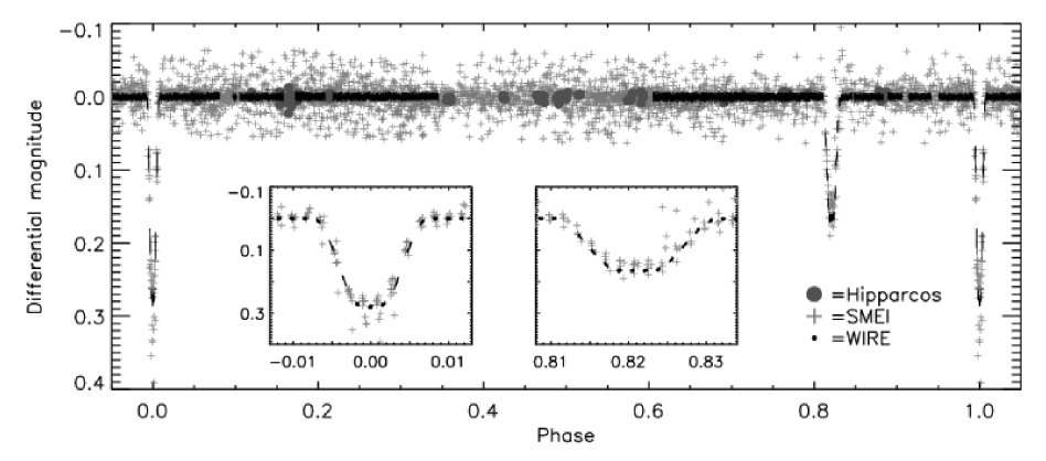
Figure 1: Phased light curve of $\psi$ Cen for a period of 38.81252 days. Data points from wire (black dots), smei (grey $+$ symbols), and hipparcos (grey circles) are shown.

The wire data only contain one primary and one secondary eclipse, so cannot be used to find the orbital period of $\psi$ Cen. We therefore obtained data from the Solar Mass Ejection Imager (smei) camera on the Coriolis satellite. smei is an all-sky camera aboard the U.S. Department of Defense Space Test program’s Coriolis satellite which was launched on January 6 2003 into a 840 km high Sun-synchronous polar orbit. The primary purpose of smei is to detect and track transient structures, such as coronal mass ejections emanating from the Sun by observing Thomson-scattered sunlight from heliospheric plasma (see Webb et al. webb06 (2006)). Jackson et al. (2004) provide the history of the smei design and development, and the instrument design and testing are described by Eyles et al. (2003). A description of its performance is given in Webb et al. (webb06 (2006)).

smei consists of 3 CCD cameras each with an asymmetrical aperture of 1.76 cm² area and viewing a 3 x 60 degree strip of the sky, aligned end-to-end and slightly overlapping so as to provide a 3 degree wide strip extending approximately 160 degrees along a great circle with one end near the direction of the Sun and the other at the anti-Sun direction. The cameras are fixed on the zenith-nadir pointing Coriolis satellite, pointing some 30 degrees above the rear Earth horizon. Thus, during each 102 minute orbit of the satellite the cameras are swept to cover about 90% of the entire sky, with a duty cycle of about 85% from launch until the present (March 2006). The unfiltered bandpass has a response which rises above 10% between 450 and 950 nm, with a peak response of about 50%, thus corresponding roughly to a wide $R$ photometric band. A G-type star with $V=10$ viewed on-axis produces approximately 800 photo-electrons during a single 4 s exposure. Each camera takes an image every 4 seconds (which are thus smeared roughly by 0.2 degrees across the picture). The camera pointing nearest the Sun (Camera 3) is used in a mode that gives it $0.1\times 0.1$ degree binned pixels, whilst for the other two the binned pixels are $0.2\times 0.2$ degrees. The very fast (f/1.2$\times$f/2.2) optics are used to give a point spread function (PSF), with a full-width at half-maximum of about 0.08 degrees but with wide wings. Whilst for the main project aim, the optical design is very suitable, for the aim of stellar photometry there are certain drawbacks, namely the short exposures, the optical distortion of the FOV and of the PSF, the large pixel size, and the variation of the CCD temperatures during an orbit. The main limitation, however, is the crowding.

We used smei data covering two years from March 21 2003 to March 15 2005. Using only one of the three cameras (Camera 2) for these preliminary studies, the data have gaps varying between 87 and 140 days when the star is visible only in one of the other two cameras. The typical accuracy per data point is about 16 mmag, which is significantly larger than the wire accuracy of 2.1 mmag. We have 3 773 data points from smei but a significant fraction are spurious outliers (see Sect. 2.1). The grey points in the phased light curve in Fig. 1 are the smei data.

We also used 91 data points from hipparcos (ESA (1997)) collected from February 1990 to February 1993. Whilst none of these data points were taken during eclipse, they have been useful in helping to constrain the period of $\psi$ Cen.

Figure 2: The wire light curve during the primary and secondary eclipses is compared to the best-fitting ebop model (dotted line). The residuals of the fit are shown below each panel with an increased scale. In these plots groups of five points were binned together.

2.1 Data reduction

The wire dataset consists of about 1.3 million windows extracted from the 512$\times$512 CCD star tracker camera. Each window is 8$\times$8 pixels and aperture photometry is carried out. The basic data reduction was done using the pipeline described by Bruntt et al. (bruntt05 (2005)).

In the smei dataset $\psi$ Cen will appear on approximately 30 out of the 20 000 images from each satellite orbit. For about 15 of these, the star will be adequately distant from the FOV edges (giving a total exposure in each orbit of about one minute). For each image used, the CCD data have bias and dark current removed. The dark flux for each pixel varies from exposure to exposure as the camera temperature changes. The significant variation in effective telescope aperture with off-axis direction is allowed for. Glare from scattered sunlight is subtracted using an empirical map (Buffington, private communication, 2006). Further details of the glare are given in Buffington et al. (2005). From the satellite pointing information each pixel in an approximately $1.2\times 1.2$ degree area around the star is given an absolute sky direction, accurate to a few arc seconds. Then for all the binned pixels used (about 500) a PSF is fitted by a linearised least-squares method to derive the height and sloping base. The PSF is empirically determined from observations of Sirius taken when the cameras are being used in an optional $0.05\times 0.05$ degree pixel high-resolution mode. Full details of the data reduction are planned to be given in Penny et al. (2006). Further discussion of stellar photometry with smei is also given in Buffington et al. (2006).

The smei data contain a significant number of spurious outliers and for the subsequent analysis we removed these. Initially we used all data points to determine the approximate period. After phasing the data points with this period, we discarded data points that deviate more than 3.5 $\sigma$ or 64 mmag, but only for data points outside the times of eclipse. During times of eclipse we removed only five data points that deviated more than 150 mmag from the mean phased light curve. A total of 325 spurious data points, or about $9\%$ of the smei data, were discarded.

The hipparcos photometry was extracted directly from the vizier database. The 91 data points from hipparcos have a mean magnitude of $H_{\rm p}=4.039\pm 0.004$. The mean magnitude outside eclipse was subtracted from each of the wire, smei and hipparcos prior to subsequent analysis.

A small part of the wire light curve is given in Table 1 while the complete dataset from both wire and smei is available in electronic format at Centre de Données astronomiques de Strasbourg (CDS).

Table 1: wire and smei observations of $\psi$ Cen. The magnitudes for each source have been normalised so the outside-eclipse magnitude is zero. The full table comprises 44 782 datapoints and is available at the CDS.

HJD $-$ 2400000	Magnitude	Source
53167.7383428	0.000022	WIRE
53167.7385222	$-$0.000355	WIRE
53167.7387016	0.002896	WIRE
53167.7388847	$-$0.000195	WIRE
53167.7390662	$-$0.000541	WIRE
53167.7392467	0.000129	WIRE
53167.7394309	$-$0.001556	WIRE
53167.7396159	0.000402	WIRE
53167.7397979	$-$0.001407	WIRE
53167.7399805	$-$0.001965	WIRE

3 Light curve analysis

The high quality of the wire light curve of $\psi$ Cen has allowed us to derive extremely precise photometric parameters for the stars. The orbital period of $\psi$ Cen is not determined from the wire data, which only contains one primary and one secondary eclipse for this eccentric system, so we have included the smei data in our analysis as they contain observations during eclipses separated by up to two years.

Preliminary times of minimum light were derived from the smei and wire data by fitting Gaussian functions to the eclipses present in the data. An orbital period of 38.8119(9) days provides a good fit to these times of minima and the overall light curve of $\psi$ Cen. The actual shape of the eclipses are however, quite non-Gaussian, and therefore the orbital period and the reference time of the central primary eclipse were included as fitting parameters in the light curve analysis. As seen in Table 2 we obtained a period of 38.81252(29) days. The phased light curve is shown in Fig. 1 and the details of the eclipses seen with wire are shown in Fig. 2.

The wire and smei light curves were analysed with jktebop (Southworth et al. 2004b , 2004c ), which uses the NDE eclipsing binary model (Nelson & Davis nelson72 (1972)) as implemented in the ebop code (Etzel etzel81 (1981); Popper & Etzel popper81 (1981)). This model represents the projected shapes of the components of an eclipsing binary as biaxial spheroids, an approximation which is easily adequate for $\psi$ Cen, whose components are almost spherical. A significant advantage of the model is that it involves very few calculations, meaning that extensive error analyses can be undertaken quickly using standard computing equipment. For this application, jktebop was modified to allow the orbital period and time of primary mid-minimum to be included as free parameters.

Preliminary solutions of the wire and smei datasets were made using jktebop, fitting for the orbital ephemeris and inclination, the sum and ratio of the fractional stellar radii, the linear limb darkening coefficients for each star, and the quantities $e\cos\omega$ and $e\sin\omega$ where $e$ is the orbital eccentricity and $\omega$ is the longitude of periastron. The gravity darkening exponents were fixed at 1.0 and the mass ratio at 0.65; large changes in these values have a negligible effect on the solution. Third light was fixed at zero because its value converged to a significantly negative (and so unphysical) value if it was included as a fitting parameter. The sizes of the residuals in the smei data are 20 mmag. The residuals of the preliminary wire light curve fit were analysed for asteroseismological signatures, and the two strongest modes were subtracted from the data (see Sect. 5). The final wire light curve (41 334 data points) has a rms residual scatter of 2.1 mmag. Once the observational uncertainties had been assessed for both the wire and smei data, we were able to combine them to obtain the final photometric solution. The slight difference in the wavelength dependence of the wire and smei data is unimportant here because the difference in quality and quantity between the two datasets means that the smei data have a significant effect only on the derived orbital period. The photometric parameters found in this solution are given in Table 2 and the best fit to the light curve is plotted against the wire data in Fig. 2.

Table 2: Photometric parameters and uncertainties for $\psi$ Cen found using jktebop and Monte Carlo simulations. The first half of the table contains the fitted parameters and the second half the dependent quantities. Note that 2 453 000 days must be added to the time of the primary minimum, $T_{0}$.

Parameter		Value
Fractional sum of the radii	$r_{\rm A}+r_{\rm B}$	0.065861 $\pm$	0.000070
Ratio of the radii	$k$	0.49737 $\pm$	0.00054
Orbital inclination (deg)	$i$	88.955 $\pm$	0.012
Surface brightness ratio	$J$	0.688 $\pm$	0.011
Primary limb darkening	$u_{\rm A}$	0.256 $\pm$	0.009
Secondary limb darkening	$u_{\rm B}$	0.362 $\pm$	0.041
$e\cos\omega$	$e\cos\omega$	0.52035 $\pm$	0.00011
$e\sin\omega$	$e\sin\omega$	0.19036 $\pm$	0.00097
Orbital period (days)	$P$	38.81252 $\pm$	0.00029
Primary minimum (HJD)	$T_{0}$	183.049310 $\pm$	0.000066
Fractional primary radius	$r_{\rm A}$	0.043984 $\pm$	0.000045
Fractional secondary radius	$r_{\rm B}$	0.021877 $\pm$	0.000032
Stellar light ratio	$\frac{L_{\rm B}}{L_{\rm A}}$	0.16348 $\pm$	0.00013
Orbital eccentricity	$e$	0.55408 $\pm$	0.00024
Periastron longitude (deg)	$\omega$	20.095 $\pm$	0.098

3.1 Light curve solution uncertainties

The uncertainties in the photometric parameters were assessed using the Monte Carlo simulation algorithm contained in jktebop (Southworth et al. 2004b , 2004c ). In this algorithm, the best-fitting model light curve is evaluated at the times of the actual observations. Observational uncertainties are added and the resulting synthetic light curve is refitted, using initial parameter estimates which are perturbed versions of the best-fitting parameters of the real light curve. This is undertaken many times, and the uncertainties are derived from the spread in the best-fitting parameters for the synthetic light curves.

The wire light curve was re-binned to reduce the number of data points by a factor of 5, and then the Monte Carlo algorithm was run 6 000 times. The re-binning process makes a negligible difference to the best fit, but greatly reduces the amount of CPU time required for this analysis. The reduced $\chi^{2}$ of the best fit to the re-binned data is 1.15, indicating that there is a systematic contribution as well as a random contribution to the residuals of the fit. Inspection of the light curve in Fig. 2 suggests that there are slight offsets in the zero-points of some of the blocks of observations. The final uncertainties we quote for the light curve parameters found in the jktebop analysis (Table 2) are the standard deviations of the spread of parameter values from the Monte Carlo analysis multiplied by $\sqrt{1.15}$ to account for the small systematic uncertainties.

Figure 3: Best-fitting parameter values for the 6 000 synthetic light curves created for the Monte Carlo analysis.

Fig. 3 shows the spread of the values of some best-fitting parameters for the synthetic light curves generated during the Monte Carlo analysis. The radii of the two stars are not strongly correlated with any other parameter or with each other, so their values are very reliable, but a strong correlation exists between eccentricity and periastron longitude; this effect has previously been noticed in CO Lac by Wilson & Woodward (1983). However, the ranges of possible values for these and the other parameters are still very small and the correlation between eccentricity and periastron longitude has very little effect on the fractional radii of the stars.

As can be seen from Table 2, the fractional radii of the component stars of $\psi$ Cen are known to impressive random errors of 0.10% (primary star) and 0.15% (secondary), and all of the light curve parameters are extremely well determined. In particular, the linear limb darkening coefficient of the primary star is known to with $\pm$0.009, which to our knowledge is the most precise measurement ever in an eclipsing binary system. However, quoting such small random errors can be misleading because systematic errors, caused by imperfections in the model used to fit the light curve, may be somewhat larger (see below). Using the more complex logarithmic or square-root limb darkening laws may cause the radius measurements of the stars to increase about 0.2% (Lacy et al. lacy05 (2005)).

Deriving uncertainties using the Monte Carlo algorithm in jktebop makes the explicit assumption that the ebop model is a good representation of the stars. The uncertainties in the photometric parameters arising from this assumption can be estimated by fitting the light curve with other eclipsing binary models, such as wink (Wood wood71 (1971)) and the Wilson-Devinney code (Wilson & Devinney wilson71 (1971); Wilson wilson93 (1993)). We have attempted this and found large differences between the best fits for different light curve models. These differences have been traced to possible convergence problems with the differential corrections optimisation algorithms contained in the Wilson-Devinney code, wink, and also the original ebop code. We have avoided any convergence problems by generating model light curves, similar to that of $\psi$ Cen, with the Wilson-Devinney code and using jktebop to find a best fit (jktebop uses the Levenberg-Marquadt minimisation algorithm as implemented in mrqmin by Press et al. nr (1992)). We find that the radii for the ebop and Wilson-Devinney models agree to within 0.1% (for a light curve with no eccentricity) and 0.3% (for an eccentricity of 0.5), which is comparable to the random errors given in Table 2. Further investigations into the true accuracy of the photometric parameters found from the wire light curve will be deferred until we have modified the wink and Wilson-Devinney codes by replacing the differential corrections subroutines with more modern algorithms. We will then also be able to test more sophisticated limb darkening laws.

4 Radial velocities

Surprisingly little attention has been given to the measurement of the radial velocity of such a bright star as $\psi$ Cen. The first observations appear to be those made in 1914–1915 at the Lick Observatory (Campbell (1928)), but they show a large scatter even in repeated measurements of the same three photographic plates. The remark that the hydrogen lines are broad probably explains this. Four additional measurements made in 1959–1960 from Mt. Stromlo were reported by Buscombe & Morris (1961). Those velocities also show a large scatter, and do not phase up particularly well with the period and epoch we have derived from the photometry. More recent measurements by Grenier et al. (grenier:99 (1999)) are of higher quality (the formal uncertainty is $\sim$1 km s^-1) and do agree well with the expected trend. No mention of double lines has been made in the literature, although from our light-curve solutions it is expected that the secondary will be visible in the spectrum. A single-lined orbital solution based on the five Grenier et al. grenier:99 (1999) velocities (attributed here to the primary star) with the ephemeris, eccentricity, and longitude of periastron held fixed at the photometric values gives a velocity semi-amplitude of $K=37.4$ km s^-1, and a minimum companion mass of $M_{2}\sin i=0.495\pm 0.011(M_{1}+M_{2})^{2/3}$. However, reasonable estimates of the primary mass ($\sim$3.1 M_⊙; see below) then lead to unreasonably small values for the secondary ($\sim$1.3 M_⊙), which indicates that the semi-amplitude $K$ is significantly underestimated, by roughly a factor of 1.4. This is most likely due to line blending, particularly given the large rotational broadening reported for the star. Measured values of $v\sin i$ range from 100 km s^-1 to 125 km s^-1 (Slettebak et al. slettebak:75 (1975), Grenier et al. grenier:99 (1999), Royer et al. royer02 (2002)).

Absolute brightness measurements of $\psi$ Cen are available in a number of photometric systems (Mermilliod et al. (1997)). We have collected that information and used the measurements in the Johnson, Strömgren, and Geneva systems along with colour-temperature calibrations by Popper (1980), Moon & Dworetsky (1985), Gray (1992), Napiwotzki et al. (1993), Balona (1994), Smalley & Dworetsky (1995), and Künzli et al. (1997) to estimate the mean effective temperature of the binary. The result, 10 200 K, along with our determination of the ratio $J$ of the central surface brightness of the components leads to individual temperatures of 10 450 K and 8 800 K, with estimated uncertainties of 300 K. These correspond to approximate spectral types of B9 and A2.

We then used model isochrones from the Yonsei-Yale series (Yi et al. (2001); Demarque et al. (2004)) to infer the masses of the components by seeking agreement with both temperatures and the ratio of the radii for the system, under the assumption that the stars are coeval. For an assumed solar metallicity ($Z=0.01812$ in these models) we find a good fit for an age of 290 Myr. The inferred masses are 3.1 and 2.0 $M_{\odot}$, with an estimated uncertainty of about 10%. These mass estimates are the basis for our claim above that the available velocities of $\psi$ Cen give a biased value of the semi-amplitude $K$.

5 Search for intrinsic variability in $\psi$ Cen

Our estimate of the mass of the primary component of $\psi$ Cen places it between the blue edge of the Cepheid instability strip where $\delta$ Scuti stars are found and the region of slowly pulsating B-type stars (SPB) which have masses above $\sim 3\leavevmode\nobreak\ M_{\odot}$. To search for intrinsic variability in $\psi$ Cen we used the wire dataset and removed the data collected during the two eclipses. We then calculated the amplitude spectrum which is shown in the top panel in Fig. 4. There is a significant increase in the noise level towards low frequencies. Due to the duty cycle of 30% the signal at low frequencies is leaked to the harmonics of the orbital frequency of wire which is $f_{W}=15.361\pm 0.001$ c/day.

We find two significant peaks at $f_{1}=1.996(2)$ and $f_{2}=5.127(3)$ c/day with corresponding amplitudes of 0.23(1) and 0.18(1) mmag, and phases 0.65(6) and 0.82(8). This provides the best fit to $\Sigma_{i=1}^{2}a_{i}\sin[2\pi\,(f_{i}\cdot t+\phi_{i})]$. The zero point in time for the phases is $T_{0}$ from Table 2. The S/N levels of the modes are 6.0 and 8.2, respectively. We show the amplitude spectrum after subtracting these two modes in the bottom panel in Fig. 4. The inset in the bottom panel shows an increase in the noise level towards lower frequencies but none of the peaks below 5 c/day are significant.

To improve on this and look for additional variability we subtracted the initial solution from the light curve, i.e. the two modes $f_{1}$ and $f_{2}$ and the fitted binary light curve. We then removed slow trends in the light curve by subtracting a sliding mean box with a width of 2 days (high-pass filtering). A slight dependence of the orbital phase and flux level was seen at the beginning of each orbit and we decorrelated this within the data. The subtracted modes were then added to the improved light curve. We find a significant change in the noise in the light curve with time. During the first week and the last week of observations the rms noise level is about 40% higher than in the middle of the run. We assigned weights to each data point, $i$, as $W_{{\rm time},i}\propto 1/\sigma_{\rm rms}^{2}$, where $\sigma_{\rm rms}$ is the rms value within each group of 350 data points (about three satellite orbits). These weights were then smoothed using a sliding box with a width of 1.3 days. Finally, we weighted outlier data points using $W_{{\rm outlier},i}\propto[1+|\Delta m_{i}|/(a\cdot\sigma)^{b}]^{-1}$ with constants $a=3.5$ and $b=8$, inspired by the discussion in point 5 in Sect. 4 of Stetson (1990). Here $\Delta m_{i}$ is the differential magnitude of the $i$’th data point and $\sigma$ is the rms of the complete light curve. The final weights are $W_{\rm time}\cdot W_{\rm outlier}$ which are then normalized to unity. Using the improved light curve and the weights described here we find the same frequencies and amplitudes of $f_{1}$ and $f_{2}$ within the uncertainties, but with the S/N improved by 20–30%.

The primary aim of the procedure described here was to improve the light curve by subtracting the intrinsic variation in the B-type component and also to improve the decorrelation with orbital phase before making the final light curve analysis. This indeed improved the $\chi^{2}$ fit significantly as discussed in Sect. 3. The secondary aim of this procedure was to detect additional low amplitude modes but none were found.

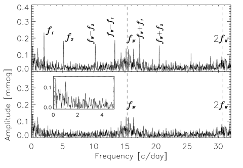
Figure 4: The amplitude spectrum of the wire light curve of $\psi$ Cen is shown in the top panel. Two significant peaks at $f_{1}$ and $f_{2}$ are found. The aliases and the wire orbital frequency are marked. The bottom panel is the amplitude spectrum after subtracting these two modes. The inset shows the details at low frequencies; note the change in scale on the ordinate.

5.1 Interpretation of $f_{1}$ and $f_{2}$

The two detected peaks in the amplitude spectrum correspond to periods of about 0.5 and 0.2 days. These periods could be present in the data due to modulation caused by the rotation period of the stars. To examine this possibility we must estimate the absolute radii of the component stars. To convert our accurate relative radii into absolute radii we estimate the semi-major axis from Kepler’s third law with the orbital period and the mass estimates given in Sect. 4. The result is $3.7\pm 0.2$ $R_{\odot}$ for the primary and $1.8\pm 0.1$ $R_{\odot}$ for the secondary.

We use $\,v\sin i$ $=125\pm 15$ km s^-1 for both the primary and secondary component to find rotational periods of $1.49\pm 0.26$ and $0.74\pm 0.13$ days, respectively. To reach a period as low as 0.5 days the secondary star (with $R/R_{\odot}=1.8$) would need to rotate with $v\sin i\simeq 180$ km s^-1. At present we cannot entirely rule this out, since the spectroscopically determined rotational velocity is dominated by the light from the primary.

To conclude, it seems difficult to explain the observed peaks in the amplitude spectrum as due to the rotation of the primary and possibly also the secondary.

An alternate explanation is that the variation is caused by high order low degree $g$-mode oscillations in the primary star. The instability strip predicting the excitation of modes in slowly pulsating B-type stars (SPB) was calculated for solar metallicity by Pamyatnykh (pamyat1999 (1999)). However, we have $T_{\rm eff}$ $=10,450\pm 300$ K for the primary and this is on the cool side of the theoretical SPB instability strip.

C. Aerts (private communication) kindly computed an evolution model for $M/M_{\odot}=3.1$ using the new solar composition (Asplund et al. (2004)) with the clés code. The pulsation code mad was used to test the mode excitation (see, e.g.  Dupret et al. (2003) for more information on these codes). None of the modes were found to be excited for this model for $T_{\rm eff}$ in the interval $10\,450\pm 300$ K. Ignoring this fact we compared the location of the two modes $f_{1}$ and $f_{2}$ to see if we could find a matching evolutionary state for modes with angular degree $l=1$ or $2$.

The modes in the pulsation model are closely spaced around the low frequency mode $f_{1}$ and we cannot find an unambiguous fit. In the frequency range around $f_{2}$ the modes in the model are well separated but both $l=1$ and 2 are possible. For $l=1$ there is a match of observed and computed frequencies at $T_{\rm eff}$ $=10\,250$ K and for $l=2$ both $T_{\rm eff}$ $=10\,200$ K and $10\,600$ K are possible. However we must remember that these estimates are for solar metallicity while the metallicity of $\psi$ Cen is unknown. Accurate temperatures can be found once photometry of the eclipses in multiple filters has been collected and so a definite mode identification should be possible. Also, when the radial velocity curve of $\psi$ Cen is acquired the masses should be constrained to better than 1% and a detailed modelling of this system can be done. This should enable us to probe the extent of core overshoot in the component stars.

It is important to note that the model code does not take rotation into account. Aerts & Kolenberg (2005) used the same evolution code to interpret observations of the photometric variations seen in the main sequence SPB star HD 121190 which is about 1 500 K hotter than $\psi$ Cen. They stress that significant frequency shifts are expected for even moderately rotating stars due to the Coriolis force perturbing the global oscillation modes when the mode frequency is higher than half the rotation frequency. This is indeed the case for both modes seen in $\psi$ Cen. From the estimate made above we find $\Omega_{\rm rot}=1/P_{\rm rot}=0.67\pm 0.12$ c/day for the primary star when assuming $i_{\rm rot}\simeq i_{\rm orbit}=89.0^{\circ}$.

Since current models do not predict oscillations at the $T_{\rm eff}$ of the primary star in $\psi$ Cen another interesting possibility for the excitation could be tidally induced modes. Willems & Aerts (2002) investigated this and found that in relatively close binary systems with highly eccentric orbits it is possible for $l=2$ and $|m|=2$ modes to occur. For this mechanism to work the pulsation frequency in the co-rotating frame must be an integer multiple of the binary orbital frequency. $\psi$ Cen has a long period and so the orbital frequency is low, $f_{\rm orbit}\simeq 0.026$ c/day. Hence, tidal interaction is most likely not the excitation mechanism in this system. Another explanation for the observed modes is excitation of retrograde mixed modes as suggested by Townsend (2005). To explore these possibilities further would require detailed modelling of the $\psi$ Cen system, which is beyond the scope of the current study.

We should mention that wire data are available for the somewhat hotter star $\iota$ Ophiuchus (HD 152614). The spectral type is B8V and we find $T_{\rm eff}$ $=12\,000$ K from Strömgren photometry using the calibration by Napiwotzki et al. (1993). This star is within the SPB instability strip predicted by Pamyatnykh (pamyat1999 (1999)). The amplitude spectrum shows at least four significant modes at 0.82, 2.0, 4.6 and 4.9 c/day. The amplitudes are 0.5 mmag for the low frequency mode and $\simeq 0.2$ mmag for the remaining three modes. Thus, the frequency range and amplitudes are similar to $\psi$ Cen. We obtained a clés model for this star but the mad oscillation code does not predict any modes above 1.5 c/day to be excited for angular degrees $l=1$ and $2$.

Lastly, we see from Fig 4 that in the range of $\delta$ Scuti star variation with periods of $\simeq$1–2 hours (i.e. frequencies from 12–24 c/day) no significant peaks are present with amplitudes above 0.1 mmag. In the region 14–17 c/day this claim is not valid due to the increased noise level from the aliasing. From the light curve solution we have $L_{B}/L_{A}\simeq 0.163$ and so no $\delta$ Scuti pulsation with amplitudes above $\simeq 0.6$ mmag is present in the secondary component.

6 Conclusions

We report the discovery that $\psi$ Cen is a bright detached eclipsing binary. Photometry from the star tracker on the wire satellite shows that the orbit is eccentric and the period longer than about a month. With the photometry from the smei camera we have been able to determine the period of the system to be 38.81252(29) d.

We have fitted the wire and smei light curves using ebop to find precise photometric parameters for $\psi$ Cen. Monte Carlo simulations show that the random error in the fractional radii of the stars is about 0.1%. We have attempted to assess the systematic uncertainties in this modelling by obtaining solutions with the wink and Wilson-Devinney codes as well as with ebop, but have so far been unsuccessful. Experiments have shown that this is probably due to convergence problems with the differential correction algorithms in the comparison light curve codes. We have been able to find that the systematic uncertainty in the radii are at most 0.3%, and a more accurate assessment can be made once the comparison light curve codes have been modified to use a different optimisation algorithm.

Only a very limited number of radial velocity measurements for $\psi$ Cen are available in the literature, and are severely affected by line blending, so new high-resolution spectroscopy will be acquired by our group. With this data we will be able to measure the absolute masses and radii of the component stars of $\psi$ Cen with high accuracy, which should allow us to place strong constraints on the predictions of theoretical stellar models for masses around 2–3$\,{\rm M}_{\odot}$. This will be helped if we are able to determine a precise metal abundance from the spectra of $\psi$ Cen, but the high rotational velocity of the primary component may make this difficult.

We found two significant peaks in the amplitude spectrum at 2.0 and 5.1 c/day with amplitudes of only 0.2 mmag. These frequencies are too high to be due to rotational modulation. We tentatively interpret them as low amplitude $g$-mode oscillations in the primary star. A preliminary comparison with pulsation models shows that a mode identification should be possible once $T_{\rm eff}$ and the mass of primary is in hand. Thus, $\psi$ Cen will be an interesting object both as a classical detached eclipsing binary system and as an object for a detailed asteroseismic study. It is very interesting that our results indicate that the region of SPB stars as determined from theory (Pamyatnykh pamyat1999 (1999)) may have to be extended towards the blue edge of the Cepheid instability strip for main sequence stars. For further discussion of this point we refer to Aerts & Kolenberg (2005).