Monte Carlo radiative transfer in protoplanetary disks

Abstract

Aims. We present a new continuum 3D radiative transfer code, MCFOST, based on a Monte-Carlo method. MCFOST can be used to calculate (i) monochromatic images in scattered light and/or thermal emission, (ii) polarisation maps, (iii) interferometric visibilities, (iv) spectral energy distributions and (v) dust temperature distributions of protoplanetary disks.

Methods. Several improvements to the standard Monte Carlo method are implemented in MCFOST to increase efficiency and reduce convergence time, including wavelength distribution adjustments, mean intensity calculations and an adaptive sampling of the radiation field. The reliability and efficiency of the code are tested against a previously defined benchmark, using a 2D disk configuration. No significant difference (no more than 10%, and generally much less) is found between the temperatures and SEDs calculated by MCFOST and by other codes included in the benchmark.

Results. A study of the lowest disk mass detectable by Spitzer, around young stars, is presented and the colours of “representative” parametric disks are compared to recent IRAC and MIPS Spitzer colours of solar-like young stars located in nearby star forming regions.

1 Introduction

Signatures for the presence of dust are found nearly everywhere in astrophysics. In the context of star and planet formation, dust is abundant in molecular clouds and in the circumstellar environments of a large fraction of stellar objects in the early stages of their evolution. In the circumstellar disks encircling these young stars, where planets are thought to form, the interplay between dust and gas is of paramount importance.

At short wavelengths, dust grains efficiently absorb, scatter, and polarise the starlight. How much radiation is scattered and absorbed is a function of both the geometry of the disk and the properties of the dust. In turns, the amount of absorbed radiation sets the temperature of the dust (and gas) and defines the amount of radiation that is re-emitted at longer, thermal, wavelengths.

The last decade has witnessed the improvement of imaging capabilities with the advent of potent instruments in the optical and near-infrared, and large millimeter interferometers, providing detailed views of the disks around young stars. The sensitivity and wavelength range covered by new instruments is increasing steadily and the mid- and far-infrared ranges are now being explored efficiently by the Spitzer Space Telescope, and new facilities like Herschel and ALMA will soon complete the coverage.

With this unprecedented wealth of data, from optical to radio, fine studies of the dust content and evolution of disks become possible and powerful radiative transfer (RT) codes are needed to fully exploit the data. In this paper we describe such a code, MCFOST.

That code was used extensively to produce synthetic images of the scattered light from disks around young stars. Examples include the circumbinary ring of GG Tau (McCabe et al. 2002; Duchêne et al. 2004), the large silhouette disk associated with IRAS 04158+2805 (Ménard et al. 2006), and an analysis of the circular polarisation in GSS 30 (Chrysostomou et al. 1997).

In §2 below, we briefly describe MCFOST. In section §3, tests and validation of MCFOST are presented. Two examples of applications are presented in §4. Firstly, a study is presented of the minimum mass of disks detectable by Spitzer around young solar-like stars, young low-mass stars, and young brown dwarfs. Secondly, the colours of parametric disks are compared to the Spitzer colours, for both IRAC and MIPS, of samples of T Tauri stars located in nearby star forming regions.

2 Description of the numerical code

MCFOST is a 3D continuum radiative transfer code based on the Monte-Carlo method. It was originally developed by Ménard (1989) to model the scattered light in dense dusty media (including linear and circular polarisations). In this paper, we present an extended version of the original code that includes dust heating and continuum thermal re-emission.

2.1 Geometry of the computation grid

MCFOST uses a spatial grid that is defined in cylindrical coordinates, well adapted to the geometry of circumstellar disks. $N_{r}$ logarithmically-spaced radial grid cells and $N_{z}$ linearly-spaced vertical grid cells are used. The size of the vertical cells follows the flaring of the disk, with a cutoff at 10 times the scale height for each radius. MCFOST allows for the density distribution to be defined arbitrarily, in 3 dimensions, with the limitation that within each cell, quantities are held constant. The density distribution of the media under consideration can be described either by using a parametric model (as in § 3.1) or by including any ad hoc density table, calculated by other means. In the following, the term “local” refers to the properties of a single cell.

2.2 Position-dependent dust distributions

An explicit spatial dependence of the size (and/or composition) distribution $f(a,\@vec{r})$ is implemented in MCFOST. The dust properties are therefore defined locally, i.e., each cell of the disk may contain its own independent dust population. This allows for example to model dust settling towards the disk midplane, variations of the chemical composition of the dust, and/or an increase of ice mantles from the inner, hot regions to the outer, cold edge of the disk.

2.3 Optical dust properties

The dust optical properties are currently computed with the Mie theory, i.e., grains are spherical and homogeneous. The optical properties at a given position in the disk are derived in accordance with the local size and composition distributions $f(a,\@vec{r})$. The extinction and scattering opacities are given by

$$\kappa^{\mathrm{ext/sca}}(\lambda,\@vec{r})=\int_{a_{\mathrm{min}}}^{a_{\mathrm{max}}}\pi a^{2}Q_{\mathrm{ext/sca}}(\lambda,a)f(a,\@vec{r})\,\mathrm{d}a$$ (1)

where $Q_{\mathrm{sca}}(\lambda,a)$ and $Q_{\mathrm{ext}}(\lambda,a)$ are respectively the scattering and extinction cross sections of a grain of size $a$ at a wavelength $\lambda$.

2.4 The radiative transfer scheme in MCFOST

The Monte Carlo method allows to follow individual monochromatic “photon packets” that propagate through the circumstellar environment until they exit the computation grid. The propagation process is governed by scattering, absorption and re-emission events that are controlled by the optical properties of the medium (opacity, albedo, scattering phase function, etc…) and by the temperature distribution. Upon leaving the circumstellar environment, “photon packets” are used to build an SED and/or synthetic images, one image per wavelength.

2.4.1 The emission of “photon packets”

In MCFOST, two general radiation sources are considered : photospheric emission and circumstellar dust thermal emission.

Any number of stars can be considered, at any position in the calculation grid. The photospheric emission can be represented by (i) a sphere radiating uniformly or (ii) a limb-darkened sphere or (iii) a point-like source, whichever is relevant for the problem under consideration. The spectrum of photospheric photons can follow a blackbody or any observed or calculated spectrum. Hot and/or cold spots can be added to the photospheres.

For the dust thermal emission, the density, temperature and opacities are considered constant within each grid cell. Thermal photons emission locations are uniformly distributed within each cell and the emission is assumed to be isotropic.

2.4.2 Distance between interactions

It is natural within a Monte Carlo scheme to estimate the distance a photon packet “travels” between two interactions by means of optical depth (directly related to the density) rather than by physical, linear distance. From a site of interaction, i.e., scattering and emission, the optical depth $\tau$ to the next site is randomly chosen following the probability distribution $p(\tau)=\exp(-\tau)$.

The distance $l$ is computed by integrating the infinitesimal optical depth $\kappa^{\mathrm{ext}}(\lambda,\@vec{r})\rho(\@vec{r})\,\mathrm{d}s$ until the following equality is verified :

$$\tau_{\lambda}=\int_{0}^{l}\kappa^{\mathrm{ext}}(\lambda,\@vec{r})\rho(\@vec{r})\,\mathrm{d}s\leavevmode\nobreak\ .$$ (2)

Once the position of interaction $\@vec{r}$ is determined, the probability that the interaction is a scattering event rather than an absorption event is estimated with the local albedo :

$${p_{\mathrm{sca}}=\mathcal{A}(\lambda,\@vec{r})=\frac{\int_{a_{\mathrm{min}}}^{a_{\mathrm{max}}}\pi a^{2}Q_{\mathrm{sca}}(\lambda,a)f(a,\@vec{r})\,\mathrm{d}a}{\int_{a_{\mathrm{min}}}^{a_{\mathrm{max}}}\pi a^{2}Q_{\mathrm{ext}}(\lambda,a)f(a,\@vec{r})\,\mathrm{d}a}}\leavevmode\nobreak\ .$$ (3)

2.4.3 Scattering

MCFOST includes a complete treatment of linear and circular polarisations by using the Stokes formalism. The state of a light packet is described by its Stokes vector, with $I$ representing the intensity, $Q$ and $U$ the linear polarisation, and $V$ the circular polarisation. The interaction of a photon with a dust particle is described by a $4\times 4$ matrix, the Mueller matrix, ${\bf S}$, also known as the scattering matrix. Since the matrix is defined with respect to the scattering plane, appropriate rotation matrices are required to transform the Stokes parameters between multiple scattering events. In the simplifying case of Mie scattering , the matrix becomes block-diagonal with only 4 different non-zero elements, see Eq. 4.

$$\left(\begin{array}[]{r}I\\ Q\\ U\\ V\\ \end{array}\right)_{i+1}=\left(\begin{array}[]{rrrr}S_{11}&S_{12}&0&0\\ S_{12}&S_{11}&0&0\\ 0&0&S_{33}&S_{34}\\ 0&0&-S_{34}&S_{33}\\ \end{array}\right)\left(\begin{array}[]{r}I\\ Q\\ U\\ V\\ \end{array}\right)_{i}$$ (4)

The direction of scattering is defined by two angles, the scattering angle $\theta$ and the azimuth angle $\phi$ in spherical coordinates. Each individual element $S_{ij}$ of the matrix is a function of the scattering angle and of the wavelength, $S_{ij}=S_{ij}(\theta,\lambda)$. The scattering angle $\theta$ is randomly chosen from the pretabulated cumulative distribution function :

$$F(\theta)=\frac{\int_{0}^{\theta}S_{11}(\theta^{\prime})\,\sin\theta^{\prime}\mathrm{d}\theta^{\prime}}{\int_{0}^{\pi}S_{11}(\theta^{\prime})\,\sin\theta^{\prime}\mathrm{d}\theta^{\prime}}.$$ (5)

For linearly unpolarised incoming light packets, i.e., $Q,U=0$, the distribution of azimuthal angle $\phi$ is isotropic. For light packets with a non-zero linear polarisation, $P=\sqrt{Q^{2}+U^{2}}/I$, the azimuthal angle is defined relative to its direction of polarisation and determined by means of the following cumulative distribution function :

$$F_{\theta}(\phi)=\frac{1}{2\pi}\left(\phi-\frac{S_{11}(\theta)-S_{12}(\theta)}{S_{11}(\theta)+S_{12}(\theta)}\,P\,\frac{\sin(2\phi)}{2}\right)$$ (6)

where $\theta$ was previously chosen from Eq. 5 (Šolc 1989).

The Mueller matrix used in Eqs. 4, 5, and 6 can be defined in two different ways : one Mueller matrix per grain size or one mean Mueller matrix per grid cell. In the latter case, the local Mueller matrix $S(\lambda,\@vec{r})$ is defined by :

$${\bf S}(\lambda,\@vec{r})=\int_{a_{\mathrm{min}}}^{a_{\mathrm{max}}}{\bf S}(\lambda,a)f(a,\@vec{r})\,\mathrm{d}a$$ (7)

where $S(\lambda,a)$ is the Mueller matrix of a grain of size $a$ at a wavelength $\lambda$.

In the former case, the grain size must be chosen explicitly for each event following the probability law :

$$p(a)\mathrm{d}a=\frac{\pi a^{2}Q_{\mathrm{sca}}(a)f(a,\@vec{r})\,\mathrm{d}a}{\int_{a_{\mathrm{min}}}^{a_{\mathrm{max}}}\pi a^{2}Q_{\mathrm{sca}}(a)f(a,\@vec{r})\,\mathrm{d}a}\leavevmode\nobreak\ .$$ (8)

The two methods are strictly equivalent. They can be used alternatively to minimize either the memory space or the computation time required.

2.4.4 Absorption and radiative equilibrium

The temperature of the dust particles is determined by assuming radiative equilibrium in the whole model volume, and by assuming that the dust opacities do not depend on temperature.

The dust thermal balance should take into account the thermal coupling between gas and dust. In high density regions, e.g., close to the disk midplane, the coupling is very good and the gas temperature is expected to be close to the dust temperature. At the surface layers of the disk, on the other hand, densities become much lower and gas-dust thermal exchanges are reduced.

Two extreme assumptions are implemented in MCFOST : either the gas-dust thermal exchange is perfect and gas and dust are in local thermodynamic equilibrium (LTE) throughout the disk, or there is no thermal coupling between gas and dust at all. In the latter case, each grain size has its own, different temperature, despite being in equilibrium with the same radiation field.

Under the assumption of LTE, all dust grains have the same temperature, which is also equal to the gas temperature. In this case, the (unique) temperature of the cell is given by the radiative equilibrium equation :

$$4\pi\int_{0}^{\infty}\kappa_{i}^{\mathrm{abs}}(\lambda)B_{\lambda}(T_{i})\,\mathrm{d}\lambda=\Gamma_{i}^{\mathrm{abs}}$$ (9)

where $\Gamma_{i}^{\mathrm{abs}}$ is the energy absorption rate. If only passive heating is considered, this rate can be written from the mean intensity, leading to :

$$4\pi\int_{0}^{\infty}\kappa_{i}^{\mathrm{abs}}(\lambda)B_{\lambda}(T_{i})\,\mathrm{d}\lambda=4\pi\int_{0}^{\infty}\kappa_{i}^{\mathrm{abs}}(\lambda)J_{\lambda}\,\mathrm{d}\lambda.$$ (10)

Any extra internal source of energy (viscous heating for instance) can be easily included by adding the corresponding term on the right hand side of Eq. 10.

Each time a packet $\gamma$ of a given wavelength $\lambda$ travels through a cell, the quantity $\Delta l_{\gamma}$, the distance travelled by the packet in the cell, is computed. The mean intensity $J_{\lambda}$ in the cell is then derived following Lucy (1999):

$$J_{\lambda}=\frac{1}{4\pi V_{i}}\sum_{\gamma}\varepsilon\,\Delta l_{\gamma}=\frac{1}{4\pi V_{i}}\sum_{\gamma}\frac{L_{*}}{N_{\gamma}}\,\Delta l_{\gamma}$$ (11)

where $V_{i}$ is the volume of cell $i$ and $\varepsilon$ the individual luminosity of a packet. The radiative equilibrium equation can then be written as :

$$\int_{0}^{\infty}\kappa_{i}^{\mathrm{abs}}(\lambda)B_{\lambda}(T_{i})\,\mathrm{d}\lambda=\frac{L_{*}}{4\pi V_{i}N_{\gamma}}\sum_{\lambda,\gamma}\kappa_{i}^{\mathrm{abs}}(\lambda)\Delta l_{\gamma}\leavevmode\nobreak\ .$$ (12)

This method is known as the mean intensity method.

When gas and dust, as well as dust grains of different sizes, are not thermally coupled, there is a different temperature for each grain size and the radiative equilibrium must be written independently for each of them :

$$4\pi\int_{0}^{\infty}\kappa_{i}^{\mathrm{abs}}(\lambda,a)B_{\lambda}(T_{i}(a))\,\mathrm{d}\lambda=\Gamma_{i}^{\mathrm{abs}}(a)$$ (13)

where $\kappa_{i}^{\mathrm{abs}}(\lambda,a)$, $T_{i}(a)$ and $\Gamma_{i}^{\mathrm{abs}}(a)$ are the opacity, temperature and energy absorption rate of the dust grains of size $a$ in cell $i$.

The calculation of $\int_{0}^{\infty}\kappa_{i}^{\mathrm{abs}}(\lambda)B_{\lambda}(T_{i})\,\mathrm{d}\lambda=\sigma T^{4}\kappa_{P}/\pi$ ($\kappa_{P}$ is the Planck mean opacity) is very time consuming and we pretabulate these values at $N_{T}=1\,000$ logarithmically spaced temperatures ranging from $1$K to the sublimation temperature, which is of order $1\,500$ K. The temperature $T_{i}$ of each cell is obtained by interpolation between the pretabulated temperatures.

To speed up calculations, Bjorkman & Wood (2001) introduced the concepts of immediate reemission and temperature correction. They are implemented in MCFOST. In essence, when a packet is absorbed, it is immediately re-emitted and its wavelength chosen by taking into account the temperature correction given by the following probability distribution :

$$p_{\lambda}\,\mathrm{d}\lambda\propto\kappa_{\mathrm{i}}^{\mathrm{abs}}(\lambda)\left(\frac{\mathrm{d}B_{\lambda}}{\mathrm{d}T}\right)_{T_{i}}\,\mathrm{d}\lambda\leavevmode\nobreak\ .$$ (14)

Baes et al. (2005) suggested that this wavelength distribution adjustment method may not be entirely safe when used in combination with the mean intensity writing of the absorption rate described above. Instead, MCFOST determines the cell temperatures $T_{i}$ used in Eq. 14 by solving :

$$\int_{0}^{\infty}\kappa_{i}^{\mathrm{abs}}(\lambda)B_{\lambda}(T_{i})\,\mathrm{d}\lambda=\frac{L_{*}}{4\pi V_{i}N_{\gamma}}N_{\gamma\ \mathrm{abs},i}$$ (15)

where $N_{\gamma\ \mathrm{abs}}$ is the current number of absorbed photons in cell $i$. Eq. 12 is used only at the end, when all photons have been propagated, to improve the accuracy of the temperature determination. Using Eq. 15 instead of Eq. 12 when computing temperature for Eq. 14 is in no way a limitation because, at this stage of the computation, the aim is to compute the radiation field and not the whole temperature structure. Of course, the temperature in optically thin cells will not be precisely determined because little absorption occurs in these cells. On the other hand, as a consequence, little reemission will also occur and the contribution of these reemission events will remain very small. By construction of the Bjorkman & Wood (2001) method, temperature is best converged in the cells that contribute most to the radiation field. So, when all photons have been propagated, temperature corrections are no longer needed and the temperature of all cells can be computed following the Lucy (1999) method, providing a much higher final accuracy.

2.4.5 SED calculation: sampling of the radiation field

To improve its computational efficiency when producing SEDs, MCFOST uses different samplings of the radiation field, i.e., different strategies to set the energy of a photon packet. The energy of a packet, hence the number of photons it contains, is chosen and optimised depending on the goals of the calculation. On the one hand, the convergence of the temperature distribution is optimized when all photon packets have the same energy, independently of their wavelengths. This procedure insures that more photon packets are emitted in the more luminous bins. On the other hand, the computation of SEDs itself is more efficient when it is the number of photon packets that is held constant for all wavelength bins instead. In that case it is the energy of the packets that is wavelength dependent. Thus, MCFOST is made more efficient by computing the temperature and SEDs with a two-step process:

• Step 1 is the temperature determination. Photon packets are generated and calculated one by one at the stellar photosphere and propagated until they exit the computation grid, i.e., until they exit the circumstellar medium. Upon scattering, the propagation vector of a packet is modified, but not its wavelength. Upon absorption however, packets are immediately re-emitted, in situ and isotropically, but at a different wavelength calculated according to the temperature of the grid cell. For this re-emission process, the concept of immediate reemission and the associated temperature correction method proposed by Bjorkman & Wood (2001) are used. In this step, all photon packets have the same luminosity

  $$\epsilon=L_{*}/N_{\gamma step1}$$ (16)

  where $L_{*}$ is the bolometric luminosity of the star and $N_{\gamma step1}$ the number of packets generated, and are randomly scattered/absorbed within the disk. The concept of mean intensity suggested by Lucy (1999) is further used to compute the final temperature at the end of the step. This allows to efficiently reduce noise in the temperature estimation for optically thin cases. Step 1 allows for a fast convergence of the temperature but is rather time-consuming when used to derive SEDs, especially in the low-energy, long wavelength regime. To speed up convergence, a different scheme (step) is used to compute SEDs.

• Step 2 computes the SED from the final temperature distribution calculated in step 1. In step 2, the number of photon packets $N_{\gamma step2}$ is held constant at all wavelengths. Step 2 therefore maintains a comparable noise level in each wavelength bins and significantly reduces convergence time by limiting the CPU time spent in high luminosity bins and focusing on low luminosity bins. In this step, photon packets are always scattered, no absorption is allowed. However, at each interaction, the Stokes vector is weighted by the probability of scattering, $p_{\mathrm{sca}}$, to take into account the energy that would have been removed by absorption. This allows all the photons to exit the disk and to contribute to the SED, although with a reduced weight. Packets at a given wavelength $\lambda$ are randomly emitted from the star and the disk, by cells $i$, with the respective probabilities :

  $$p_{*}=\frac{L_{*}(\lambda)}{L_{*}(\lambda)\leavevmode\nobreak\ +\leavevmode\nobreak\ \sum_{i}\leavevmode\nobreak\ w_{i}(\lambda)\,L_{i}(\lambda)}\leavevmode\nobreak\ ,$$ (17)

  $${\rm and}\leavevmode\nobreak\ p_{i}=\frac{w_{i}(\lambda)\,L_{i}(\lambda)}{L_{*}(\lambda)\leavevmode\nobreak\ +\leavevmode\nobreak\ \sum_{i}\leavevmode\nobreak\ w_{i}(\lambda)\,L_{i}(\lambda)}\leavevmode\nobreak\ .$$ (18)

  where the luminosities are defined by :

  $$L_{*}(\lambda)=4\pi^{2}R_{*}^{2}\,B_{\lambda}(T_{*})\leavevmode\nobreak\ ,$$ (19)

  $${\rm and}\leavevmode\nobreak\ L_{i}(\lambda)=4\pi\,m_{i}\,\kappa_{i}^{\mathrm{abs}}(\lambda)\,B_{\lambda}(T_{i})\leavevmode\nobreak\ .$$ (20)

  In order to avoid generating photon packets so deep in the (very optically thick) disk that none of them would escape with an appreciable energy left, a “dark zone” is defined for each wavelength. This dark zone includes all cells from which the optical depth is at least $\tau_{\lambda}=30$, in any direction, to get out of the computationnal grid. No photon packet is emitted from this zone, the emission probability from cells inside the dark zone being set to zero by fixing a weight $w_{i}(\lambda)=0$. A weight $w_{i}(\lambda)=1$ is given to cells above the dark zone limit. Furthermore, packets that would enter the dark zone during their random walk are killed, because they have no chance to exit the model volume with significant energy. The luminosity of the $N_{\gamma step2}$ packets emitted at a given wavelength $\lambda$ is determined by the total energy that the star and the disk radiates at this wavelength :

  $$\epsilon_{\lambda}=\frac{L_{*}(\lambda)\leavevmode\nobreak\ +\leavevmode\nobreak\ \sum_{i}\leavevmode\nobreak\ w_{i}(\lambda)\,L_{i}(\lambda)}{N_{\gamma step2}}\leavevmode\nobreak\ .$$ (21)

2.4.6 Intensity and polarisation maps

A scheme similar to step 2 used above to calculate SEDs is deployed in MCFOST to calculate synthetic maps. Maps are calculated, one wavelength at a time. Scattering is treated explicitly for all wavelengths but again, absorption is replaced by the appropriate weighting of the intensity to avoid losses of photon packets. Images are produced, in all four Stokes parameters, by classifying photon packets that exit the calculation grid into inclination bins, themselves divided into image pixels. The same process applies to scattered light images in the optical and thermal emission maps in the far infrared and radio range. The relative contribution of the photospheric and dust thermal emission is dependent on the wavelength. It is for instance critical in the mid-infrared and beyond where it is the (scattered) thermal emission from the inner disk that starts to dominate over the photospheric contribution. The correct fraction is calculated explicitly through the temperature and density of each disk cell and each contribution can be mapped separately for comparison. Interferometric visibilities and phases can be obtained by Fourier transform of images.

Figure 1: Plots of the radial temperature (upper panel) and the difference (lower panel) for the most optically thick case, $\tau_{\mathrm{V}}=100$, arbitrarily using RADICAL as the reference. In both panels, the results of MCFOST are represented by the thick solid line. Thin solid lines are the results from MC3D, dot-dashed lines from MCTRANSF, dotted lines from RADMC and dashed lines from STEINRAY. In the upper panel, because all curves are very similar, MCFOST has been shifted by 200K for clarity.

3 Tests and validation of MCFOST

Numerous tests have been performed to check the efficiency, stability, and accuracy of MCFOST. In this section, we present a comparison of MCFOST with the benchmark results published by Pascucci et al. (2004) (hereafter P04).

Figure 2: Plots of the difference between the model SEDs for the most optically thick case, $\tau_{\mathrm{V}}=100$, arbitrarily using RADICAL as the reference code. The linestyle-to-code pairing is the same as in Fig. 1. Three different inclination angles are considered: $i=12.5^{\circ}$ (upper panel), $i=42.5^{\circ}$ (middle panel), and $i=77.5^{\circ}$ (lower panel).

3.1 Benchmark definition

The geometry tested involves a central point-like source radiating as a T=$5\,800$K blackbody with a bolometric luminosity $L=L_{\odot}$ encircled by a disk of well defined geometry and dust content. The disk extends from 1 AU to 1 000 AU. It includes spherical dust grains made of astronomical silicate. Grains have a single size radius of $0.12\ \mu$m and a density of $3.6\ \mathrm{g.cm}^{-3}$. The optical data are taken from Draine & Lee (1984). The disk is flared with a Gaussian vertical profile. Radial power-law distributions are used for the surface density and the scale height (see P04 for more details).

To compare with P04, the scattering is also forced to be isotropic and polarisation is not calculated, i.e, all the scattering information is contained in the scattering cross section alone, $Q_{sca}$, acting on the I Stokes parameter only.

The number of grid cells is set to $N_{r}=50$ and $N_{z}=20$ in the radial and vertical directions, respectively. We used $10^{7}$ photon packets to calculate the temperature distribution (step 1) and $2\,10^{6}$ photon packets per wavelength to generate the SED (step 2). The total run-time is $20$ minutes for the most optically thick case on a bi-processor (Intel Xeon) computer running at a clock rate of 2.4 GHz. The run-time memory space needed is $10$ MBytes.

3.2 Results

The results calculated with MCFOST for all the test cases presented in P04 are available at http://www-laog.obs.ujf-grenoble.fr/~cpinte/mcfost/. Only the most optically thick case ($\tau_{\mathrm{V}}=100$, see P04), i.e., the most difficult one, is presented in Figs. 1 and 2.

The temperature profiles in the disk and shape of the emerging SEDs calculated with MCFOST are in excellent agreement with the calculation presented in P04. Differences in the radial temperatures computed by MCFOST do not exceed 4% with respect to the other 5 codes in the optically thin case. For the most optically thick case, differences are generally of the order of 2-5% (see Fig. 1). The results from MCFOST are always within the range of those produced by other codes.

Regarding SEDs, MCFOST produces results comparable to all other codes to better than 10% for low optical thickness. Deviations as large as 15% are however observed in the most defavorable case, i.e., high tilt and optical thickness (either at very short wavelength or in the 10 $\mu$m silicate feature), but again the results lie in the range of the values produced by other codes (see Fig. 2).

Various tests were further performed to show the independence of the MCFOST results with respect to grid sampling, inclination sampling, and position of the vertical density cut-off in the disk. Results are not noticeably affected. A complete description of all numerical tests is presented in Pinte et al. (2005).

3.3 Energy conservation at high optical depth

As discussed in section 2.4.5, SEDs can be constructed from packets escaping the system in both steps of the computation (the SED from step 2 being better converged by construction). As photon packets are generated independently through different processes in step 1 and 2, our adaptive sampling of the radiation field method allows an a posteriori check of the accuracy of calculations.

By integrating over all inclination angles and wavelengths, the emerging flux must correspond in both cases to the star luminosity (in case of passive heating). This is true by construction for the SED calculated in step 1.

Assuming a standard flared disk geometry and ISM like grains, and varying (via the disk mass) the V band equatorial optical depth from $0.1$ to $10^{9}$, we find that the luminosities calculated through the 2 methods always agree to within better than $1\%$.

4 Example of applications of MCFOST

In this section we present calculations of the SEDs and infrared photometric colours of young objects surrounded by circumstellar disks. The colours calculated by MCFOST are compared with photometric observations obtained with the Spitzer Space Telescope. Calculated infrared fluxes as a function of disk mass are also compared with Spitzer’s detection limits, as obtained for example during legacy surveys like c2d (Evans et al. 2003). The goals are (i) to explore whether a disk with “representative” geometrical parameters can match the observed infrared colours of solar-like young stars and (ii) also to estimate the range of disk masses detectable by Spitzer in such programmes.

4.1 Disk geometry and central object properties

Table 1: Star parameters

Central object	Mass ($M_{\odot}$)	Radius ($R_{\odot}$)	$T_{\mathrm{eff}}$
T Tauri star	1.0	1.94	4 420 K
Low mass star	0.2	1.28	3 365 K
Brown dwarf	0.05	0.57	2 846 K

Figure 3: SEDs for different dust disk masses and central objects, for a pole-on disk. The left panel presents the results for the T Tauri star and $R_{\mathrm{in}}=0.1$ AU, the central panel for the very low mass star and the right panel for the brown dwarf (defined in table 1). The line type corresponds to the disk dust mass (in solar masses). The horizontal bars indicate Spitzer’s detection limits in the four IRAC bands and the $24\ \mu$m and $71\ \mu$m MIPS bands for the molecular cloud mapping programme of the Cores to Disks legacy survey. Additional MIPS limits (light gray bars : $170$ mJy at $24\ \mu$m and $1\,000$ mJy at $71\ \mu$m) for deeper pointed observations of the programme are also plotted at $24\ \mu$m and $71\ \mu$m.

We assume a disk geometry that is representative of the geometries derived from images of several disk sources (HK Tau B : Stapelfeldt et al. 1998 ; HV Tau C : Stapelfeldt et al. 2003 ; IRAS 04158+2805 : Glauser et al. 2006 ; TW Hya : Krist et al. 2000 ; LkHa 263 C : Chauvin et al. 2002). The disk geometry is kept constant through the various model runs but the disk mass is varied. Only disks with dust masses smaller than $10^{-6}M_{\odot}$ are considered in order to focus on the transition between optically thick and optically thin disks, i.e., from class II to class III young stellar objects.

The disk is defined by a flared geometry with a vertical Gaussian profile $\rho(r,z)=\rho_{0}(r)\,\exp(-z^{2}/2\,h(r)^{2})$. Power-law distributions describe the surface density, $\Sigma(r)=\Sigma_{0}\,(r/r_{0})^{\alpha}$, and the scale height, $h(r)=h_{0}\,(r/r_{0})^{\beta}$, where $r$ is the radial coordinate in the equatorial plane, $h_{0}=10$ AU is the scale height at the reference radius $r_{0}=100$ AU, $\beta=1.125$, and $\alpha=-1$. The outer radius is set to $R_{\mathrm{out}}=300$ AU. Two values of the disk inner radius are considered: $0.1$ AU and $1$ AU. A grid of models is calculated from dust disk masses ranging from $10^{-13}$ to $10^{-6}M_{\odot}$. Calculations are presented with masses sampled logarithmically, by steps of $\sqrt{10}$.

A grain size distribution $\mathrm{d}n(a)\propto a^{-3.7}\,\mathrm{d}a$ of spherical particles ranging from $a_{\mathrm{min}}=0.03\ \mu$m to $a_{\mathrm{max}}=1\$mm, and optical constants from Mathis & Whiffen (1989), namely their model A, are used.

The central stars are assumed to emit like blackbodies. Three different central light sources are considered. They are chosen to represent a typical T Tauri star, a low mass star, and a brown dwarf (see Tab. 1 for parameters). The radii and effective temperatures of the T Tauri and low-mass stars are obtained from the models of Siess et al. (2000), assuming an age of $2$ Myrs and a metallicity $Z=0.1$. For the brown dwarf, a mass of $0.05$ M_⊙ is selected. The photospheric properties are taken from Chabrier et al. (2000) and from Baraffe et al. (2002) dusty models. These parameters are summarized in Tab. 1.

All models are calculated for a distance d=140 pc, typical of nearby star forming regions.

4.2 Detectability of disk infrared excesses with Spitzer

In Fig. 3, SEDs are presented as a function of disk dust mass for the three objects to evaluate the minimum detectable disk mass as a function of the luminosity of the central star. For comparison, a set of detection limits reached by Spitzer for large mapping programmes is overplotted. Here we take the values quoted by the Spitzer legacy survey team Cores to Disks for their molecular cloud mapping programme (Evans et al. 2003) .

At all 4 IRAC bands, the photospheric emission is always above the detection limit, for all types of objects. At $24\ \mu$m, the T Tauri and low-mass photospheres are detected. However, the photosphere of the brown dwarf is $\approx 3$ times lower than the detection limit. This is of course dependent on the exact detection limit chosen and on the actual mass of the brown dwarf.

For the case considered here, i.e., detection limits for large mapping programmes and substellar object of 0.05M_⊙, a flux detection at $24\ \mu$m readily implies the presence of circumstellar material. A more careful analysis is required to confirm a disk excess in the case of more massive objects. At $71\ \mu$m, the photosphere is detected for none of the objects and the presence of circumstellar dust can be directly inferred from any detection.

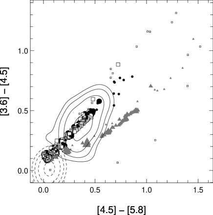
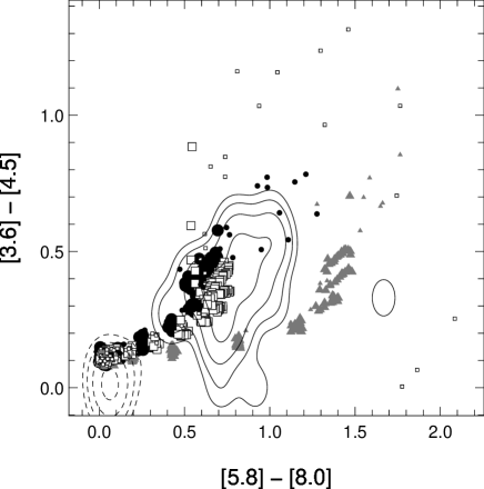
Figure 4: IRAC colour-colour diagrams. Black filled circles corresponds to models with $R_{\mathrm{in}}=0.1$ AU and large grains ($a_{\mathrm{max}}=1$ mm), gray triangles to models with $R_{\mathrm{in}}=1.0$ AU and large grains, white squares to models with $R_{\mathrm{in}}=0.1$ AU, with interstellar dust ($a_{\mathrm{max}}=1\ \mu$m). Large symbols show inclinations smaller than $80^{\circ}$ and small symbols $i>80^{\circ}$. Class II and Class III data points from Hartmann et al. (2005) were converted to surface densities using a Gaussian convolution ($\sigma=0.07$ mag). The solid and dashed contours define the location of class II and class III objects; respectively. The levels are [0.1, 0.2, 0.4, 0.8] of the maximum of density.

Reverting the argument, for an observing programme with such detection limits, Spitzer is expected to detect, at $71\leavevmode\nobreak\ \mu$m, dust disk masses as low as $3\,10^{-9}$ M_⊙ around T Tauri stars, with $R_{\mathrm{in}}=0.1$ AU (Fig. 3, left panel). For low mass stars, disk masses greater than $3\,10^{-8}$ M_⊙ will be detected (Fig. 3, central panel), and for a brown dwarf of 0.05M$\odot$, disk masses larger than $3\,10^{-7}$ M_⊙ are required for detection (Fig. 3, right panel). All results are given in terms of dust mass. A gas-to-dust ratio has to be assumed to extrapolate to total disk masses.

4.3 Spitzer colours

Hartmann et al. (2005) have used Spitzer/IRAC to determine the location of TTS (Class II and III) in colour-colour diagrams. Here we attempt to reproduce the global location of these sources in the colour-colour diagrams. The precise location depends on the model geometry. Similar studies of IRAC colours have been presented elsewhere (D’Alessio et al. 2006). Here, we present the colours of a few parametric models of passive disks to explore the range of parameters that reproduce IRAC colours. We also compare the same model with MIPS colours recently published (Padgett et al. 2006).

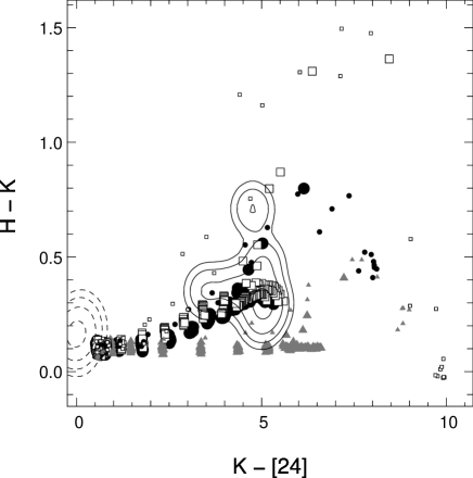
Figure 5: MIPS colour-colour diagram. The symbols are the same as in Fig. 4. The solid and dashed contours define the location of class II and class III from Padgett et al. (2006), respectively. The Gaussian convolution was performed with $\sigma=0.07$ mag along the H - K axis and $\sigma=0.35$ mag along the K -[24] axis.

Fig. 4 and 5 show the modelled IRAC and MIPS colours for the previously defined T Tauri ($1M_{\odot}$) models. Models for central objects with lower masses (not displayed for clarity) presents similar colours and, as a consequence, the comparison of our results for a unique central object mass with the distribution of masses of Hartmann et al. (2005) and Padgett et al. (2006) sources is relevant. Additional models with interstellar dust, where $a_{\mathrm{max}}=1\ \mu$m and larger inner radius $R_{\mathrm{in}}=1$ AU are also presented. Three data sets ( $R_{\mathrm{in}}=0.1$ AU and $a_{\mathrm{max}}=1$ mm ; $R_{\mathrm{in}}=1$ AU and $a_{\mathrm{max}}=1$ mm ; $R_{\mathrm{in}}=0.1$ AU and $a_{\mathrm{max}}=1\ \mu$m) are then displayed, each one calculated for $15$ different disk masses and for $21$ different inclinations, linearly sampled from pole-on to edge-on. Contour plots showing the observed colours of Taurus class II and class III sources (from Hartmann et al. 2005 in Fig. 4 and Padgett et al. 2006 in Fig. 5) are surimposed.

Broadly speaking, models sample the two regions of the colour-colour diagram where sources are found : low disk mass models corresponding to class III objects and higher disk mass models to class II.

The slight offsets seen between the lowest mass models and the class III region is due to the colours of the blackbody spectrum we used. Using a more realistic spectrum would produce, for instance, a [3.6] - [4.5] colour index of $-0.04$ mag instead of $0.1$ mag for the blackbody spectrum, in better agreement with the observations.

For increasing disk masses, all IRAC and MIPS colour indices increase toward the class II region. The models also populate the intermediate region where no object are observed. These results can be used to confirm that the transition between class II (disk dust mass $>3\,10^{-9}$ M_⊙) and class III (disk dust mass $<10^{-10}$) M_⊙ must be fast enough so that no or very few objects are detected in samples of nearly 50 sources (Hartmann et al. 2005).

A clear difference is seen between models depending on the disk inner radius : models with $R_{\mathrm{in}}=1$ AU produce redder [4.5] - [5.8] and [5.8] - [8.0] colours. In particular, with $R_{\mathrm{in}}=1$ AU the [5.8] - [8.0] colour index becomes larger than the observed value by about $0.5$ mag for large masses, suggesting that $R_{\mathrm{in}}=1$ AU is an upper limit for most class II disks in Taurus. This suggestion is supported by the H - K / K - [24] diagram, where no excess is seen in H - K for models with $R_{\mathrm{in}}=1$ AU, well below the average H - K $=0.3$ seen in observations (see gray triangles in Fig. 4 and 5). Such a behaviour is explained by the much higher temperature reached in models with $R_{\mathrm{in}}=0.1$ AU, for which disk emission peaks between $2$ and $3\,\mu$m, whereas it peaks around $10\,\mu$m in models with $R_{\mathrm{in}}=1.0$ AU.

Models close to edge-on ($i>80^{\circ}$) tend to produce redder colour at large masses than their less tilted counterparts. Because the central star becomes more attenuated by its disk, the contribution from the disk emission progressively dominates, leading to rising mid-infrared SEDs. The resulting colours are reminiscent of Class I objects, and highlight the necessity to determine the geometry and inclination, in order to correctly assess the nature of a class I source, i.e., the presence or not of a massive envelope (Kenyon & Hartmann 1995; White & Hillenbrand 2004)

No significant influence of the grains size is detectable for models where the star is seen directly (with $i<80^{\circ}$). At high inclinations, on the contrary, models with interstellar dust produce redder colour indices than models with large grains, for which absorption tends to be gray.

For completely edge-on models, when no direct light from the star reaches the observer, short wavelength colours : [3.6] - [4.5] and H - K strongly depend on scattering properties. Models with interstellar dust present almost no excess at short wavelength, most of the light being scattered starlight. At longer wavelength, direct emission from the disk is seen, producing red indices. For models with larger grains, the albedo remains non negligible in the infrared, and the contribution of thermal emission from the central (and hidden) parts of the disk scattered by the outer parts towards the observer is non negligible and adds to the stellar scattered light, resulting in redder [3.6] - [4.5] and H - K indices than with interstellar dust.

5 Summary

We have presented a new continuum 3D radiative transfer code, MCFOST. The efficiency and reliability of MCFOST was tested considering the benchmark configuration defined by P04. MCFOST was shown to calculate temperature distributions and SEDs that are in excellent agreement with previous results from other codes.

Sets of models for young solar-like stars and low-stars are presented and compared to the Spitzer’s detection limits for the programme of the Cores to Disks legacy survey. Minimal disks masses of $\approx 10^{-9}$ M_⊙ for a T Tauri star and $\approx 10^{-7}$ M_⊙ for a brown dwarf are needed for the disk to be detectable by Spitzer in the mapping mode.

IRAC and MIPS colours of Taurus Class II and III objects are compared to passively heated models with a “representative” disk geometry. The average location of the two classes of objects are well reproduced, as well as the extreme colours of some of the objects, that may correspond to highly tilted disks. $R_{\mathrm{in}}=1$ AU is found to be maximum inner radius required to account for the observed colours of Class II objects. Further modelling of individual sources, combining optical, infrared and millimeter photometry with images and/or IRS spectroscopy, will be needed to better understand individual disks, their dust properties and their evolution.