The Cosmic Microwave Background and the Ionization History of the Universe

Abstract

Details of how the primordial plasma recombined and how the universe later reionized are currently somewhat uncertain. This uncertainty can restrict the accuracy of cosmological parameter measurements from the Cosmic Microwave Background (CMB). More positively, future CMB data can be used to constrain the ionization history using observations. We first discuss how current uncertainties in the recombination history impact parameter constraints, and show how suitable parameterizations can be used to obtain unbiased parameter estimates from future data. Some parameters can be constrained robustly, however there is clear motivation to model recombination more accurately with quantified errors. We then discuss constraints on the ionization fraction binned in redshift during reionization. Perfect CMB polarization data could in principle distinguish different histories that have the same optical depth. We discuss how well the Planck satellite may be able to constrain the ionization history, and show the currently very weak constraints from WMAP three-year data.

1 Introduction

We are entering the era of precision cosmology, with future high precision cosmic microwave background (CMB) data in the offing. If the physics governing the evolution of the photon distribution can be modelled reliably, this data offers an almost unique opportunity to measure a large number of cosmological parameters accurately and distinguish models of the early universe. It is widely recognized that small second (and higher) order effects can effect the CMB power spectra at the several-percent level: these include the kinetic and thermal Sunyaev-Zel’dovich (SZ) effects (Hu & Dodelson, 2002) and CMB lensing (Lewis & Challinor, 2006). As well as the cosmological parameters of most interest, there are however also other uncertain parameters governing the background evolution of the universe that can be of comparable importance.

Here we focus on the ionization history, parameterized as the ionization fraction as a function of redshift. The broad details of recombination are well understood (Peebles, 1968, 1993; Hu et al., 1995). Direct recombination to the ground state is ineffective as it releases a high energy photon that immediately ionizes another atom: it can only be important if the photon is sufficiently cosmologically redshifted before encountering another atom. The dominant mechanism is in fact capture to an excited state followed by a two-photon transition to the ground state. However there are many excited states in both hydrogen and helium, giving many possible recombination channels. Furthermore level populations may be out of equilibrium, requiring a full multi-level atom evolution to calculate the recombination rate accurately (Seager et al., 2000). This can only be done to the extent that the different transition rates are known (or can be calculated), in particular excited state two-photon transition rates are not known very well and are potentially important (Dubrovich & Grachev, 2005). The two-photon rates can also differ significantly from their empty-space value due to induced decay by CMB photons (Chluba & Sunyaev, 2006).

Most current CMB power spectrum calculations use the effective model used in the code recfast (Seager et al., 1999). However the ionization fraction from this code differs by several percent from a more recent calculation in Dubrovich & Grachev (2005) that includes additional transitions. Level splitting and other neglected effects can also have percent-level effects on the CMB power spectra (Chluba & Sunyaev, 2006; Leung et al., 2004; Rubino-Martin et al., 2006). Furthermore there is no full calculation with any quantification of the error. When high resolution CMB data are available we will either need to be able to calculate the recombination history sufficiently accurately that errors can be neglected, or we will need to include uncertainties in any analysis. Not surprisingly assuming an incorrect history can give biased constraints on the cosmological parameters inferred from CMB data (Hu et al., 1995). Our aim in this paper is to see whether a crude parameterization of uncertainties in recombination can be used with future data to give reliable parameter constraints when considerable uncertainties remain in the details of recombination. The detailed task of improving recombination models and parameterizing residual uncertainties is an important challenge for the future.

Once recombination has proceeded to reduce the residual ionized density to a low level the details are no longer important for the CMB: the electron density is so low that few CMB photons are scattered. However at some point first collapsed objects will form, and at some later time high-energy photons emitted by (for example) quasars or stars of various populations can cause the universe to reionize (Loeb & Barkana, 2001; Gnedin & Fan, 2006). Current observations of quasar absorption spectra only put a lower bound on reionization redshift, giving evidence for the first neutral hydrogen on our light cone at $z\approx 6$ (Becker et al., 2001; Fan et al., 2006). Exactly how the ionization fraction evolved between the low level remaining after recombination and $z\approx 6$ is unknown in any detail.

The main CMB constraint on reionization comes from the large scale polarization signal generated by scattering of the CMB quadrupole during reionization. This gives a characteristic bump in the large scale polarization power spectra on scales larger than the horizon size at reionization, and the exact details of the shape of the bump can in principle be used to constrain the ionization history (Kaplinghat et al., 2003; Hu & Holder, 2003). Scales smaller than the horizon size are uniformly damped, leading to a suppression of the acoustic peaks of $e^{-2\tau}$ where $\tau$ is the optical depth to reionization; the small scales cannot therefore be used to constrain the details of the history, only the total optical depth. Beyond linear theory there are also tiny secondary anisotropies on small scales that we do not discuss further here (Weller, 1999; Hu, 2000).

The current constraint on the optical depth from the WMAP three-year polarization observations is $\tau=0.09\pm 0.03$ (Page et al., 2006; Spergel et al., 2006), significantly smaller than $\tau\sim 0.17$ favoured by the one-year data (which had unsubtracted foreground contamination). The new value may be more consistent with simple reionization scenarios, though the lower fluctuation amplitude measured by the three-year data makes this interpretation unclear; for discussion see Alvarez et al. (2006); Popa (2006).

Since there is currently no convincing model of the reionization history we attempt to constrain it in a relatively model independent way. Hu & Holder (2003) suggest a binned fit and performed a principal component analysis with Fisher matrix techniques. They showed that the first two to three eigenmodes should be fairly well constrained with future observations, but other details are effectively unconstrained by the CMB alone. In the second part of this paper we investigate how the reionization history binned in redshift can be constrained with current, perfect, and simulated Planck (Planck, 2006) data. The general constraints we obtain are rather weak, however distinct models of reionization can be distinguished. Unless there is a convincing physical model for how reionization proceeds, flexible modelling of the reionization history is required in order not to obtain biased constraints on the optical depth (and hence the amplitude of primordial fluctuations and $\sigma_{8}$ inferred from the CMB).

Since details of reionization are only important on large scales, and details of recombination are only important on small scales, the two effects are virtually independent. We start by describing our parameter estimation and forecasting methodology, then move on to consider recombination and reionization separately.

2 Parameter estimation and forecasting

We make use of standard Markov Chain Monte Carlo (MCMC) methods to sample from the posterior distribution of the parameters given real or forecast data. Extra parameters governing the ionization history are added to the code camb (Lewis et al., 2000) (based on cmbfast (Seljak & Zaldarriaga, 1996)) for computing the CMB anisotropies. This is then used with a modified version of CosmoMC (Lewis & Bridle, 2002) to generate samples from the posterior distribution.

For idealized forecasting work we assume that the temperature $T$ and polarization $E$ fields (including noise) are statistically isotropic and Gaussian, and take the $B$-polarization signal to be negligible. We shall assume that foreground sources of polarization can be accurately subtracted using multi-frequency observations. The covariance over realizations is given by

$$\bm{C}_{l} \equiv \left\langle\begin{pmatrix}T_{lm}\\ E_{lm}\end{pmatrix}\begin{pmatrix}T_{lm}^{*}&E_{lm}^{*}\end{pmatrix}\right\rangle$$

$$= \begin{pmatrix}C^{TT}_{l}+N^{TT}_{l}&C^{TE}_{l}\\ C^{TE}_{l}&C^{EE}_{l}+N^{EE}_{l}\end{pmatrix},$$

where $N_{l}$ is an assumed isotropic noise contribution, and we take the noise on $E$ and $T$ to be uncorrelated.

For a given sky realization one can construct estimators of the $C_{l}$ given by

$$\hat{C}_{l}^{XY}\equiv\frac{1}{2l+1}\sum_{m}X_{lm}^{*}Y_{lm}$$ (2)

so that $\langle\hat{C}_{l}^{XY}\rangle=C_{l}^{XY}+N^{XY}_{l}$. The likelihood for the matrix of the estimators $\hat{\bm{C}}_{l}$ given a theoretical matrix $\bm{C}_{l}$, assuming $T_{lm}$ and $E_{lm}$ are Gaussian, is then

$$-2\log P(\hat{\bm{C}}_{l}|\bm{C}_{l})=(2l+1)\left\{\text{Tr}\left[\hat{\bm{C}}_{l}\bm{C}_{l}^{-1}\right]+\log|\bm{C}_{l}|\right\}.$$ (3)

We calculate the expected log likelihood for each set of parameters $\boldsymbol{\theta}$. For some fiducial model with parameters $\boldsymbol{\theta}_{0}$ this is given by $\langle\log P(\boldsymbol{\theta}|\text{data})\rangle$ where the average is over data realizations that could come from the $\boldsymbol{\theta}_{0}$ model. Hence the distribution we sample from is the exponential of

$$\langle\log P(\boldsymbol{\theta}|\boldsymbol{\theta}_{0})\rangle=-\frac{1}{2}\left(\text{Tr}\left[\bm{C}(\boldsymbol{\theta}_{0})\,\bm{C}^{-1}(\boldsymbol{\theta})\right]+\log|\bm{C}(\boldsymbol{\theta})|\right),$$ (4)

where the covariance matrix now includes all the different $l$, $m$ modes (we use $2\leq l\leq 2000$). The mean log likelihood peaks at the true model $\boldsymbol{\theta}=\boldsymbol{\theta}_{0}$, and the shape of the likelihood encapsulates any important degeneracies in the data. To this extent our method is superior to Fisher-based estimates that can be misleading if the posterior is significantly non-Gaussian. Posteriors obtained using the mean log likelihood method are approximately the same width as those obtained in most actual realizations of $\hat{\bm{C}}$ close to the fiducial model. Our method of using MCMC has the benefit of being immediately applicable to real data, allowing us to test much of the parameter estimation pipeline for consistency by forecasting. Note that even though the mean log likelihood peaks at the true model, if the posterior is non-Gaussian marginalized constraints on individual parameters need not peak at the true model values.

For our fiducial models we take the best fit six parameter WMAP three-year concordance $\Lambda$CDM model (Spergel et al., 2006). The parameters we vary are the baryon density $\Omega_{b}h^{2}$, dark matter density $\Omega_{c}h^{2}$, approximate ratio of the sound horizon to the angular diameter distance at last scattering $100\theta$ (from which we derive the Hubble parameter $H_{0}=100h~{}\text{km}~{}\text{s}^{-1}\text{Mpc}^{-1}$), constant scalar adiabatic spectral index $n_{s}$ and scalar adiabatic amplitude $A_{s}$ at $k=0.05\text{Mpc}^{-1}$ parameterized with a flat prior on $\log(10^{10}A_{s})$. When considering recombination we assume sharp reionization with optical depth $\tau$ (fiducial value $\tau=0.091$). We neglect the neutrino masses, and assume negligible tensor and non-adiabatic modes. Fiducial values for other model parameters are $\Omega_{b}h^{2}=0.0223$, $\Omega_{c}h^{2}=0.104$, $H_{0}=73$, $n_{s}=0.955$, $\log(10^{10}A_{s})=3.02$. We assume a fixed helium fraction of $0.24$; marginalizing over uncertainties in this parameter would be trivial, with the effect depending on what (if any) external constraint is assumed.

For the Planck satellite we take a toy model with isotropic noise $N^{TT}_{l}=N^{EE}_{l}/4=2~{}~{}\times 10^{-4}\mu K^{2}$ on large scales, with an effective Gaussian beam width of $7$ arcminutes (Planck, 2006). Since our purpose here is to isolate the effects of reionization we shall not include complicating secondary signals such as SZ or CMB lensing, though these must of course be accounted for when analysing real future data. The lensing effect can be included easily enough and, once included consistently, has little effect on the recovered parameters at Planck sensitivity (Lewis, 2005). Thermal SZ can in principle be removed using the frequency information. Kinetic SZ is more difficult to model (Zahn et al., 2005), though expected to be a small signal at $l\lesssim 2000$; future work is required to model it sufficiently accurately for reliable parameter estimation. In principle it might be necessary to model the SZ signal as a function of reionization parameters since the kinetic SZ signal comes from the inhomogeneous reionization epoch. Indeed ultimately the SZ signal may provide a useful constraint on the ionization history, though here we focus on what can be learnt using only the linear polarization signal.

3 Recombination

Figure 1: The ionization fraction as a function of redshift during recombination. The solid line is computed using recfast (Seager et al., 2000), the dashed line includes a model of additional transitions from Dubrovich & Grachev (2005). The bottom panel shows the several-percent fractional difference.

3.1 Uncertainties in the standard recombination

Before discussing the effect of uncertainties in the recombination history, we will briefly review the the standard recombination dynamics as implemented in the widely used recfast code. For full accuracy one has to do a radiative transfer calculation accounting for many different levels of the hydrogen and helium atoms. However, for simplicity, we follow the notation of recfast and describe the recombination process for an effective 3-level atom, i.e. a two-level atom plus continuum. Detailed balance equations for the proton fraction $x_{\rm p}=n_{\rm p}/n_{\rm H}$ and singly ionized helium fraction $x_{\rm HeII}=n_{\rm HeII}/n_{\rm H}$ lead to (Seager et al., 1999):

$${dx_{\rm p}\over dz} =\left(x_{\rm e}x_{\rm p}n_{\rm H}\alpha_{\rm H}-\beta_{\rm H}(1-x_{\rm p}){\rm e}^{-h\nu_{H2s}/kT_{\rm M}}\right)$$

$$\times\quad{\left(1+K_{\rm H}\Lambda_{\rm H}n_{\rm H}(1-x_{\rm p})\right)\over H(z)(1+z)\left(1+K_{\rm H}(\Lambda_{\rm H}+\beta_{\rm H})n_{\rm H}(1-x_{\rm p})\right)},$$

and

$$\begin{array}[]{l}\displaystyle{dx_{\rm HeII}\over dz}=\frac{1}{H(z)(1+z)}\\ \\ \displaystyle\times\left(x_{\rm HeII}x_{\rm e}n_{\rm H}\alpha_{\rm HeI}-\beta_{\rm HeI}(f_{\rm He}-x_{\rm HeII}){\rm e}^{-h\nu_{HeI2^{1}s}/kT_{\rm M}}\right)\\ \\ \displaystyle\times{\left(1+K_{\rm HeI}\Lambda_{\rm He}n_{\rm H}(f_{\rm He}-x_{\rm HeII}){\rm e}^{-h\nu_{ps}/kT_{\rm M}})\right)\over\left(1+K_{\rm HeI}(\Lambda_{\rm He}+\beta_{\rm HeI})n_{\rm H}(f_{\rm He}-x_{\rm HeII}){\rm e}^{-h\nu_{ps}/kT_{\rm M}}\right)},\end{array}$$ (6)

where $x_{e}\equiv n_{e}/n_{\rm H}$ is the ionization fraction, $n_{\rm H}$ is the total density of ionized and neutral hydrogen. The relation between the recombination coefficients $\alpha$ and the photoionization coefficients $\beta$ is given by $\beta=\alpha(2\pi m_{\rm e}k\ T_{\rm M}/h^{2})^{3/2}\exp(-h\nu_{2s}/kT_{\rm M})$. The frequencies $\nu$ are from the characteristic wavelength of the atomic transitions under consideration as indicated by their indices. Note that the hydrogen recombination rate $\alpha_{\rm H}$ in recfast includes a fudge parameter $F$ to effectively describe the multilevel atom. $f_{\rm He}$ is the He/H number ratio. The terms in brackets of expression (3.1) and (6) are from the detailed balance between recombination and photoionization, while the multiplied terms take into account redshifting of the Lyman-$\alpha$ photons for the hydrogen atom and for HeI the $2^{1}p-1^{1}s$ photons via the $K$-factors. Further the rates of the two photon decays are given by $\Lambda_{\rm H}$ and $\Lambda_{\rm He}$ respectively. The recombination and photoionization rates depend on the temperature of the baryons and photons, where the evolution of the baryon temperature $T_{\rm M}$ is given by

$$\frac{dT_{\rm M}}{dz}=\frac{8\sigma_{\rm T}a_{\rm R}T_{\rm R}^{4}}{3H(z)(1+z)m_{\rm e}c}\,\frac{x_{\rm e}}{1+f_{\rm He}+x_{\rm e}}\,(T_{\rm M}-T_{\rm R})+\frac{2T_{\rm M}}{(1+z)},$$ (7)

where $T_{\rm R}$ is the radiation temperature, $a_{\rm R}$ is the radiation constant, and the Thomson scattering cross section $\sigma_{\rm T}$. For further details and the exact values of the constants see Seager et al. (2000, 1999).

We can now discuss two slightly different calculations of the recombination history as shown in Fig. 1. One calculation uses recfast, the other is altered at the several-percent level by allowing for additional transitions. This is achieved using the model of Dubrovich & Grachev (2005) by modifying the two-photon Einstein coefficients $\Lambda$ to allow transitions from upper levels and making them temperature dependent, i.e.

$$\Lambda\to\Lambda+\sum_{i=i_{0}}^{i_{N}}g_{i}A_{i1}^{(2q)}e^{h(\nu_{iC}-\nu_{2s,c})/kT_{M}}\;,$$ (8)

where the sum runs over the upper levels, $\nu$ are the particular transition frequencies and $A_{i1}^{(2q)}$ the upper level Einstein coefficients with $g_{i}$ the statistical weights of the states. The $K$ factors also have a less important modification following Dubrovich & Grachev (2005). This particular modification may not be at all accurate, but we can take the difference between these two results to indicate the level of current theoretical uncertainty in the recombination history. Accounting for more transitions generally increases the recombination paths and hence speeds up recombination. One of the main effects is to slightly shift the redshift of maximum visibility, and hence the angular scale of the CMB acoustic peaks. However the exact shapes of the CMB power spectra are sensitive to the full shape of the recombination curve: the small scale peak suppression and polarization are quite sensitive to the width of recombination. For percent-level accuracy in the power spectra, the ionization fraction needs to be known to percent-level or better through the peak of the visibility.

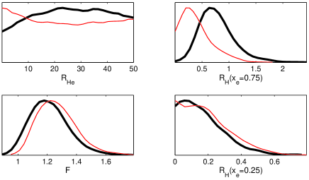
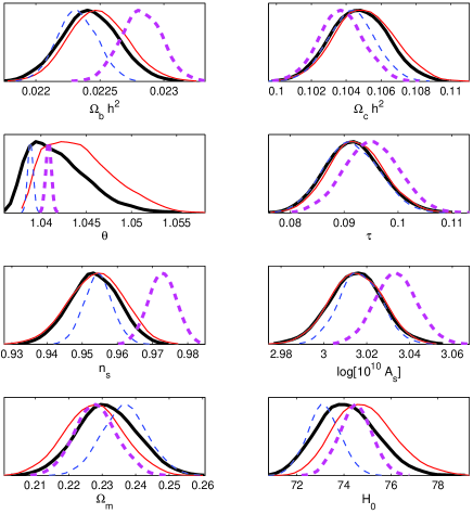
Figure 2: Forecast Planck constraints on recombination and cosmological parameters. There are two fiducial models, one using recfast (thin lines) and one using recfast with extra transitions following Dubrovich & Grachev (2005) (thick lines). Each simulated data set is analysed in two ways: dashed curves show the constraints using recfast and no additional recombination parameters; solid lines show the constraints allowing for four extra effective recombination parameters, as described in the text. The dotted lines show that using a fixed wrong recombination model can give biased parameter constraints; allowing for extra parameters (solid lines) broadens the errors bars but gives consistent results for both fiducial models.

Helium recombination is more complicated than hydrogen, but also less important: the significant difference between the HeI recombination histories only has a percent-level effect on the observed CMB spectrum on small scales due to the slightly modified diffusion damping length.

The dashed curves in Fig. 2 show the bias on parameter constraints from Planck if an incorrect recombination history is used that differs by as much as the Dubrovich & Grachev (2005) corrections to recfast. It should therefore be a matter of some priority to continue the work of  Seager et al. (2000) and Dubrovich & Grachev (2005); Chluba & Sunyaev (2006); Rubino-Martin et al. (2006) to include all transitions that might be important, and to quantify the importance of poorly known transition rates on the predictions.

In this paper we investigate the use of a crude ad hoc parameterization that can be used to obtain correct cosmological parameter constraints given the current level of uncertainties. We regard this as a proof of principle rather than a recommendation for practice. It may be a useful guide to where most effort needs to be concentrated to obtain more accurate results in future.

We base our calculations on the recfast code. We evolve these same equations, with modifications incorporating additional parameters. In recfast the effect of out of equilibrium distributions lead to a faster rate of hydrogen recombination than in a simple analysis. This is accounted for by multiplying the recombination coefficient by a ‘fudge factor’ F, fixed to 1.14 in recfast to match their full multi-level atom results. Other authors get slightly different values (Rubino-Martin et al., 2006). We take F to be a free parameter that effectively governs the speed of the end of recombination.

At earlier times recombination is dominated by the two-photon transitions, accounted for in recfast only from the lowest excited state. The calculation of Dubrovich & Grachev (2005) includes additional transitions from higher states, and there are also corrections from induced decay (Chluba & Sunyaev, 2006). We parameterize the uncertainties governing the two-photon transitions by using an effective two-photon rate $\Lambda_{\rm H}$ parameterized by

$$\Lambda_{\rm H}=\Lambda_{\rm H}^{(2)}\left[1+R_{H}(x_{e}=0.75)\left(\frac{R_{H}(x_{e}=0.25)}{R_{H}(x_{e}=0.75)}\right)^{2(0.75-x_{e})}\right].$$ (9)

Here $\Lambda_{\rm H}^{(2)}$ is the (fixed) empty-space 2s-1s two-photon rate, and the two parameters $R_{H}(x_{e}=0.75)$ and $R_{H}(x_{e}=0.25)$ measure an additional early and late contribution to the two-photon rate from extra transitions and induced decay. This model is not well motivated physically, but has the benefit of being fairly well constrained from the data. The exponential form allows it to capture exponential behaviour from Boltzmann-factors governing populations of excited states. Since the CMB is only weakly sensitive to the Helium recombination, we use the single parameter $R_{\text{He}}$ so that the effective two-photon Helium transition rate is given by $\Lambda_{\text{He}}=\Lambda_{\text{He}}^{(2)}R_{\text{He}}$. We do not change anything else. Although rather ad hoc, we expect that these parameters should be able to describe most changes to the recombination rate, and have a physical interpretation as measuring an effective rate at four different levels of ionization. Alternative parameterizations are discussed by Hannestad & Scherrer (2001).

Fig. 2 shows the parameter constraints from our Planck mean log likelihood forecasting function, using two different fiducial models of recombination. Including marginalization over the four additional recombination parameters allows the cosmological parameters to be extracted correctly in both cases, though with increased error bars. The posterior of the recombination parameters clearly shows that $R_{H}(x_{e}=0.75)$ and $F$ can be constrained away from zero, though the other two parameters are poorly constrained. With good polarization data the parameter $F$ is in fact very benign: varying only $F$ recovers cosmological parameters with essentially the same error bars as fixing it to 1.14 (the recfast value). However varying the rate of the two-photon hydrogen transitions shifts the redshift of maximum visibility, hence the large increase in the posterior range of $\theta$ that governs the positions of the acoustic peaks. Since our parameterization only allows for speeding up of transitions relative to recfast, the posterior distributions are non-Gaussian with a tail to larger $\theta$ corresponding to faster recombination, and a one-sided increase to the matter density posterior.

We have only considered basic 6-parameter cosmological models here, and more general models may be more degenerate with the recombination parameters, though a running spectral index can be constrained well even with the extra parameters.

Since details of recombination only significantly affect the small scale power spectrum, the impact of standard recombination uncertainties is rather mild when considering only the current WMAP three-year data: parameter constraints are affected only by a fraction of the error bar, comparable to the effects of different priors, likelihood modelling approximations, and secondary signals. For this reason we have not presented constraints on the recombination parameter space for WMAP; recfast is sufficiently accurate to obtain reliable parameters at the moment.

3.2 Non-standard models

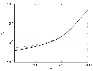
Figure 3: Ionization history for standard recfast (fudge parameter $F=1.14$, solid), recfast with $F=1$ (dash-dotted), and recfast with $F=1.14$ and an input of $3\times 10^{-24}\rm{eV}s^{-1}$ per proton today from homogeneous dark matter annihilation (dashed; see Padmanabhan & Finkbeiner (2005), equivalent to $F_{26}=0.06$ of Zhang et al. (2006)).

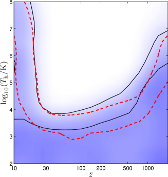
Figure 4: WMAP (solid line) and simulated PLANCK (dashed line) constraints on the parameter $T_{\rm h}$ as a function of redshift $\bar{z}$. Shading corresponds to the marginalized probability for the WMAP constraint and contours are at $68\%$ and $95\%$.

Our ad hoc parameterization may also pick up (and partly correct for) many non-standard processes, for example annihilating dark matter could inject energy during and after recombination. Low values for the free fudge parameter $F$ would be likely to fit these models better, corresponding to the increased ionization fraction at the end of recombination in these scenarios (Chen & Kamionkowski, 2004; Padmanabhan & Finkbeiner, 2005; Zhang et al., 2006). Figure 3 shows an ionization history with dark matter annihilation from Zhang et al. (2006), compared to a recfast history with lower value of the fudge parameter $F$. The shape at the tail end of recombination is somewhat similar, even though the (very small) ionization fraction at late times is significantly different. The resulting $C_{l}$ agree to below a percent except for few-percent change to the large-scale polarization signal. As we have seen $F$ can be constrained well, largely as a result of Planck’s good polarization sensitivity, so models with significant annihilation should also be clearly distinguishable. If we treat the annihilation rate as a free parameter, but fix recombination otherwise to recfast, our forecast for Planck suggests homogeneous rates today of $\gtrsim 3\times 10^{-24}\rm{eV}s^{-1}$ per proton will be detectable at $95\%$-confidence, consistent with the forecast of Padmanabhan & Finkbeiner (2005). This is also consistent with the constraint on the fudge parameter $F$ shown in Figure 2 when comparing the annihilation history with the similar $F=1$ model shown in Figure 3.

If the annihilation rate is much higher than that shown in Fig. 3 the fudge parameter $F$ will no longer be able to mimic the decay well. This is because higher annihilation rates give a significant contribution to the optical depth from the lower redshift ionization fraction, and also change the $l\lesssim 100$ polarization signal more radically. Such large annihilation rates should however be clearly distinguishable using an appropriate model.

Physically motivated dark matter candidates are generally expected have a small effect on the CMB power spectra due to decay or annihilation (Mapelli et al., 2006). Constraints on dark matter annihilation from recent data via the effect on the ionization history are given in Zhang et al. (2006); Mapelli et al. (2006), so we do not consider non-standard models any further here.

Ad hoc models for the injection of Lyman-$\alpha$ photons during recombination could also delay the time of maximum visibility (Peebles et al., 2001; Doroshkevich et al., 2003; Bean et al., 2003), so more general parameterizations allowing for slower recombination would be needed to pick up and account for more general models. Models which increase the ionization fraction significantly at quite low redshift can give rise to significant optical depth (Peebles et al., 2001; Doroshkevich et al., 2003; Bean et al., 2003). These models are likely to be ultimately quite well constrained by the large scale polarization signal as part of the recombination component.

An alternative way of modifying the precise details of recombination is to increase the temperature of the matter (baryons), $T_{\rm M}$, by the injection of energy, assuming the production of Lyman-$\alpha$ photons to be inefficient. Such a possibility has been considered previously in Weller et al. (1999) and achieves modifications to the ionization history by shifting the balance between recombination and cooling. A simple phenomenological model would be to consider the input of energy with a Gaussian profile centred around $\bar{z}$ with width $\rho$. This can be achieved by inclusion of an extra term in recfast (Eq. (7))

$${dT_{\rm M}\over dz}\bigg{|}_{\rm h}={T_{\rm h}\over\rho}\sqrt{2\over\pi}\exp\bigg{[}-{2(z-\bar{z})^{2}\over\rho^{2}}\bigg{]}\,,$$ (10)

which, in the absence of any cooling processes and assuming that ${\bar{z}}>>\rho$, would lead to an increase in the matter temperature $\Delta T_{\rm M}=T_{\rm h}$. This would require the input of a total energy of $8.6{\rm eV}(T_{\rm h}/10^{5}{\rm K})$ per baryon over the period of heating. In any given scenario cooling processes will suppress the effect substantially, but it is still possible to increase the temperature of the IGM enough for it to have an observable effect on the CMB anisotropies.

We have investigated the constraint imposed by the current WMAP data on $T_{\rm h}$ as a function of ${\bar{z}}$, marginalizing over $0.05<\rho/{\bar{z}}<0.3$ and the results are presented in Fig. 4. We see that for late (${\bar{z}}<30$) and early times (${\bar{z}}>1100$) large amounts of energy ($T_{\rm h}>10^{7}{\rm K}$) can be input without changing the CMB anisotropies; at low redshift heating effects are swamped by reionization. Large heat inputs may be constrained in other ways, for example, by spectral distortions in the CMB, however any reasonable heat input is not constrained by observational limits on spectral distortions (Weller et al., 1999). There are tight constraints of $T_{\rm h}<10^{4}{\rm K}$ for $30<\bar{z}<100$, $T_{\rm h}<10^{5}{\rm K}$ for $100<{\bar{z}}<500$ and $T_{\rm h}<10^{6}{\rm K}$ for $z\sim 1000$ (all limits are $2\sigma$).

By considering a fiducial model with $T_{\rm h}=0$, we have also used simulated Planck likelihood functions to show that more stringent constraints will be possible in the near future in the range $200<{\bar{z}}<1500$, as show by the dashed lines in Fig. 4.

4 Reionization

4.1 Binning the ionization fraction

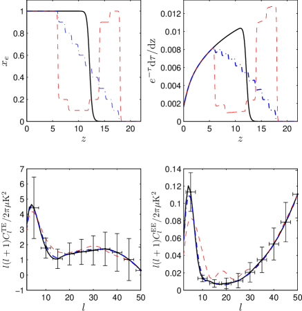
Figure 5: CMB anisotropies and ionization histories for the fiducial models used in this analysis: sharp (solid), dashed (double reionization) and dragged (dash-dotted). The total optical depth for all three models is $\tau=0.1$. The top left panel is the ionization fraction $x_{e}$, top right is the visibility (with respect to $z$). Bottom left are the temperature-polarization cross-correlation power spectra, bottom right the $E$-polarization power spectra. Error bars on the bottom plots show the noise plus cosmic variance from our simple model of Planck in the sharp reionization model.

In order to constrain the reionization history of the Universe we bin the ionization fraction in redshift bins with

$$x_{e}(z)=x_{i}\;,\qquad z_{i}-\frac{\Delta z}{2}<z<z_{i}+\frac{\Delta z}{2}\;.$$ (11)

We further introduce a maximum redshift $z_{\rm max}$ above we follow the standard recombination history without reionization and a minimum redshift $z_{\rm min}$ below which we assume complete reionization. In practice we require the ionization history to be smooth, so we join the bins using a $\tanh$-function. We neglect Helium reionization at $z\sim 3$ as this only has a very small effect on the CMB. Note that since a constant $x_{e}$ electron density falls off as $n_{e}\propto(1+z)^{3}$ in matter domination, the visibility per redshift interval scales like $(1+z)^{1/2}$, and hence $x_{e}$ bins of fixed redshift width contribute somewhat more to the optical depth at higher redshift. The choice of best bin widths and offset is not obvious without any clear theoretical priors on the expected reionization history. These could be taken as additional parameters, but for simplicity we fix them here; we choose the first bin to start at $z\sim 6$ where we think the ionization fraction first was last significantly less than unity. If the binning is in phase with any features in the ionization history the reconstruction will be much cleaner. It may therefore be a good idea to use two separate reconstructions offset by half a bin for comparison.

We consider three fiducial reionization histories that all have an optical depth $\tau\approx 0.1$. The first is a “standard” reionization history with sharp complete reionization at a redshift $z\sim 12$. The second scenario is a dragged out reionization and the third a double reionization scenario (for possible physical models and discussion see Cen (2003); Furlanetto & Loeb (2005)). The latter two are modelled using a series of narrow bins in redshift adjusted to give the same total optical depth. Other cosmological parameters are set to the values for the best fit six parameter WMAP three-year concordance model (Spergel et al., 2006).

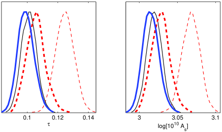
Figure 6: Planck optical depth and amplitude constraints from the sharp model analysed using the sharp model (thin solid), the incorrect result from analysing a double reionization model using a sharp model (thin dashed), and the consistent result from the double reionization (thick dashed) and sharp (thick solid) models using a binned reconstruction.

Figure (5) shows the reionization histories and polarization power spectra for the three fiducial models. The temperature power spectra are virtually identical, so polarization information is essential. The accuracy with which the spectra can be measured is limited by cosmic variance on these large scales even if noise and foreground uncertainties were negligible. This limits the amount of information that can be extracted from the CMB even with perfect data. The fast and dragged reionization histories give rather similar power spectra, however the double reionization history, which has two distinct peaks in the visibility function, gives a clearly different prediction (for further discussion see Hu & Holder (2003)). If fast reionization is assumed, the inferred optical depth would be incorrect if in reality there is double reionization (Holder et al., 2003), as shown in Figure 6. Since the small scale $C_{l}$ scales with the amplitude as $A_{s}e^{-2\tau}$, an incorrect optical depth also means that the CMB constraint on the amplitude (and hence e.g. $\sigma_{8}$) would also be incorrect. Modelling the reionization history therefore has the joint aims of learning as much as we can about how the universe reionized, at the same time as allowing other cosmological parameters to be constrained reliably.

4.2 Binning priors

It is important to be aware of ones priors when using different parameterizations. In particular, when binning some function, introducing many new parameters with flat amplitude priors can correspond to unintended priors on other parameters. For example, consider the case when we somehow measure only the total optical depth $\tau$. When $\tau$ is the only parameter we might get $\tau=\tau_{0}\pm\sigma$, and for simplicity suppose the posterior is Gaussian. Now say we bin the reionization history in $N$ bins that contribute equally to the optical depth so that $\tau=\sum_{n}\tau_{n}$. Then if each bin posterior is uncorrelated and Gaussian we have $\tau_{n}=\tau_{0}/N\pm\sigma/\sqrt{N}$: we have measured each bin to have about the same small contribution to the optical depth without having any relevant data! This reflects the much larger parameter space volume where all the bins have approximately the same contribution than when most of the contribution is coming from just a few bins.

Looking at it the other way, consider $N$ bins with total optical depth $\tau=\sum_{n}\tau_{n}$ where $0<\tau_{n}<\tau_{n}^{(1)}\equiv\tau_{n}(x_{e}=1)$, so we treat the contributions to $\tau$ as though independent. If we have a flat prior on $x_{e}$ in each bin with $0\leq x_{e}\leq 1$, we have a flat prior on the optical depth from each bin of $P(\tau_{n})=1/\tau_{n}^{(1)}$ for $0\leq\tau_{n}\leq\tau_{n}^{(1)}$ (and zero otherwise). The prior on the total $\tau$ is then

$$P(\tau) = \int\rm{d}\tau_{0}\dots\int\rm{d}\tau_{N}\,\delta\left(\tau-\sum_{n}\tau_{n}\right)\prod_{n=1}^{N}P(\tau_{n})$$ (12)

$$= \int_{-\infty}^{\infty}\frac{\rm{d}k}{2\pi}e^{ik\tau}\prod_{n=1}^{N}\left[\int\rm{d}\tau_{n}P(\tau_{n})e^{-ik\tau_{n}}\right]$$

$$= \int_{-\infty}^{\infty}\frac{\rm{d}k}{2\pi}e^{ik\tau}\prod_{n=1}^{N}\left[\frac{e^{-ik\tau_{n}^{(1)}}-1}{-ik\tau_{n}^{(1)}}\right]$$

$$\sim \frac{1}{\sqrt{2\pi\sigma^{2}}}e^{-(\tau-\bar{\tau})^{2}/2\sigma^{2}}.$$

The exact integral gives a prior for $\tau$ that is piecewise polynomial, peaking at $\bar{\tau}\equiv\sum_{n}\tau_{n}^{(1)}/2$ and with variance $\sigma^{2}\equiv\sum_{n}\tau_{n}^{(1)}{}^{2}/12$. This approximates a Gaussian for large $N$. For bins with equal $\tau^{(1)}$ the exact result is

$$P(\tau)=\sum_{n=0}^{N}\frac{(\tau/\tau^{(1)}-n)^{N}}{|\tau-n\tau^{(1)}|}\frac{(-1)^{n}N}{2(N-n)!n!}.$$ (13)

Assuming we are in the region where the posterior favours $\tau<\bar{\tau}$, the binning prior will therefore favour higher values of $\tau$ than using a flat prior on $\tau$. For $\tau$ close to zero the prior goes like $\tau^{N-1}$: you are very unlikely to get all the bins very close to zero. A good data constraint generally has an exponential likelihood function, so the prior is only logarithmically important compared to the log likelihood, however for large numbers of bins the prior can have a significant effect. In the absence of a strong constraint from the data, assuming a flat prior on a large set of reionization bins will therefore favour posterior constraints where each bin has a small contribution to the optical depth and the total $\tau$ is higher than you would get from no binning. It is important to use as much prior information as possible to get relevant results: If you use a prior you don’t believe, you shouldn’t in general believe the posterior either.

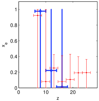
Figure 7: Reionization fraction from WMAP 3-year data using seven bins with $\Delta z=3$ (thin lines) and three bins with $\Delta z=4$ (thick lines, $x_{e}$ assumed zero at $z>18$). Vertical error bars show $68\%$ confidence regions. The results are largely prior driven, but bin correlations are $\lesssim 0.2$.

4.3 Results

Figure 7 shows the constraint from current WMAP data (Hinshaw et al., 2006; Page et al., 2006) when three and seven reionization bins are used. The WMAP polarization results are noise dominated, so the constraint is very weak. As shown in the figure, the conclusions one might come to depend on the prior: using more bins indicates that the ionization fraction is constrained to be lower at intermediate redshift than when using only three, if one considers the allowed $1-\sigma$ regions. With only WMAP data the result is largely prior driven. Since most people’s prior does not correspond to a random set of amplitudes in seven bins (e.g. most people probably expect at most one local maximum), most people should not believe the result. When better data is used the effect of an unbelievable prior is much less important, but can still pull results in a direction you don’t really believe. An alternative parameterization using a bin with a free $z_{\text{max}}$ is described in Spergel et al. (2006), though this is not significantly constrained by the data either (as expected  (Kaplinghat et al., 2003)).

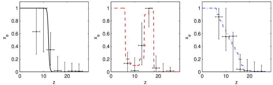
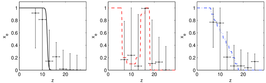
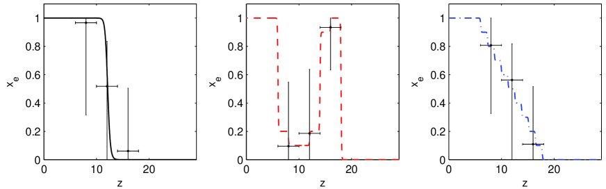
Figure 8: Reconstructed reionization bins from perfect data (top) and Planck (middle and bottom) for the three fiducial models. Points show maximum sample likelihood positions, vertical error bars are the marginalized $95\%$ confidence intervals, and the horizontal bars show the width of the redshift bins ($\Delta z=3$ top two plots, $\Delta z=4$ for bottom plot). The lines show the fiducial input model ionization history in each case. The bottom panel shows a Planck reconstruction for three bins with a prior that $x_{e}=0$ at $z>18$. Adjacent bins away from zero are correlated at the $0.3$–$0.7$ level.

In order to test how well CMB observations can constrain reionization in principle we assume that all cosmological parameters, apart from the bins in the ionization fraction, are fixed. We then use the mean log likelihood from noise-free full-sky data to forecast the reconstruction constraints, using data from $l\leq 100$ where the reionization signal is important. We use $z_{\rm min}=7$, $z_{\rm max}=25$ and $\Delta z=3$. In the top panel of Figure 8 we show the reconstructed ionization histories for the three fiducial models. From these plots we see that for perfect data we can distinguish the double reionization scenario from the other two fiducial models at many sigma. Note however that the error bars are correlated, and any detailed hypothesis test should take this into account or work directly from the chains. Models can be distinguished even if they appear consistent in a marginalized error-bar plot: the regions in the full $n$-dimensional parameter space may be different even if the projections are the same. A reionization binning is a nice way to see what sharp redshift information is available, but models that differ by broader features (for example the sharp and dragged models) may be better modelled using a more targeted parameterization — for example a couple of parameters governing the slope of $x_{e}$ as it goes from $x_{e}=1$ at $z\sim 6$ to zero at higher redshift.

We next include noise expected from the Planck satellite and allow the other cosmological parameters to vary. The result is shown in the middle panel of Figure 8. It is hard to distinguish the three fiducial models at the 2-$\sigma$ level by comparing a number of marginalized reionization redshift bin constraints. This is largely because there is a degeneracy between the bins over the reionization peak: Planck cannot resolve the redshift of the start of reionization accurately enough to distinguish high $x_{e}$ followed by low $x_{e}$ from the case where two bins contribute more equally. This is apparent in the (anti-)correlation of the error bars: when $x_{e}$ is significant there is a $\sim 0.3$ anti-correlation between adjacent points. If we include a prior that $x_{e}=0$ at $z>18$, the constraint using $\Delta z=4$ bins looks much better (bottom panel of Figure 8), though the bins are now fine-tuned to a priori knowledge about the expected form of the history. Bin anti-correlations are still large at $\sim 0.5$–$0.7$. Our conclusions are not changed significantly if we instead fix the cosmological parameters: Planck constrain the other parameters well, and on large scales the reconstruction is noise and cosmic variance limited.

The constraint on $\tau$ when seven bins are used is consistent with the fiducial value, whichever ionization history is used: see Figure 6. Note that our analysis is assuming statistical isotropy; if the large scale CMB is not isotropic as suggested by numerous analyses of the WMAP data, it may be much harder to model or learn anything about the late time ionization history. Alternatively it is possible that the signal from a well understood ionization history could be used to learn more about the structure of the large scale universe.

An alternative to our binned parameterization would be to use a reduced set of well constrained Fisher PCA components identified by Hu & Holder (2003). However these have unphysical negative ionization fractions, and the physical interpretation is clearer in easily distinguishable models using our direct redshift binning. Also the PCA components depend on the fiducial model (or an iterative scheme), so a one-off binned parameter run is simpler to use in practice. We have investigated the extraction of PCA components from our posterior bin parameter chains, however the results we obtained appear not to be very useful and rather different from the Fisher components of Hu & Holder (2003). This can be partly explained because infinitesimal derivatives about a fiducial model generally give different covariance estimates than samples from posteriors generated using physical priors (e.g. that $0\leq x_{e}\leq 1$) accounting for the full non-Gaussian posterior shape.

5 Conclusions

Modelling the ionization history is crucial to interpret high precision observations of the CMB correctly. Uncertainties in the details of recombination affect the small scale anisotropies, and an incorrect model can lead to strongly biased parameter constraints. We have made a first step towards modelling recombination uncertainties using an ad hoc parameterization governing the recombination rate at four different ionization fractions. This was good enough to recover parameter estimates that are consistent, but at the cost of larger error bars. There is clear motivation for future work to pin down the recombination history in more detail theoretically, with quantification of errors on any poorly measured important parameters. In principle future work could do a full multi-atom calculation for each cosmological model, including free parameters with error bars for all rates that are not known very accurately. In practice it is likely to be possible to devise an accurate small set of effective equations that can be evolved quickly, along the lines of the current recfast code. Using a free parameterization has the advantage of being able to look for any surprises, for example energy injection from annihilating particles, however if the standard model predictions are not well nailed down it may be hard to distinguish subtle unexpected effects from uncertainties in the expected model.

The reionization impacts the large scale CMB polarization anisotropies. Our conclusions effectively agree with previous work, though our direct binning approach is somewhat different. Ideal data can do quite well at distinguishing distinct models, and even Planck may be able to separate the most clear-cut cases. We concentrate on Planck, also there are ground based probes which could provide useful information about reionization. In particular the Background Imaging of Cosmic Extragalactic Polarization (BICEP) has in principle the ability to measure features in the first trough in the E-mode anisotropies, which at least to some degree could constrain the details of the reionization history (Keating et al., 2003). However the error bars remain quite large even with ideal data, and the CMB is ultimately not going to be the best way to learn about the reionization history observationally: 21cm emission is likely to be a much better tracer. Allowing for different models in a CMB analysis is however crucial to obtain unbiased constraints on the optical depth (and hence the underlying perturbation variance) if the optical depth is quite large. Of course if the optical depth is observed to be low, so we know reionization must all have happened around $z\sim 6$, the modelling for the history becomes less important as there is then little room more complicated reionization scenarios. Alternatively a consensus may arise that the reionization history is expected to be monotonic (e.g. see Furlanetto & Loeb (2005)), in which case modelling is less important and significantly simpler.

6 Acknowledgements

We thank Douglas Scott, Wan Yan Wong, Steven Gratton, George Efstathiou and Anthony Challinor for discussion and Xuelei Chen for his modified version of camb. Most computations were performed on CITA’s Mckenzie cluster (Dubinski et al., 2003) which was funded by the Canada Foundation for Innovation and the Ontario Innovation Trust. We acknowledge the use of the Legacy Archive for Microwave Background Data Analysis (LAMBDA). Support for LAMBDA is provided by the NASA Office of Space Science. AL is supported by a PPARC Advanced Fellowship.

References

- Alvarez et al. (2006) Alvarez M. A., Shapiro P. R., Ahn K., Iliev I. T., 2006, ApJ, 644, L101, astro-ph/0604447
- Bean et al. (2003) Bean R., Melchiorri A., Silk J., 2003, Phys. Rev., D68, 083501, astro-ph/0306357
- Becker et al. (2001) Becker R. H., et al., 2001, AJ, 122, 2850, astro-ph/0108097
- Cen (2003) Cen R., 2003, ApJ, 591, 12, astro-ph/0210473
- Chen & Kamionkowski (2004) Chen X.-L., Kamionkowski M., 2004, Phys. Rev., D70, 043502, astro-ph/0310473
- Chluba & Sunyaev (2006) Chluba J., Sunyaev R. A., 2006, A&A, 446, 39, astro-ph/0508144
- Doroshkevich et al. (2003) Doroshkevich A. G., Naselsky I. P., Naselsky P. D., Novikov I. D., 2003, ApJ, 586, 709, astro-ph/0208114
- Dubinski et al. (2003) Dubinski J., Humble R., Pen U.-L., Loken C., Martin P., 2003, astro-ph/0305109
- Dubrovich & Grachev (2005) Dubrovich V. K., Grachev S. I., 2005, Astronomy Letters, 31, 359, astro-ph/0501672
- Fan et al. (2006) Fan X.-H., Carilli C. L., Keating B., 2006, astro-ph/0602375
- Furlanetto & Loeb (2005) Furlanetto S., Loeb A., 2005, ApJ, 634, 1, astro-ph/0409656
- Gnedin & Fan (2006) Gnedin N. Y., Fan X.-H., 2006, astro-ph/0603794
- Hannestad & Scherrer (2001) Hannestad S., Scherrer R. J., 2001, Phys. Rev., D63, 083001, astro-ph/0011188
- Hinshaw et al. (2006) Hinshaw G., et al., 2006, astro-ph/0603451
- Holder et al. (2003) Holder G., Haiman Z., Kaplinghat M., Knox L., 2003, ApJ, 595, 13, astro-ph/0302404
- Hu (2000) Hu W., 2000, ApJ, 529, 12, astro-ph/9907103
- Hu & Dodelson (2002) Hu W., Dodelson S., 2002, Ann. Rev. Astron. Astrophys., 40, 171, astro-ph/0110414
- Hu & Holder (2003) Hu W., Holder G. P., 2003, Phys. Rev., D68, 023001, astro-ph/0303400
- Hu et al. (1995) Hu W., Scott D., Sugiyama N., White M. J., 1995, Phys. Rev., D52, 5498, astro-ph/9505043
- Kaplinghat et al. (2003) Kaplinghat M., et al., 2003, ApJ, 583, 24, astro-ph/0207591
- Keating et al. (2003) Keating B. G., Ade P. A. R., Bock J. J., Hivon E., Holzapfel W. L., Lange A. E., Nguyen H., Yoon K. W., 2003, in Fineschi S., ed., Polarimetry in Astronomy. Proceedings of the SPIE, Volume 4843. BICEP: a large angular scale CMB polarimeter. pp 284–295
- Leung et al. (2004) Leung P. K., Chan C.-W., Chu M.-C., 2004, MNRAS, 349, 632, astro-ph/0309374
- Lewis (2005) Lewis A., 2005, Phys. Rev., D71, 083008, astro-ph/0502469
- Lewis & Bridle (2002) Lewis A., Bridle S., 2002, Phys. Rev., D66, 103511, astro-ph/0205436
- Lewis & Challinor (2006) Lewis A., Challinor A., 2006, Phys. Rept., 429, 1, astro-ph/0601594
- Lewis et al. (2000) Lewis A., Challinor A., Lasenby A., 2000, ApJ, 538, 473, astro-ph/9911177
- Loeb & Barkana (2001) Loeb A., Barkana R., 2001, Ann. Rev. Astron. Astrophys., 39, 19, astro-ph/0010467
- Mapelli et al. (2006) Mapelli M., Ferrara A., Pierpaoli E., 2006, MNRAS, 369, 1719, astro-ph/0603237
- Padmanabhan & Finkbeiner (2005) Padmanabhan N., Finkbeiner D. P., 2005, Phys. Rev., D72, 023508, astro-ph/0503486
- Page et al. (2006) Page L., et al., 2006, astro-ph/0603450
- Peebles (1968) Peebles P. J. E., 1968, ApJ, 153, 1, ADS
- Peebles (1993) Peebles P. J. E., 1993, Principles of physical cosmology. Princeton University Press, ISBN: 0691019339, ADS
- Peebles et al. (2001) Peebles P. J. E., Seager S., Hu W., 2001, ApJ, 539, L1, astro-ph/0004389
- Planck (2006) Planck 2006, astro-ph/0604069
- Popa (2006) Popa L. A., 2006, astro-ph/0605358
- Rubino-Martin et al. (2006) Rubino-Martin J. A., Chluba J., Sunyaev R. A., 2006, astro-ph/0607373
- Seager et al. (1999) Seager S., Sasselov D. D., Scott D., 1999, ApJ, 523, L1, astro-ph/9909275
- Seager et al. (2000) Seager S., Sasselov D. D., Scott D., 2000, ApJS, 128, 407, astro-ph/9912182
- Seljak & Zaldarriaga (1996) Seljak U., Zaldarriaga M., 1996, ApJ, 469, 437, astro-ph/9603033
- Spergel et al. (2006) Spergel D. N., et al., 2006, astro-ph/0603449
- Weller (1999) Weller J., 1999, ApJ, 527, L1, astro-ph/9908033
- Weller et al. (1999) Weller J., Battye R. A., Albrecht A., 1999, Phys. Rev., D60, 103520, astro-ph/9808269
- Zahn et al. (2005) Zahn O., Zaldarriaga M., Hernquist L., McQuinn M., 2005, ApJ, 630, 657, astro-ph/0503166
- Zhang et al. (2006) Zhang L., Chen X.-L., Lei Y.-A., Si Z.-G., 2006, astro-ph/0603425