Magnetohydronamic Evolution of HII Regions in Molecular Clouds: Simulation Methodology, Tests, and Uniform Media

Abstract

We present a method for simulating the evolution of HII regions driven by point sources of ionizing radiation in magnetohydrodynamic media, implemented in the three-dimensional Athena MHD code. We compare simulations using our algorithm to analytic solutions and show that the method passes rigorous tests of accuracy and convergence. The tests reveal several conditions that an ionizing radiation-hydrodynamic code must satisfy to reproduce analytic solutions. As a demonstration of our new method, we present the first three-dimensional, global simulation of an HII region expanding into a magnetized gas. The simulation shows that magnetic fields suppress sweeping up of gas perpendicular to magnetic field lines, leading to small density contrasts and extremely weak shocks at the leading edge of the HII region’s expanding shell.

1. Introduction

Observations show that giant molecular clouds (GMCs) in local group galaxies convert at most a few percent of their mass into stars per cloud crossing time (Zuckerman & Evans, 1974), and that clouds are typically destroyed in a few crossing times (Blitz et al., 2005), well before they have converted a significant fraction of their mass into stars. Observations also strongly support the idea that GMCs are gravitationally bound (Krumholz & McKee, 2005; Blitz et al., 2005; Krumholz et al., 2006), so the fact that they survive for more than a crossing time yet do not collapse entirely into stars strongly suggests that internal feedback plays a dominant role in GMC evolution. HII regions driven by newly-formed massive stars are likely to be the dominant sources of energy injection and mass loss in clouds, and are therefore critical to GMC evolution (McKee & Williams, 1997; Williams & McKee, 1997; Matzner, 2002). Krumholz et al. (2006) show using semi-analytic models that feedback from HII regions can quantiatively reproduce the observed lifetime, star formation rate, and star formation efficiency of GMCs. However, these calculations rely on simple analytic solutions for the evolution of spherically-symmetric HII regions in non-magnetic gas. Understanding the detailed evolution of GMCs will require a considerably more sophisticated numerical approach, and for this reason three-dimensional simulation of the evolution of molecular clouds under the influence of internal sources of ionizing radiation is a critical problem in numerical astrophysics.

In this paper we have the dual purpose of presenting a new algorithm for simulation of HII regions in molecular clouds, and using this algorithm to explore potential computational problems that arise in general for simulations of this type. We also demonstrate our new algorithm in a simple application, the expansion of an HII region into a uniform neutral gas in which the magnetic pressure greatly exceeds the thermal pressure, as it does in molecular clouds. In the past year several authors have considered the problem of simulating HII regions, and presented both algorithms (e.g. Arthur & Hoare, 2006; Mellema et al., 2006) and results on the evolution of HII regions in turbulent hydrodynamic media (Dale et al., 2005; Mellema et al., 2005; Mac Low et al., 2006). For a recent review see Henney (2006). Several authors have also presented methods for simulation of ionizing radiation-hydrodynamics (IRHD) in a cosmological context (e.g. Abel & Wandelt, 2002; Whalen & Norman, 2006), which differs from the problem in the context of present-day molecular clouds primarily in the amount of cooling to which the gas is subjected and the conditions of the gas before it is ionized. Finally, researchers studying the evolution of ultracompact HII regions planetary nebulae have presented algorithms and results for ionizing radiative transfer with hydrodynamics and magnetohydrodynamics in 2D and 3D under the simplifying assumption that the ionized gas has a perfectly sharp edge and is always in thermal and ionization equilibrium (e.g. Garcia-Segura & Franco, 1996; Garcia-Segura, 1997; García-Segura & López, 2000).

Our algorithm improves on previous work in that it is the first to couple ionizing radiative transfer to magnetohydrodynamics (IRMHD) without imposing an assumption of thermal or ionization equilibrium. The inclusion of magnetic fields is important because observations indicate that the magnetic energy in molecular clouds is comparable to the kinetic and gravitational potential energies (Crutcher, 1999, 2005; Heiles & Crutcher, 2005). Thus, dynamical expansion of ionized regions may be significantly altered by magnetic confinement, an effect we wish to explore. Indeed, we show that even in the simple case of expansion of an HII region into a uniform, magnetized medium, the magnetic field produces qualitatively new phenomena. The Alfven speeds of a few km s^-1 typically found in molecular clouds reduce the strength of shocks associated with expanding ionization fronts at early times, and at later times turn off the shocks entirely, greatly reducing the collection of gas and possibly thereby reducing the amount of triggered star formation. A non-equilibrium treatment of the ionization structure is important because we find that a non-equilibrium treatment of the thermal and ionization structure of the ionized gas leads to modest but significant effects on quantities such as the expansion rate of HII regions, effects that are lost in the assumption of perfect radiative equilibrium.

Before exploring these new phenomena, however, we point out that there has yet to be a detailed study of potential computational problems and constraints that arise in 3D simulations of IRHD and IRMHD with the strong cooling and large temperature contrasts that are expected for modern day (as opposed to primordial) interstellar chemistry. We have therefore performed a detailed comparison of simulations using our method to analytic solutions for computationally challenging problems, as a way of searching for potential difficulties that may arise in general IRHD methods. We discover several conditions that a simulation must satisfy to reproduce analytic results correctly. One must limit the amount by which the gas pressure is allowed to change between hydrodynamic updates, for a ray-tracing method one must periodically rotate the orientation of the rays, and one must either resolve the ionization front or restrict the rate of cooling at the front to suppress excess cooling due to numerical mixing. We show that failure to meet these conditions produces quantitatively incorrect results.

The remainder of this paper proceeds as follows. In § 2 we describe the physical formulation of the problem that we adopt, including our approximations and assumptions. In § 3 we present our simulation algorithm. In § 4 we compare our code to analytic solutions, and thereby demonstrate the existence of conditions that numerical methods must satisfy in order to reproduce analytic solutions correctly. We use our method to simulate the evolution of HII regions in magnetized media in § 5, and finally we summarize and present conclusions in § 6.

2. Physical Formulation

We wish to simulate the evolution of a magnetized molecular gas subjected to an ionizing radiation field due to point sources within it. The $n$ sources of ionization are located at positions $\mathbf{x}_{n}$, and each has an ionizing luminosity of $s_{n}$, in units of photons per unit time above the Lyman limit. We treat the ionizing sources as monochromatic, and assume that they emit all their ionizing photons at frequencies near the ionization threshhold of hydrogen. Since our focus is on the dynamics of the cloud rather than the detailed chemistry of the ionized gas, this approximation is quite reasonable.

We describe the gas by a total mass density $\rho$, density of neutral species $\rho_{n}$, velocity $\mathbf{v}$, and total energy density $E$. The gas is threaded by a magnetic field $\mathbf{B}$. The interface between an HII region and a molecular cloud is a photodissociation region (PDR), within which there is a significant amount of atomic gas. In principle we should therefore separately track ionized, atomic, and molecular hydrogen, and possibly other species as well. However, PDRs do not have a signicant effect on the large-scale dynamics of the ionized gas unless the ionizing source is very weak or the neutral gas is much less dense than as typical for molecular clouds, as we show in § 2.4. For this reason, we neglect atomic gas, and assume that the density of molecular gas is $\rho_{n}$ and the density of ionized gas is $\rho-\rho_{n}$.

2.1. Magnetohydrodynamics

We compute the evolution of our gas using the equations of multi-species ideal MHD including radiative heating and cooling and chemical evolution terms. In conservative form, these are

$$\frac{\partial\rho}{\partial t}+\nabla\cdot(\rho\mathbf{v}) = 0$$ (1)

$$\frac{\partial}{\partial t}(\rho\mathbf{v})+\nabla\cdot(\rho\mathbf{v}\mathbf{v}-\mathbf{B}\mathbf{B})+\nabla P^{*} = 0$$ (2)

$$\frac{\partial\mathbf{B}}{\partial t}+\nabla\cdot(\mathbf{v}\mathbf{B}-\mathbf{B}\mathbf{v}) = 0$$ (3)

$$\frac{\partial E}{\partial t}+\nabla\cdot\left[(E+P^{*})\mathbf{v}-\mathbf{B}(\mathbf{B}\cdot\mathbf{v})\right] = \mathcal{G}-\mathcal{L}$$ (4)

$$\frac{\partial\rho_{n}}{\partial t}+\nabla\cdot(\rho_{n}\mathbf{v}) = \mathcal{R}-\mathcal{I},$$ (5)

where $P^{*}\equiv P+(\mathbf{B}\cdot\mathbf{B})/2$ is the total pressure, $P$ is the gas thermal pressure, $\mathcal{R}$ and $\mathcal{I}$ are the rates of recombination and ionization, measured in mass per unit time per unit volume, and $\mathcal{G}$ and $\mathcal{L}$ are the rates of radiative heating and cooling, in energy per unit time per unit volume. The total energy density $E$ not including atomic or molecular binding energies is

$$E\equiv\epsilon+\rho\frac{\mathbf{v}\cdot\mathbf{v}}{2}+\frac{\mathbf{B}\cdot\mathbf{B}}{2},$$ (6)

where $\epsilon$ is the gas thermal energy density. We adopt an ideal gas equation of state, so the pressure is $P=(\gamma-1)\epsilon$ with $\gamma=5/3$, corresponding to a monatomic gas. This choice of $\gamma$ is appropriate because ionized gas is monatomic, and hydrogen in molecular clouds, while diatomic, is generally too cool to access its rotational or vibrational degrees of freedom. It therefore acts as if it were monatomic for the purpose of dynamics. In addition to the evolution equations, the magnetic field is subject to the divergence-free constraint

$$\nabla\cdot\mathbf{B}=0.$$ (7)

Physically, equations (1), (2), and (4) represent conservation of mass, momentum, and energy, equation (3) represents the approximation that the magnetic field is perfectly frozen in to the fluid, and equation (5) states that the mass of neutral gas is conserved by advection, and is altered only by ionizations and recombinations. Equation (7) expresses the non-existence of magnetic monopoles. Note that we have adopted a system of units in which the magnetic permeability $\mu=1$; to convert to cgs units, we multiply our magnetic field strengths by a factor of $\sqrt{4\pi}$.

2.2. Recombination and Ionization

To complete the evolution equations, we must specify the rates of the radiative processes: recombination, ionization, heating, and cooling. Recombination is the simplest of these. We adopt the on-the-spot approximation whereby any recombination to the ground state of hydrogen is assumed to yield an ionizing photon with a very short mean free path, which will in turn cause another ionization at essentially the same location as the recombination (Osterbrock, 1989). On the other hand, recombinations to excited states of hydrogen produce photons with long mean free paths, which are assumed to escape the HII region. Thus, the recombination rate is approximately

$$\mathcal{R}=\mu_{H}\alpha^{(B)}n_{e}n_{H^{+}},$$ (8)

where $\mu_{H}\approx 2.34\times 10^{-24}$ g is the mean gas mass per hydrogen atom (for a gas of hydrogen and helium in the standard cosmic abundance), $n_{e}$ and $n_{H^{+}}$ are the number densities of electrons and hydrogen nuclei, and $\alpha^{(B)}$ is the case B recombination coefficient, $\alpha^{(B)}\approx 2.59\times 10^{-13}(T/10^{4}\mbox{ K})^{-0.7}$ cm^-3 s^-1 (Osterbrock, 1989; Rijkhorst et al., 2005) at a gas temperature $T$. The H⁺ and e^- number densities are $n_{H^{+}}=(\rho-\rho_{n})/\mu_{H}$ and $n_{e}=n_{H^{+}}+\rho\alpha_{C}/(14\mu_{H})$, where $\alpha_{C}\approx 3\times 10^{-3}$ is the carbon abundance in the ISM (Sofia & Meyer, 2001). This assumes that all carbon is singly-ionized. Since the first ionization potential of carbon is smaller than that of hydrogen, this is likely to be the case in regions where there is any ionized hydrogen present, which are the only regions for which we care about the recombination rate.

In the on-the-spot approximation, the ionization rate is relatively easy to compute as well, since we need only solve the radiative transfer equation only along rays from ionizing sources. The ionizing flux at position $\mathbf{x}$ due to the $n$th ionizing source is

$$F_{n}=\frac{s_{n}}{4\pi\left|\mathbf{x}-\mathbf{x}_{n}\right|^{2}}e^{-\tau(\mathbf{x},\mathbf{x}_{n})},$$ (9)

where

$$\tau(\mathbf{x},\mathbf{x}_{n})\approx\int_{\mathbf{x}_{n}}^{\mathbf{x}}(\sigma n_{H}+\sigma_{d}n)\,d\ell$$ (10)

is the optical depth to ionizing photons along the path from $\mathbf{x}_{n}$ to $\mathbf{x}$, $n_{H}=\rho_{n}/\mu_{H}$ is the number density of neutral hydrogen atoms, $n=\rho/\mu_{H}$ is the number density of hydrogen nuclei, $\sigma=6.3\times 10^{-18}$ cm² is the cross section for absorption of a photon at the ionization threshhold by a neutral hydrogen atom, and $\sigma_{d}\approx 6.1\times 10^{-22}$ cm^-2 per H atom is the cross section for absorption of ionizing photons by dust grains (Bertoldi & Draine, 1996). For the purposes of the tests we report in this paper, for which we are comparing to analytic solutions derived for pure hydrogen, we set $\sigma_{d}=0$. The photoionization rate is just the rate at which these photons are absorbed, so the total photoionization rate due to all sources at position $x$ is

$$\mathcal{I}_{\rm ph}=\sigma\rho_{n}\sum_{n}\frac{s_{n}}{4\pi\left|\mathbf{x}-\mathbf{x}_{n}\right|^{2}}e^{-\tau(\mathbf{x},\mathbf{x}_{n})}.$$ (11)

We also compute the rate of ionizations due to collisions between neutral hydrogen atoms and electrons,

$$\mathcal{I}_{\rm coll}\approx k_{\rm coll}n_{e}\rho_{n},$$ (12)

where the collisional ionization rate coefficient is (Tenorio-Tagle et al., 1986)

$$k_{\rm coll}\approx 5.84\times 10^{-11}\sqrt{\frac{T}{\mbox{ K}}}\,e^{(-13.6\mbox{ \scriptsize eV})/(k_{B}T)}\mbox{ cm}^{3}\mbox{ s}^{-1},$$ (13)

although for the gas densities and temperatures in the systems with which we are concerned here this term is generally negligible. The total ionization rate is the sum of these two terms,

$$\mathcal{I}=\rho_{n}\left(\sigma\sum_{n}\frac{s_{n}}{4\pi\left|\mathbf{x}-\mathbf{x}_{n}\right|^{2}}e^{-\tau(\mathbf{x},\mathbf{x}_{n})}+k_{\rm coll}n_{e}\right).$$ (14)

It should be noted that Ritzerveld (2005) has recently pointed out that diffuse photons (i.e. those that have been absorbed and re-emitted) can be as important as direct photons in determining the structure of HII regions, so the on-the-spot approximation we adopt is potentially problematic. However, the importance of diffuse versus direct photons depends strongly on the degree of central concentration of the gas inside the HII region. Once an HII region becomes D type, which is the phase in which we are most interested from the standpoint of radiation hydrodynamic evolution, the gas inside the ionized region is nearly uniform in density. For this case, Ritzerveld (2005) finds that direct photons dominate diffuse ones over the majority of the HII region volume, and the on-the-spot approximation is reasonable. Nonetheless, the on-the-spot approximation does make the shadows cast by dense gas sharper than they should be in reality, and we must keep this limitation in mind.

2.3. Heating and Cooling

We can approximately determine the heating and cooling rates by breaking them up into heating and cooling associated with ionization and recombination of hydrogen atoms, and all other sources of heating and cooling. The heating rates due to ionization and recombination of hydrogen are quite simple in our monochromatic treatment of the ionizing radiation. In this approximation, each absorption of an ionizing photon delivers $e_{\Gamma}\approx 2.4$ eV of thermal energy to the gas (Whalen & Norman, 2006), so the photoionization heating rate is

$$\mathcal{G}_{\rm ph}=e_{\Gamma}\sigma n_{H}\sum_{n}\frac{s_{n}}{4\pi\left|\mathbf{x}-\mathbf{x}_{n}\right|^{2}}e^{-\tau(\mathbf{x},\mathbf{x}_{n})}.$$ (15)

Each recombination of a hydrogen atom allows photons to escape, leading to a loss of energy. A microphysical calculation of the resulting cooling rate gives $\mathcal{L}_{\rm rec}\approx\Lambda_{\rm rec}n_{e}n_{H^{+}}$, where (Osterbrock, 1989)

$$\Lambda_{\rm rec}\approx\left(6.1\times 10^{-10}\mbox{ cm}^{3}\mbox{ s}^{-1}\right)k_{B}T\left(\frac{T}{\mbox{K}}\right)^{-0.89}$$ (16)

for temperatures $T\raisebox{-2.15277pt}{$\>\stackrel{{\scriptstyle\textstyle>}}{{\sim}}\>$}100$ K, and recombination cooling falls to negligible values at lower temperatures.

For heating and cooling that are not directly due to ionization of hydrogen, we use simple optically-thin heating and cooling curves. In molecular gas, we adopt the approximate cooling and heating functions of Koyama & Inutsuka (2002), and in partially ionized gas we compute the cooling rate following Osterbrock (1989). Our calculation includes the cooling by ion-electron collisions involving the first and second ionized states of O, N, and Ne, which are the dominant coolants in HII regions under solar metallicity conditions. We also include free-free cooling. Thus, the total heating and cooling rates are

$$\mathcal{G}=e_{\Gamma}\sigma n_{H}\sum_{n}\frac{s_{n}}{4\pi\left|\mathbf{x}-\mathbf{x}_{n}\right|^{2}}e^{-\tau(\mathbf{x},\mathbf{x}_{n})}+n_{H}\Gamma_{\rm KI}$$ (17)

and

$$\mathcal{L}=\Lambda_{\rm KI}(T)n_{H}^{2}+\Lambda_{\rm rec}(T)n_{e}n_{H^{+}}+\Lambda_{\rm ion-ff}(T)n_{e}n_{H^{+}}$$ (18)

where the subscripts KI, rec, and ion-ff indicate heating and cooling following the Koyama & Inutsuka curves, from recombinations, and from ion-neutral collisions and free-free emission in ionized gas. With these cooling curves, the equilibrium temperature in neutral gas at a density of $n_{H}=100$ cm^-3 is approximately $11$ K, and the equlibrium temperature in fully ionized gas is approximately $6400$ K, with some weak density dependence.

2.4. Atomic Gas and PDRs

Here we justify our earlier statement that we can neglect PDRs in studying the large-scale dynamics of most HII regions. We do this using the analytic PDR models of Bertoldi & Draine (1996). Note that Bertoldi & Draine consider the case of convex fronts, in which a neutral cloud is bathed in ionizing radiation, whereas we are more concerned with concave fronts, for which the source is embedded within a molecular medium. To avoid complications arising from this, we will only consider the case of plane-parallel ionization fronts. However, the results should qualitatively generalize to our concave case.

First consider a system a short time after an ionizing source turns on, before a shock front forms. In this case, there is only a dissociation front and an ionization front. The propogation speed of each front is then determined solely by the rate at which ionizing or dissociating photons reach it. Let $s_{\rm Ly}$ and $s_{\rm FUV}$ be the stellar luminosities in units of ionizing Lyman continuum ($\lambda<912\,\AA$) and dissociating FUV ($912\,\AA<\lambda<1110\AA$) photons per second emitted by the ionizing source, and $\tau_{\rm Ly}$ and $\tau_{\rm FUV}$ be the optical depths from the source to the respective fronts. In this case an ionization front at a distance $r_{i}$ from the source propogates at a velocity

$$v_{i}=\frac{s_{\rm Ly}e^{-\tau_{\rm Ly}}}{4\pi r_{i}^{2}n_{H}},$$ (19)

where $n_{H}$ is the number density of hydrogen nuclei outside the front. The dissociation front propogates at a rate

$$v_{d}\approx 0.15\frac{s_{\rm FUV}e^{-\tau_{\rm FUV}}}{4\pi r_{d}^{2}n_{H}},$$ (20)

where $r_{d}$ is the front radius, and the factor of 0.15 arises because only a minority of FUV photons actually produce dissociations. For stars of type O3 or earlier, i.e. those that drive significant HII regions, $s_{\rm Ly}/s_{\rm FUV}\approx 1-2$, so $v_{i}>v_{d}$ unless the Lyman continuum optical depth is large enough compared to the FUV optical depth so that the fraction of Lyman continuum photons reaching the front is $\approx 8-15\%$ of the number of FUV photons reaching the front. This requires $\tau_{\rm Ly}-\tau_{\rm FUV}\raisebox{-2.15277pt}{$\>\stackrel{{\scriptstyle\textstyle>}}{{\sim}}\>$}1.9-2.6$.

Since the dust extinction cross section for FUV photons is larger than for Lyman continuum photons by a factor of $\approx 1.25$ (Bertoldi & Draine, 1996), this can only happen if there is significant attenuation of Lyman continuum photons due to recombining gas within the HII region. At early times before recombinations are significant compared to photoionizations, this means $v_{i}>v_{d}$ and the ionization and dissocation fronts will be coincident. In this case, our neglect of the dissocation front is obviously not a problem.

As the ionization front radius approaches the Strömgren radius,

$$r_{s}=\left(\frac{3s_{\rm Ly}}{4\pi\alpha^{(B)}n_{H}^{2}}\right)^{1/3},$$ (21)

recombinations within the ionized region produce a significant neutral population that raises $\tau_{\rm Ly}$ but not $\tau_{\rm FUV}$ and slows expansion of the ionization front relative to the dissociation front. If this process continued indefinitely then the dissocation front would eventually race ahead of the ionization front. However, slowing of the ionization front will also eventually allow a shock to form, converting it from R type to D type, and this will sweep gas up into a dense shell and modify the propagation speed of both the ionization and dissociation fronts. How much can the ionization front slow down before a shock forms? The condition for a shock to form is that the ionization front speed drops to of order the speed of a strong shock driven by the ionized gas, which is twice the ionized gas sound speed $c_{i}$. Thus, a shock forms when

$$\frac{s_{\rm Ly}e^{-\tau_{\rm Ly}}}{4\pi r_{i}^{2}n_{H}}\approx 2c_{i}.$$ (22)

If we now approximate that $r_{i}\approx r_{s}$ once $\tau_{\rm Ly}\raisebox{-2.15277pt}{$\>\stackrel{{\scriptstyle\textstyle>}}{{\sim}}\>$}1$, it follows that

$$\tau_{\rm Ly} \approx \frac{1}{3}\ln\left(\frac{s_{\rm Ly}\alpha^{(B)^{2}}n_{H}}{96\pi c_{i}^{3}}\right)$$ (23)

$$= 4.1\ln\left(s_{49}n_{2}^{2}\alpha^{(B)}_{4}c_{6}^{-3}\right),$$ (24)

where in the second step we have scaled to typical values for Galactic molecular clouds and HII regions, $s_{49}=s_{\rm Ly}/(10^{49}\mbox{ s}^{-1})$, $n_{2}=n_{H}/(100\mbox{ cm}^{-3})$, $\alpha^{(B)}_{4}=\alpha^{(B)}/\alpha^{(B)}_{T=10^{4}\mbox{ K}}=\alpha^{(B)}/(2.59\times 10^{-13}\mbox{ cm}^{-3}\mbox{ s}^{-1})$, and $c_{6}=c_{i}/(10^{6}\mbox{ cm s}^{-1})$. Thus, the dissociation front will not begin moving faster than the ionization front until $\tau_{\rm Ly}\raisebox{-2.15277pt}{$\>\stackrel{{\scriptstyle\textstyle>}}{{\sim}}\>$}1.9-2.6$, but a shock will form once $\tau_{\rm Ly}\approx 4$.

Once a shock forms, we must consider how the width of the PDR compares to the width of the shocked layer to determine if the dissociation front can ever propogate ahead of the shock. In equilibrium, the column density of hydrogen atoms through a PDR is roughly (Bertoldi & Draine, 1996)

$$N_{H}\approx\sigma_{\rm FUV}^{-1}[1+(2.7+\phi_{0}^{-1})^{4/3}]^{-1},$$ (25)

where $\sigma_{\rm FUV}\approx 7.6\times 10^{-22}$ cm^-2 is the attenuation cross section of dusty gas to FUV photons and the factor $\phi_{0}$ is a dimensionless number describing the balance between H₂ formation and dissociation. Since the numerical factor involving $\phi_{0}$ is at most 0.21, this implies that there is a maximum hydrogen column $N_{\rm PDR}\approx 2.8\times 10^{20}$ through a PDR. Non-equilibrium PDRs are generally narrower than this. The column of hydrogen swept up in the dense shell around an ionized region shortly after it forms is roughly $n_{H}r_{s}$. If we compare this to the maximum column density of a PDR, we find that the column of hydrogen $n_{H}r_{s}$ present when the shock first forms exceeds the maximum column of a PDR whenever

$$s_{\rm Ly} \>\stackrel{{\scriptstyle\textstyle>}}{{\sim}}\> \frac{4\pi}{3}\alpha^{(B)}\frac{N_{\rm PDR}^{3}}{n_{H}}$$ (26)

$$= 2.3\times 10^{47}\alpha^{(B)}_{4}n_{2}^{-1}\mbox{ s}^{-1}.$$ (27)

Thus, for $s_{\rm Ly}\raisebox{-2.15277pt}{$\>\stackrel{{\scriptstyle\textstyle>}}{{\sim}}\>$}10^{47}$ s^-1, which is the case for any strong ionizing source, the dissociation front will essentially always remain trapped between the ionization front and the shock front, except perhaps for a very brief interval when the front is changing from R type to D type and the Lyman continuum optical depth through the ionized region is about $2-4$. As a result, the dissociation front will not have a significant effect on the dynamics of the ionized region, since the only gas it can affect will be gas that has already been shocked and is about to be ionized. The dissociation front will simply be passively carried along.

This can break down if we consider weak ionizing sources, or if we have a medium substantially less dense than $n_{H}=100$ cm^-3, the typical mean density in a GMC. If either of these is the case, then a dissocation front may run ahead of the shock front and pre-heat the gas, thereby affecting the dynamics. In this case our neglect of the atomic gas becomes more problematic. However, even when pre-heating occurs, the dissociation front will only precede the shock front for a limited time, until the ionized region has swept up the critical column density $N_{\rm PDR}$. Thus, even for weak ionizing sources or low density regions, our approximation will only be invalid around the time when the front transitions from R type to D type.

Our simple analytic calculation is in good agreement with the detailed one-dimensional simulations of Hosokawa & Inutsuka (2005), who also find that the molecular hydrogen dissociation front around an expanding HII region becomes trapped between the shock and ionization fronts shortly after the front transitions from R type to D type.

3. Simulation Algorithm

3.1. Program Flow

We solve the evolution equations on a Cartesian grid with uniform cell spacing $\Delta x$ using an operator split approach, in which we alternate conservative MHD updates with the source terms on the right hand sides set to zero with radiation updates in which we add the source terms. In designing this update algorithm, we bear in mind two factors. First, due to the comparitively simple nature of the radiation update, computing a single explicit update using the radiation source terms is computationally much cheaper than computing a single magnetohyrodynamic update. For this reason, we choose to sub-cycle the radiation update relative to the MHD update. This effectively makes our radiation update step implicit, since during any given simulation time step we iterate the temperature and chemical state of each cell over many explicit update cycles.

Second, the overall update time step is restricted by both radiation and MHD. The time step must obey the Courant condition, but we also wish to impose a heating/cooling time step condition. If the energy in a cell changes too much between MHD updates, the corresponding large changes in pressure from one time step to the next may lead to inaccurate solutions. We therefore wish to limit the amount by which the energy in a cell can change between MHD updates, which in turn imposes a time step constraint associated with the rate of heating or cooling. Note that, in contrast, the MHD update is not directly affected by the neutral density $\rho_{n}$, so we need not impose a corresponding constraint on the overall simulation time step arising from changes in the chemical state of the gas.

In order to satisfy these constraints, we perform a two-step update procedure, illustrated schematically in Figure 1. At the end of time step $n$, in each cell we have a vector of quantities

$$\mathbf{q}^{n}=\left(\begin{array}[]{c}\rho^{n}\\ \mathbf{p}^{n}\\ \mathbf{B}^{n}\\ E^{n}\\ \rho_{n}^{n}\\ \end{array}\right)$$ (28)

at time $t^{n}$. (Here $\mathbf{p}$ is the gas momentum, and we are glossing over the fact that in the Athena algorithm the magnetic field is actually stored at cell faces rather than cell centers.) We wish to determine the properties $\mathbf{q}^{n+1}$ at time $t^{n+1}$. We first update the gas energy $E$ and neutral density $\rho_{n}$ using only the terms on the right hand sides of equations (1) - (5). This update covers a time $\Delta t^{n}=\min(\Delta t_{C},\Delta t_{\epsilon})$, where $\Delta t_{C}$ is the Courant time step for the current configuration, and $\Delta t_{\epsilon}$ is a time step imposed by a requirement that the internal energy of a cell not change by too much per time step. This gives us an intermediate vector $\mathbf{q}^{n,*}$. Since we do not want to have to perform an MHD update every time we do a radiation update, the radiation update procedure is iterative. Therefore $E^{n,*}$ is not simply $E^{n}+\Delta t^{n}(\mathcal{G}-\mathcal{L})^{n}$, and similarly for $\rho_{n}^{n,*}$. We give a step-by-step description of the radiation update procedure in § 3.2, and defer formal definition of $\Delta t_{\epsilon}$, $E^{n,*}$, and $\rho_{n}^{n,*}$ until then.

Figure 1.— Schematic diagram of the main update loop of our method.

Second, we perform an MHD update to gas quantities starting from state $\mathbf{q}^{n,*}$, advancing the conservation equations (1) - (5) with the source terms on the right hand sides set to zero. This advance covers the same time $\Delta t^{n}$ as the radiation update. We perform this update using the standard Athena explicit MHD update procedure, which is described in Gardiner & Stone (2005, 2006), with the trivial addition of the passive scalar advection equation (5) for the neutral density. The overall program flow is independent of the details of the MHD update algorithm. For the runs we report in this paper, we configure Athena to use its directionally-unsplit 6-solve upwind constrained-transport method, the Roe Riemann solver with H correction, and second-order spatial accuracy. We do not describe these methods in greater detail here, and instead refer readers to the Gardiner & Stone papers. At the end of this step, we have updated $\mathbf{q}^{n}$ for all the terms in the evolution equations (1) - (5), so the final state is $\mathbf{q}^{n+1}$, and we may begin the next time step.

It should be noted that our update cycle is quite similar to that of Whalen & Norman (2006).

3.2. Radiation Update Method

Our radiation update algorithm combines elements of the approaches Abel & Wandelt (2002) and Whalen & Norman (2006), together with some novel techniques that through the tests we describe in § 4 we found necessary to achieve high accuracy. Our procedure to advance the input state $\mathbf{q}^{n}$ to the intermediate state $\mathbf{q}^{n,*}$is as follows.

We do two prepatory steps before beginning a radiation update. First, we compute the Courant time step $\Delta t_{C}^{n}$ for the configuration $\mathbf{q}^{n}$. Second, we construct a tree of rays following the prescription of Abel & Wandelt (2002) for each radiation source. We will not review the full formalism of this method here, but a summary of its relevant properties is that from each source one sends out a tree of rays in directions that correspond to the centers of pixels in the HealPix pixelization scheme (Górski et al., 2005). At its coarsest level the tree contains 12 rays uniformly spaced over the unit sphere, but the scheme is hierarchical, such that any ray may be subdivided into four child rays an arbitrary number of times. After the $l$th such division, the unit sphere is discretized into $12(4^{l})$ pixels, so that each pixel covers a solid angle $\Omega=(\pi/3)4^{-l}$ sr. As we follow rays outward, we subdivide them to guarantee that at a distance $r$ from the source $\Omega\leq(1/2)\Delta x^{2}/(4\pi r^{2})$, i.e. that the solid angle that a given ray represents is always smaller than the solid angle subtended by a cell of the Cartesian grid by at least a factor of 2. We always divide each ray at least twice, so we never have fewer than $192$ rays.

Along each ray we construct a list of the cells through which that ray passes, and the length of the ray segment that lies within each cell. If we are running a calculation in parallel, so that the computational domain is subdivided into a series of processor domains that are contiguous rectangular blocks, we first construct the list of processor domains through which a ray passes. On each processor we only store information about rays for which either the ray, its parent, or one of its children intersects that processor’s domain. This enables us to pass information from one processor to the next as we walk outward along the ray tree without storing the full tree on each processor.

If the source is moving, we repeat this procedure every time the source moves, generally every time we perform an MHD update. For a source that is fixed in space, we build a new tree every fifth MHD time step. Each time we build the tree we rotate it into a random orientation to minimize errors due to discretization in angle. We discuss this procedure, and why it is necessary, in more detail in § 4.3.3.

With these preparations done, we begin the iterative update procedure. We compute the ionizing flux passing through every cell by walking outward along the rays, following the procedure outlined in Abel & Wandelt (2002). Suppose a particular ray representing a solid angle $\Omega$ starts at a distance $r_{0}$ from the source, and that the flux of ionizing photons at this point is $F_{0}$. The ray passes through a sequence of $I$ cells, and we define $\ell_{i}$ as the length of the ray segment that intersects the $i$th cell, $r_{i}=r_{0}+\sum_{j=0}^{i-1}\ell_{i}$ as the distance from the source to cell $i$, and $F_{i}$ as the radiation flux reaching cell $i$. The optical depth through cell $i$ is $\tau_{i}=(\sigma n_{H}+\sigma_{d}n)\ell_{i}$, where $n_{H}$ and $n$ are the number densities of neutral hydrogen atoms and hydrogen nuclei in the cell. The flux reaching the next cell is just

$$F_{i+1}=F_{i}e^{-\tau_{i}}\left(\frac{r_{i+1}}{r_{i}}\right)^{2},$$ (29)

and conservation of ionizing photons therefore implies that the number of ionizations per unit time in cell $i$ due to photons moving along this ray is $F_{i}(1-e^{-\tau_{i}})\Omega r_{i}^{2}$. The corresponding rates of mass photoionization per unit volume and photoionization heating per unit volume are

$$\mathcal{I}_{\rm ph} = F_{i}(1-e^{-\tau_{i}})\Omega r_{i}^{2}\frac{\mu_{H}}{\Delta x^{3}}$$ (30)

$$\mathcal{G}_{\rm ph} = F_{i}(1-e^{-\tau_{i}})\Omega r_{i}^{2}\frac{e_{\Gamma}}{\Delta x^{3}}.$$ (31)

We use this procedure to trace the photons along each ray, starting from the 12 coarsest ones. Once we have reached the end of a ray, we pass the flux $F_{I}$ that escapes the final cell on to its child rays and repeat this procedure for them. We continue until we either reach the edge of the computational domain or until such a small fraction of the photons remain (we use $10^{-3}$) that it is no longer worthwhile to continue following them. The total mass photoionization rate $\mathcal{I}_{\rm ph}^{n,m}$ and photoionization heating rate $\mathcal{G}_{\rm ph}^{n,m}$ in a cell at time $t^{n,m}$ is simply the sum of the rates contributed by all the rays that intersect it, as determined by equations (30) and (31), for the gas properties at that time $\mathbf{q}^{n,m}$.

Once we have determined the rates of change of the neutral mass and energy due to photoionization, we determine the rates due to recombination, collisional ionization, and optically thin heating and cooling using equations (8), (12), (16), (17), and (18). These calculations are purely local, and we simply perform them using the current state of the gas $\mathbf{q}^{n,m}$. For reasons we discuss in § 3.3, we set the heating and cooling rate due to molecular transitions to zero in cells with ionization fractions between $1\%$ and $99\%$. Adding the rates from local processes together with the photoionization rates gives the total rate of change of the gas energy $(\mathcal{G}-\mathcal{L})^{n,m}$ and the neutral density $(\mathcal{R}-\mathcal{I})^{n,m}$ at time $t^{n,m}$.

Once we know the rates of change of the energy and neutral density, we compute the time step for this iteration,

$$\Delta t^{n,m}=\frac{1}{10}\cdot$$ (32)

$$\max\left[\frac{\epsilon^{n,m}}{(\mathcal{G}-\mathcal{L})^{n,m}},\frac{\rho_{n}^{n,m}}{(\mathcal{R}-\mathcal{I})^{n,m}},\frac{(\rho-\rho_{n})^{n,m}}{(\mathcal{R}-\mathcal{I})^{n,m}}\right],$$

where the maximum is over the three quantities in the parentheses computed over all cells. Thus, the iteration time step is chosen so that the maxmium fractional change in the internal energy $\epsilon$, neutral density $\rho_{n}$, or ion density $\rho-\rho_{n}$ in any cell is 10%. We also want to ensure that the total radiation time we advance is no larger than the Courant time step in the initial configuration, so if $t^{n,m}+\Delta t^{n,m}>t_{n}+\Delta t_{C}^{n}$, we set $\Delta t^{n,m}=t_{n}+\Delta t_{C}^{n}-t^{n,m}$.

Once we have fixed the time step $\Delta t^{n,m}$ for this iteration of the radiation update, we actually perform the update to find the new state

$$\mathbf{q}^{n,m+1}=\mathbf{q}^{n,m}+\Delta t^{n,m}\left(\begin{array}[]{c}0\\ \mathbf{0}\\ \mathbf{0}\\ \mathcal{G}-\mathcal{L}\\ \mathcal{R}-\mathcal{I}\end{array}\right)^{n,m}.$$ (33)

We terminate iteration if one of the following conditions is satisfied: (1) we have advanced over the total time determined by the Courant time step in the initial configuration, i.e. $t^{n,m+1}=t^{n}+\Delta t_{C}^{n}$; (2) we have advanced over a total time that is equal to or larger than the Courant time step in the current configuration, i.e. $t^{n,m+1}\geq t^{n}+\Delta t_{C}^{n,m}$; (3) the internal energy of a cell has changed by more than a factor of $f$ from the its initial value, i.e. $\max(\epsilon^{n,m}/\epsilon^{n},\epsilon^{n}/\epsilon^{n,m})>f$, where again the maximum is over both quantities and over all cells. If none of these conditions are met, we do another iteration, starting with a calculation of the photoionization rate by traversing the tree.

The state when iteration terminates is the intermediate state we use as an input to the conservative MHD update. Thus, if iteration terminates after $M$ cycles, then

$$\mathbf{q}^{n,*}=\mathbf{q}^{n}+\sum_{m=0}^{M-1}\Delta t^{n,m}\left(\begin{array}[]{c}0\\ \mathbf{0}\\ \mathbf{0}\\ \mathcal{G}-\mathcal{L}\\ \mathcal{R}-\mathcal{I}\end{array}\right)^{n,m}.$$ (34)

The time step for the MHD update is then set to $\Delta t=t^{n,M}-t^{n}$, the time for which we have computed the radiation update. If the iteration terminates due to condition (1), this will be the Courant time step of the initial state, $\Delta t=\Delta t_{C}^{n}$. If it terminates due to condition (2), this will be $\Delta t\approx\Delta t_{C}^{n,M}$, the Courant time step of the intermediate, post-radiation state. If it terminates due to condition (3), the time step will be $\Delta t=\Delta t_{\epsilon}$, the time it takes for the internal energy to change by a factor $f$ in the cell that changes by the largest factor. In practice, the third condition is usually the most restrictive, since as the ionization front advances over a single cell the internal energy of that cell changes by a factor of $\sim 10^{3}$, and we find that $f\ll 10^{3}$ is required to obtain good solutions. We present tests to determine what value of $f$ produces acceptable results for simple radiation hydrodynamics problems in § 4.3.2.

3.3. Cooling in Mixed Cells

As part of our algorithm, we set $\Lambda_{\rm KI}$ and $\Gamma_{\rm KI}$, the cooling and heating rates due to molecular processes, to zero in cells with ionization fractions between $1\%$ and $99\%$. We do this in order to prevent a problem with overcooling in mixed ionization cells. To understand why this is necessary, let us first consider what happens at an ionization front in reality. In the fully molecular gas outside the front, heating due to cosmic rays and interstellar UV and cooling due to molecular emission balance and the gas is effectively isothermal; in the fully ionized gas on the other side, heating by ionizing photons and cooling by recombination and forbidden line emission also balance to keep the gas isothermal. The ionized and molecular regions are separated by a PDR and an ionization front. The true thickness of the ionization front is of order the mean-free path of an ionizing photon, which in a gas at a typical molecular cloud density $n_{H}=100$ cm^-3 is $(\sigma n_{H})^{-1}\approx 100$ AU. Once an expanding ionization front becomes D type and sweeps up a dense shell of material, the thickness will be even smaller. The ionization fraction will be between $1\%$ and $99\%$ only within this thin layer. Because the hot ionized gas on one side of the front and the cool molecular gas on the other side are physically separated, and there is no mechanism to efficiently transport heat across the front, gas that gains energy from ionizing photons cannot lose it via molecular cooling.

Now, however, consider what happens in a simulation with finite resolution. If one simulates a region that is parsecs or more in size, the $\raisebox{-2.15277pt}{$\>\stackrel{{\scriptstyle\textstyle<}}{{\sim}}\>$}100$ AU width of an ionization front will generally be much smaller than the size of a computational cell. As a result, the ionization front will be smeared out into a width comparable to cell size, and this numerical mixing will supply a mechanism to transport heat from ionized gas into molecular gas. This can lead to a dramatic overestimate of the energy loss rate, because molecular emission is so efficient. In effect, the rate limiting step in cooling will become how rapidly energy can be transported into neutral gas by numerical mixing. We demonstrate this effect in a real simulation in § 4.3.4.

Ideally one would solve this problem by either resolving the width of the ionization front (or at least coming close enough to render the overcooling region too small to do much damage), or using an interface-tracking technique to follow the position of the front on a subgrid scale. However, the former option is prohibitively expensive in three dimensions (though it is feasible in two dimensions, e.g. Arthur & Hoare 2006), and the latter is extremely cumbersome in a three-dimensional simulation. Therefore we adopt a much simpler solution: since we know physically that cells at an ionization front should contribute negligibly to the overall cooling rate, we simply set the molecular cooling rate in these cells to zero. This leads to a very minor underestimate of the cooling rate, but the error is small because in reality the front has a tiny volume and therefore should contribute negligibly to the overall cooling rate. As we show in § 4.3.4, this procedure enables us to match analytic solutions to very high precision, whereas if we leave the cooling on in mixed cells we find large errors relative to analytic solutions.

Our method does assume that the boundary between the ionized and molecular gas can be described well as a single, simple front. If instead the molecular and ionized gas are mixed into a two-phase medium with a complex interface that has structures small compared to a computational cell (for example dense clumps of cold molecular gas surrounded by a hot, ionized interclump medium), then our approach of simply turning off molecular cooling will fail. In this case, one would either need to resolve the complex interface, or use a detailed subgrid model of heating and cooling to account for the two-phase nature of the medium.

4. Accuracy and Convergence Tests

Here we present tests of our code against analytic solutions. Since we are not aware of any analytic solutions for ionizing radiative transfer with magnetohydrodynamics in more than one dimension, all of the tests we present in this section are hydrodynamic rather than magnetohydrodynamic, i.e. $\mathbf{B}=0$. We present magnetohydrodynamic results in § 5.

4.1. R Type Ionization Fronts without Recombination

A first, basic test of our implementation is the propogation of a spherical ionization front in a medium in which there is no hydrodynamic evolution and no recombinations. Physically, this is the type of expansion that should occur at the very earliest stages of an HII region’s life, before there has been time for either hydrodynamic motions or for a significant number of recombinations to occur. In this case, a source with ionizing luminosity $s$ placed in a uniform medium with density $\rho$ produces an ionized region whose radius is simply set by equating the number of ionizing photons produced up to a time $t$ with the number of hydrogen atoms within the radius $r_{i}$. Thus, we should find

$$r_{i}=\left(\frac{3\mu_{H}s}{4\pi\rho}\right)^{1/3}t^{1/3}.$$ (35)

This problem is effectively a test of photon conservation in our code. Since our radiation method is in principle exactly photon-conserving, we should be able to compute the position of the ionization front accurately to the resolution of our computational grid. We preform a test with a source of ionizing luminosity $s=4.0\times 10^{49}$ ionizing photons s^-1 placed in a uniform medium of density $\rho=2.34\times 10^{-22}$ g cm^-3 ($n_{H}=100$ cm^-3) and an initial temperature of 20 K. The source is at the center of a computational domain that runs from $-10$ pc to $10$ pc in each direction. For this test we disable the MHD update in our code, and set the rates for all radiative processes except photoionization to zero. We use a resolution of $64^{3}$ cells.

Figure 2 shows the computed radius of the ionization front versus time in our test. As the plot shows, the computed solution agrees with the analytic prediction to better than a percent, which is an error much smaller than the size of a computational cell. Figure 3 shows the radial profile of the ionization fraction versus radius for every cell in our computational domain at a time of $10^{11}$ s ($3.17$ kyr), and Figure 4 shows the neutral fraction in an equatorial slice through the domain. As the plots show, the ionization front is entirely confined to cells at the analytically computed front radius at this time, $6.9$ pc. Thus, our code passes this test quite well.

Figure 2.— Ionization front radius $r_{i}$ versus time $t$ (upper panel), and error in simulated $r_{i}$ relative to the analytic value versus time (lower panel) in a simulation of an R type ionization front with no recombinations. The upper panel shows the radius computed in the simulation (plus signs) and the analytically computed radius (solid line). We define the ionization front radius as the mean radius of the centers of all cells for which $0.01<\rho_{n}/\rho<0.99$. The error is defined as $|r_{\rm sim}-r_{\rm analyt}|/r_{\rm analyt}$, where $r_{\rm sim}$ is the radius found in the simulation and $r_{\rm analyt}$ is the analytically computed value.

Figure 3.— Ratio of neutral to total density $\rho_{n}/\rho$ versus radius $r$ for a subset of cells in our computational domain at a time of $10^{11}$ s ($3.17$ kyr) in a simulation of an R type ionization front without recombinations. The scale bar above the location of the ionization front shows a range of $\pm(\sqrt{3}/2)\Delta x$ about the analytically computed radius of the ionization front at this time. The minimum ratio of $10^{-20}$ in the ionized region is set by a numerical floor in our code.

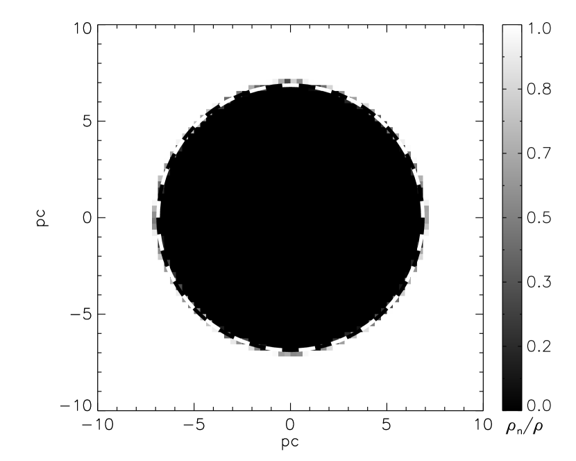
Figure 4.— Ratio of neutral to total density $\rho_{n}/\rho$ in an equatorial slice through our 3D computational domain in a simulation of an $R$ type ionization front without recombinations. The time shown is the same as that in Figure 3. The dashed line shows the analytically-computed front position.

4.2. R Type Ionization Fronts with Recombination

A next test of our code is in the case where there are still no motions, but recombinations do occur. Physically, this represents the next phase in the expansion of an R type ionization front, when the recombination rate becomes competitive with the photoionization rate, but before the excess pressure in the ionized gas causes the HII region to begin hydrodynamically expanding. If the recombination coefficient $\alpha^{(B)}$ is constant, this problem has an analytic solution: at time $t$, the radius of the ionization front is

$$r_{i}=r_{s}\left(1-e^{-t/t_{\rm rec}}\right)^{1/3},$$ (36)

where

$$r_{s}=\left(\frac{3s\mu_{H}^{2}}{4\pi\alpha^{(B)}\rho^{2}}\right)^{1/3}$$ (37)

is the Strömgren radius and

$$t_{\rm rec}=\frac{\mu_{H}}{\alpha^{(B)}\rho}$$ (38)

is the recombination time scale for the gas. At early times this solution matches the case of powerlaw expansion discussed in § 4.1, but as times $t\raisebox{-2.15277pt}{$\>\stackrel{{\scriptstyle\textstyle>}}{{\sim}}\>$}t_{\rm rec}$ the ionization front slows down due to recombinations. At times $t\gg t_{\rm rec}$, the front radius approaches $r_{s}$ and the front velocity drops to zero.

For any realistic cooling curve, for which the heaitng and cooling rates depend on the density, radiation flux, and the ionization state, there will be some small temperature variation in time and space within the HII region, so $\alpha^{(B)}$ will not be exactly constant and the analytic solution will not apply exactly. To enable us to compare with the analytic solution as well as possible, and therefore to make the strongest possible evaluation of the code, for the purposes of this test we set $\alpha^{(B)}=2.59\times 10^{-13}$ cm^-3 s^-1 independent of temperature.

We run this test using the same initial conditions and resolution as in § 4.1, which give $r_{s}=5.0$ pc and $t_{\rm rec}=1.2$ kyr for our chosen value of $\alpha^{(B)}$. For this test, we again disable the MHD update step in our code, but allow the entire radiation module to operate normally. We run for $10^{11}$ s ($3.17$ kyr), which is more than $2t_{\rm rec}$. Figure 5 shows the position of the ionization front versus time, computed as in § 4.1, and Figure 6 shows the radial profile of the neutral density at a time of $10^{11}$ s. As we found in § 4.1, the ionization front is entirely confined to a radial extent of a single cell, so the front is as spherical as possible given our Cartesian grid. The accuracy of the front position is $\sim 1\%$, better than a single cell.

Figure 5.— Ionization front radius $r_{i}$ versus time $t$ (upper panel), and error in simulated $r_{i}$ relative to the analytic value versus time (lower panel) in a simulation of an R type ionization front with recombinations. The upper panel shows the radius computed in the simulation (plus signs), the analytically computed radius (solid line), and the analytic prediction for the radius if there are no recombinations (dashed line). We define the ionization front radius as the mean radius of the centers of all cells for which $0.01<\rho_{n}/\rho<0.99$. The error is defined as $|r_{\rm sim}-r_{\rm analyt}|/r_{\rm analyt}$, where $r_{\rm sim}$ is the radius found in the simulation and $r_{\rm analyt}$ is the analytically computed value.

Figure 6.— Ratio of neutral to total density $\rho_{n}/\rho$ versus radius $r$ for a subsample of cells in our computational domain at a time of $10^{11}$ s ($3.17$ kyr) in a simulation of an R type ionization front with recombinations. The scale bar above the location of the ionization front shows a range of $\pm(\sqrt{3}/2)\Delta x$ about the analytically computed radius of the ionization front at this time.

4.3. D Type Ionization Fronts

The tests described in § 4.1 and § 4.2 demonstrate that our radiation module produces correct results on its own, and the tests in Gardiner & Stone (2005, 2006) show that the MHD module works well. However, we must also test how the two modules work together. We therefore consider the problem of the hydrodynamic evolution of a uniform neutral medium with initial density $\rho_{n}$ and temperature $T_{n}$ within which there is an ionizing source. This problem has a well-known solution. At early times there is an R type ionization front: the source ionizes the gas out to a radius $r_{i}\approx r_{s}$, and heats it to $T_{i}\approx 6400$ K, but the gas does not move and the ionization front is not preceeded by a shock. However, the ionized region is overpressured relative to the surrounding gas, and it expands on a sound crossing time scale, $t_{s}\equiv r_{s}/c_{i}$, where $c_{i}\approx 8\times 10^{5}$ cm s^-1 is the sound speed in the ionized gas. As it expands, it sweeps up a dense shell of neutral material, forming a D type ionization front. The expansion is subsonic with respect to the ionized gas, so the ionized region has an almost uniform density and temperature. Ionization balance requires that this density vary as $\rho_{i}\propto r_{i}^{-3/2}$, so the shell is driven outward by a pressure $p=\rho_{i}c_{i}^{2}\propto r_{i}^{-3/2}$. In the limit where the pressure in the ionized region that is driving the shell greatly exceeds the thermal pressure in the ambient medium, and the neutral mass in the shell greatly exceeds the mass within the ionized region, conservation of momentum for the shell implies that after a time $t$ it expands to a radius (Spitzer, 1978)

$$r_{\rm sh}=r_{s}\left(1+\frac{7t}{4t_{s}}\right)^{4/7}.$$ (39)

The thickness of the shell relative to its radius is of order $(c_{n}/v_{\rm sh})^{2}$, where $c_{n}$ is the isothermal sound speed in the neutral gas and $v_{\rm sh}=c_{i}[1+(7/4)t/t_{s}]^{-3/7}$ is the velocity of the shell. As with the analytic solution for the R type ionization front, this strictly applies only if the ionized gas sound speed $c_{i}$ is constant. For a realistic cooling curve, we expect this to be nearly but not perfectly true.

We run simulations with an initial density $\rho=2.34\times 10^{-22}$ g cm^-3, temperature $T=11$ K, and an ionizing source of luminosity $s=4.0\times 10^{46}$ s^-1. The source is placed at the center of a box running from $-10$ pc to $10$ pc in every direction. For these values of $\rho$ and $s$, and assuming an ionized region temperature of roughly $8.0\times 10^{3}$ K, we have $r_{s}=0.5$ pc and $t_{s}=0.061$ Myr. We expect that the similarity solution will apply for times $1\ll t/t_{s}\ll 1000$. The lower limit on the time is imposed by the requirement that the mass in the swept-up shell be much larger than the mass in the interior of the HII region, and the upper time limit comes from the requirement that the pressure in the HII region greatly exceed the ambient pressure, or equivalently that the thickness of the shell be much smaller than its radius. We run all our tests for 1 Myr, or $16.3t_{s}$.

4.3.1 Comparison to the Analytic Solution

We begin with simulations at resolutions of $64^{3}$, $128^{3}$, and $256^{3}$, using a factor $f=4$ for our heating time step constraint (i.e. we allow the internal energy of a cell to change by up to a factor of 4 between hydrodynamic updates.) Figure 7 shows the radial distribution of densities, temperatures, neutral fractions, and isothermal sound speeds in the gas in the simulations after 1 Myr. As we expect, the density and temperature in the ionized region are almost constant. The density peaks at the position of the overdense shell, but the shell is spread over a few cells, so its width decreases with resolution. This spreading is to be expected. The true physical thickness of the shell at this time should be roughly a percent of $r_{\rm sh}$, smaller than the size of a single computational cell. However, our code has some numerical viscosity, particularly for motions that are not aligned with the computational grid, and this spreads shocks over $\sim 3$ cells. As Figure 8 shows, despite this spreading the front remains round at each resolution.

Figure 7.— Hydrogen number density, temperature, neutral fraction, and isothermal sound speed versus radius for a selection of computational cells in our simulation of a D type ionization front, at resolutions of $64^{3}$ (left column), $128^{3}$ (middle column), and $256^{3}$ (right column). We show only a subsample of the gridpoints to minimize clutter and file size. The points are plotted at a time of $1$ Myr ($17.7t_{s}$) after the start of the simulation. The scale bars in the uppermost panels indicate a range of $\pm 3(\sqrt{3}/2)\Delta x$ about the analytically computed radius of the dense shell at this time, to indicate a width of 3 cells, about the expected width of a shock due to numerical viscosity.

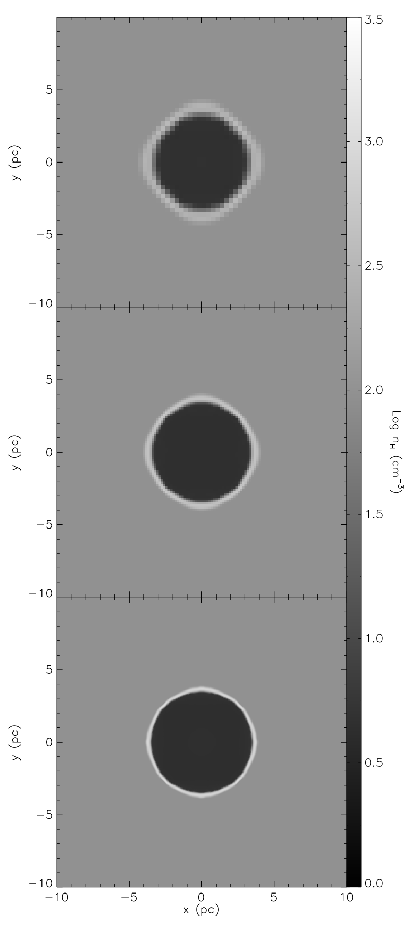
Figure 8.— Slice through the $xy$ plane showing log of hydrogen number density in a simulation of a D type ionization front 1 Myr ($17.7t_{s}$) after the start of the simulation, at a resolution of $64^{3}$ (top panel), $128^{3}$ (middle panel), and $256^{3}$ (bottom panel). The slices in the $xz$ and $yz$ planes are nearly identical.

We next compute the radius of the dense shell as a function of time in our simulation. We do this by identifying all the cells whose densities are at least 10% larger than the initial density, and then taking the average of their radii. Using an overdensity cutoff different from $10\%$ modifies the results in detail, but not qualitatively. We compare this measurement to the analytic solution in Figure 9. As the plot shows, the radius of our simulated shell matches the analytically computed radius at late times quite well in all the runs. The error is always smaller than cell in size, which is the best that can be expected using a Cartesian grid with finite numerical viscosity. This error is $\sim 3\%$ of the analytically computed radius at the lowest resolution and less than $1\%$ at the highest resolution. The error generally decreases with time, both because the ratio of the radius to a cell size is increasing, and because the analytic solution is becoming a better and better approximation as time increases.

Figure 9.— Radius of the dense shell around an HII region verus time (top panel), computed analytically (solid line) and by simulations at resolutions of $64^{3}$ (plus signs), $128^{3}$ (asterisks), and $256^{3}$ (diamonds). We also show the difference between the simulated and analytically-computed shell radii, $r_{\rm sim}$ and $r_{\rm analyt}$, normalized to the analytic radius (middle panel) and normalized to the size of a computational cell (bottom panel).

4.3.2 Heating Time Step Convergence Tests

We have shown that our method can match the analytic solution for the propogation of a D type ionization front with a heating time step constraint of $f=4$, meaning that we allow the pressure in a cell to change by at most a factor of 4 between hydrodynamic updates. However, we would like to explore a range of heating time step constraints to determine if the accuracy of the solution is affected by the choice of $f$. We therefore re-run our $128^{3}$ simulation with $f=2$, $f=10$, and $f=100$ to see if the quality of the solution changes significantly. The choice $f=100$ corresponds to essentially no constraint on the hydrodynamic time step other than the ordinary Courant condition. We wish to use as large a value of $f$ as possible, because that will minimize the computational cost by enabling us to take fewer of the more expensive MHD updates per radiation update. Of course if $f$ is too large then the cost of the radiation update will dominate the total computation cost, and there will be no additional advantage in increasing $f$. Where exactly this crossover occurs depends on the number of processors and the geometry of the ionization front.

Figure 10 shows the radius of the shell versus time as computed in our simulations with varying values of $f$, and as computed analytically. The results show that the radius approaches the analytic solution somewhat fall all $f$, but that the error is larger and the convergence slower for larger values of $f$. This suggests that numerical methods in which the temperature change between hydrodynamic updates is unconstrained (e.g. Dale et al., 2005; Mellema et al., 2005, 2006) or is limited only to values of $f\gg 10$ (e.g. Mac Low et al., 2006) may produce quantitatively incorrect results for the expansion rates of D type ionization fronts, although the error is likely to be only a few cells. This problem may not affect methods that implicitly update the hydrodynamics and the radiation together (e.g. Miniati & Colella, 2006), rather than in an operator split fashion, but we are unaware of any such methods for ionizing radiation transport as opposed to local heating and cooling functions.

Note, however, that even with large $f$ the error does decrease in time. This result is easy to understand intuitively. Once the front is well into the D type phase, the Courant time step is set by the sound speed in the ionized region, which is roughly constant. As the front sweeps up more material and slows down, the rate at which gas is heated from the inital temperature to the ionized temperature decreases, so, on average, the fractional change in cell temperature per fixed Courant time step is a decreasing function of time. Thus, the error one makes by allowing a large change in gas temperature per Courant time step decreases with time. This means that codes with unconstrained temperature changes per hydrodynamic update are likely to be most inaccurate at early times when fronts are moving at speeds close to the ionized sound speed, and are most accurate at late times when fronts move slowly.

Figure 10.— Radius of the dense shell around an HII region verus time (upper panel), computed analytically (solid line) and by simulations at a resolution of $128^{3}$, with $f=2$ (plus signs), $f=4$ (asterisks), $f=10$ (diamonds), and $f=100$ (triangles). We also show the fractional error in the position of the shell relative to the similarity solution (lower panel), defined as $|r_{\rm sim}-r_{\rm analyt}|/r_{\rm analyt}$, where $r_{\rm sim}$ is the simulated radius and $r_{\rm analyt}$ is the analytically computed radius.

4.3.3 Ray Rotation

To demonstrate why it is necessary to rotate the orientation of the rays in our calculation regularly, we repeat our $128^{3}$, $f=4$ test calculation without ever rotating the rays. The mean radial positions of the dense shell and the ionization front are essentially the same in the two calculations, but the shape of the ionization front is significantly different. Figure 11 shows the neutral fraction in slices through the simulations without and with ray rotation after 1 Myr of evolution. With rotation of the rays, as shown in the lower panel, the ionization front boundary is smooth and round. Without rotation, as shown in the upper panel, there are projections of partially neutral gas several cells into the ionized region, and the front boundary is much less smooth. If one is interested in studying instabilities or similar phenomena at the ionization front boundary, the presence of these fingers of neutral gas is potentially problematic, since they may serve as seeds for instability.

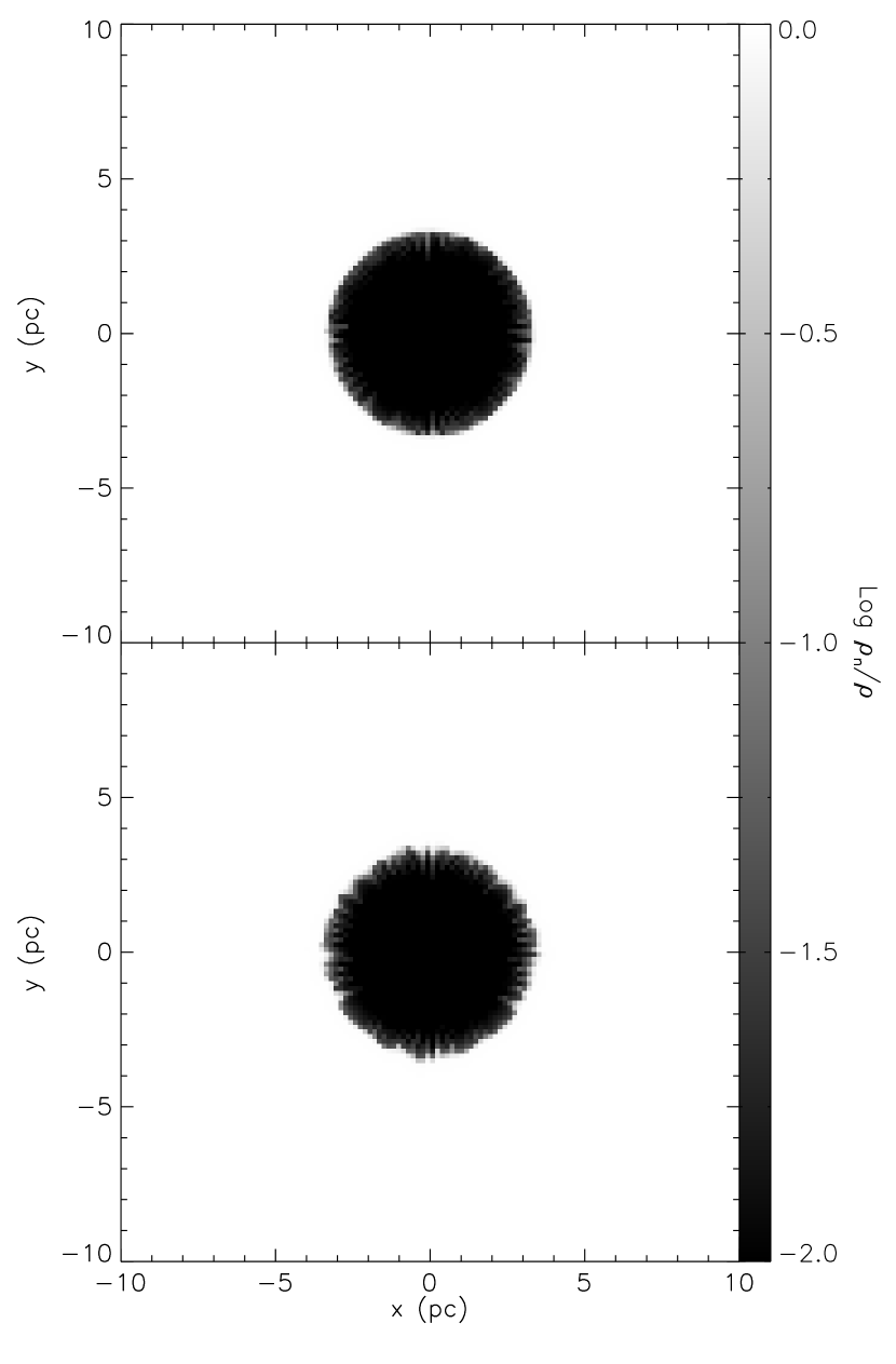
Figure 11.— Slice through the $xy$ plane showing log of the ratio of neutral density to total density in a simulation of a D type ionization front 1 Myr ($17.7t_{s}$) after the start of the simulation, with (upper panel) and withpout (lower panel) rotation of the rays.

These projections are caused by differences in ionization rate for cells at the same radius due to discretization in angle. When the orientation of the rays is constant over long times, small differences in ionization rate at different angles can build up to produce the finger-like structures shown in the figure. One could reduce the discretization error by using a more refined ray tree, for example by requiring that the solid angle subtended by a cell always be at least four times as large as the solid angle corresponding to a single ray, rather than twice as large as we require. However, this is potentially expensive, since every factor $f$ increase in the angular resolution multiplies the time required to compute the photoionization rate by a factor of $f^{2}$, and the photoionization rate is computed during every radiation iteration. It is also overkill, since the angular disretization errors only build up over many time steps. Rotating the rays at intervals of 5 hydrodynamic time steps, as we have done for the simulation shown in the lower panel of Figure 11, eliminates or vastly reduces the occurence of neutral gas fingers in the ionized region. The computational cost of rebuilding the ray tree every 5 hydrodynamic time steps is completely negligible and, for parallel calculations, requires no additional inter-processor communication.

4.3.4 Ionization Front Cooling

We next explore the question of cooling in cells with mixed ionization states. As discussed in § 3.3, we set the molecular cooling rate $\Lambda_{\rm KI}=\Gamma_{\rm KI}=0$ in cells where the ionization fraction is between $1\%$ and $99\%$ in order to prevent excessive cooling due to numerical mixing of ionized and neutral gas. To demonstrate why this is necessary, we repeat our simulation of a D type ionization front with $f=4$ with cooling allowed in all cells regardless of ionization fraction.

Figure 12 shows the result. The run where all cells can cool lags the analytic solution even at early times, and the error does not decrease with time. The error at 1 Myr of evolution is roughly 14%, which is far larger than a single cell; the error in the slope of the of the $r_{\rm sh}$ versus $t$ curve at 1 Myr is 10%. In contrast, the error with mixed-ionization cooling disabled is $1.5\%$, which corresponds roughly to the center-to-corner distance of a single cell. The slope of the curve differs from the analytic value by less than 1%.

Figure 12.— Radius of the dense shell around an HII region verus time (upper panel), computed analytically (solid line) and by simulations at a resolution with cooling in mixed-ionization cell disabled (plus signs) and enabled (asterisks). We also show the fractional error in the position of the shell relative to the similarity solution (lower panel), defined as $|r_{\rm sim}-r_{\rm analyt}|/r_{\rm analyt}$, where $r_{\rm sim}$ is the simulated radius and $r_{\rm analyt}$ is the analytically computed radius. For comparison, we also show the fractional error corresponding to a difference of $(\sqrt{3}/2)\Delta x$ (dashed line), the distance from the center of a computational cell to its corner.

The lag is a result of numerical mixing at the ionization front coupled with strong molecular cooling. To demonstrate this, we plot in Figure 13 both the total cooling rate $\mathcal{L}=\Lambda_{\rm KI}n_{H}^{2}+\Lambda_{\rm rec}n_{e}n_{H^{+}}+\Lambda_{\rm ion-ff}n_{e}n_{H^{+}}$ (panel a) and the molecular cooling rate $\Lambda_{\rm KI}n_{H}^{2}$ (panel b) as a function of position from our run with cooling in mixed cells allowed, at a time of 1 Myr. As the plot shows, with cooling allowed in mixed cells, the energy loss rate from cells at the ionization front is much larger than that from cells either inside or outside the front.

One might think this is to be expected, since the cells at the ionization front are the ones furthest out of equilibrium, and are the places where much of the energy from ionizing photons is deposited. However, 91% of the cooling in the region with an ionization fraction larger than $1\%$ comes from molecular cooling rather than from recombination or forbidden line cooling, the processes that should dominate in ionized regions. Molecular cooling dominates even if we consider only much more strongly ionized regions. Only if we limit our attention to gas where the ionization fraction is greater than $74\%$ do we find that molecular processes provide less than 50% of the total cooling rate. That molecular cooling is the dominant cooling process even in gas that is up to 74% ionized is a clear sign that the cooling rate is being artificially enhanced by numerical smearing of the ionization front, since for a real ionization front there should be no molecules to cool in regions that are significantly ionized.

This suggests that simulations can only compute the correct expansion rate for HII regions if they suppress the effects of numerical mixing at the ionization front. This may explain why some numerical simulations without this precaution produce results that lag the true solution significantly (e.g. Mac Low et al., 2006, figure 1) unless they have enough resolution to at least marginally resolve the ionization front (e.g. Arthur & Hoare, 2006), something that is not generally feasible in three dimensions. Note, however, that the strength of this effect depends on the existence of extremely rapid cooling processes for the non-ionized gas. If the chemistry is such that the neutral gas is not able to cool rapidly, the error will be much smaller. For example, with primordial cosmological chemistry the lag is much smaller because the neutral gas cooling is much less efficient (D. Whalen, 2006, private communication).

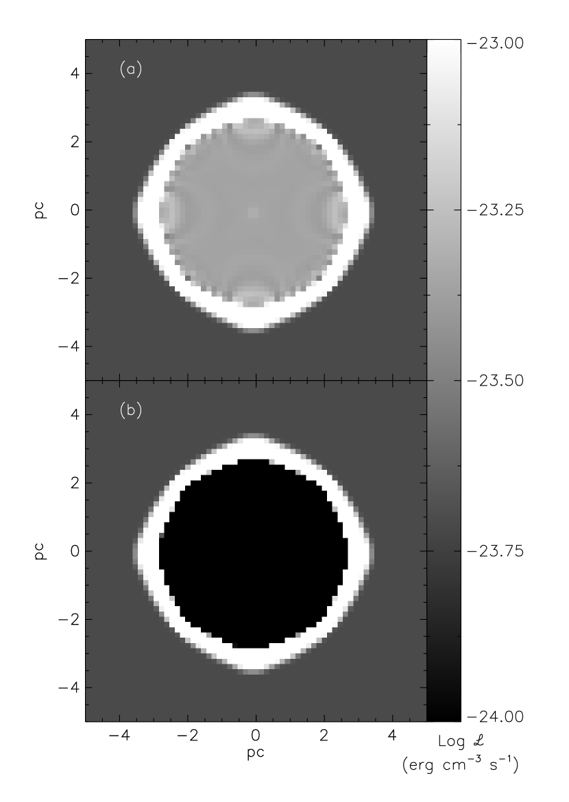
Figure 13.— Slice through the $xy$ plane showing the total cooling rate (panel a) and the cooling rate due to molecular processes alone (panel b). Note that, in order to make the cooling rate in the fully ionized region visible, we have selected a color scale that saturates in the rapidly cooling ionization front. The maximum cooling rate reaches $>10^{-21}$ erg cm^-3 s^-1.

An important point is that the evolution in the case with overcooling is qualitatively correct. There is an expanding, spherical HII region driving a dense shell of swept-up material, and following a radius versus time curve that resembles the correct solution. It is only when one quantitatively checks the numerical method against an analytic solution that the problem becomes clear. This highlights the importance of performing quantitative comparisons of numerical and analytic results.

5. HII Region Evolution in Uniform Magnetized Media

Now that we have determined the constraints our numerical method must obey from tests against analytic solutions in the hydrodynamic case, in this section we demonstrate our method in the simplest magnetohydrodynamic case. Several authors have considred the structure of magnetized ionization fronts in the past. However, these treatments have been limited to mathematically rigorous but one-dimensional analyses (e.g. Redman et al., 1998; Williams et al., 2000; Williams & Dyson, 2001) or to simple, quasi-empirical models (e.g. Carlqvist et al., 2003; Ryutov et al., 2005) in more dimensions. Bertoldi (1989) gives an analytic model for the implosion of a spherical magnetized gas clump exposed to an external ionizing source, but his solution is limited to that case. To date, there has been no detailed simulation of the evolution of an HII region driven by a point source expanding into a magnetized medium in three dimensions.

We consider a neutral medium with initially uniform density $\rho_{n}$ and isothermal sound speed $c_{n}$, threaded by a magnetic field $\mathbf{B}_{n}$ oriented in the $x$ direction. We place a source of constant ionizing luminosity $s$ at the origin that begins radiating at time $t=0$. We restrict ourselves to the case most relevant to ionizing sources in magnetized molecular clouds, in which the thermal pressure in ionized gas at the initial density greatly exceeds the magnetic pressure, which in turn greatly exceeds the thermal pressure in neutral gas at the initial density. Thus, $c_{i}\gg v_{A}\gg c_{n}$, where $v_{A}$ is the Alfven speed in the neutral gas and $c_{i}$ is the ionized gas sound speed.

5.1. Analytic Evaluation

We can sketch out an approximate evolutionary scenario for this configuration using simple analytic estimates. At times $t\raisebox{-2.15277pt}{$\>\stackrel{{\scriptstyle\textstyle<}}{{\sim}}\>$}t_{s}$, the gas has not yet had time to move in response to photoionization heating. Since photons do not feel the magnetic field, the evolution should be identical to that of a non-magnetized R type ionization front. At $t\sim t_{s}$, the ionized gas begins to expand due to its high thermal pressure. Since by assumption $c_{i}\gg v_{A}$, the magnetic field in the gas is initially unable to resist this expansion. Thus, as in the non-magnetic case, a D type ionization front forms, gas moves radially outward, and a spherical dense shell forms. Ionization balance requires that when the shell bouding the HII region reaches a radius $r_{\rm sh}$, the gas that remains in its interior and is not in the shell wall must have started within a distance

$$r_{0}=\sqrt{r_{s}r_{\rm sh}}=r_{s}\left(1+\frac{7t}{4t_{s}}\right)^{2/7}$$ (40)

of the ionizing source. Since the magnetic field is frozen into the gas, the magnetic flux passing through the interior of the ionized region is therefore

$$\Phi_{i}=\pi B_{n}r_{0}^{2}=\pi B_{n}r_{s}^{2}\left(1+\frac{7t}{4t_{s}}\right)^{4/7},$$ (41)

where $B_{n}$ is the magnitude of the magnetic field in the neutral gas outside the shell. In contrast, the total flux passing through the ionized region and the dense shell combined is simply the initial flux that passed through a circle of radius $r_{\rm sh}$,

$$\Phi_{\rm sh}=\pi B_{n}r_{\rm sh}^{2}=\pi B_{n}r_{s}^{2}\left(1+\frac{7t}{4t_{s}}\right)^{8/7}.$$ (42)

Since the magnetic flux through the HII region interior rises as $t^{4/7}$ at late times, while the total flux through the HII region interior and the dense shell varies as $t^{8/7}$, the fraction of magnetic field lines passing through the HII region that pass through the shell interior must decline with time as $t^{-4/7}$. Physically, this occurs because magnetic field lines are being dragged with the gas out of the HII region interior and concentrated in the dense shell.

As time progresses, the magnetic field changes the evolution in two ways. First, magnetic pressure and tension oppose the expansion of the shell perpendicular to the magnetic field, causing it to deform and become aspherical. This effect should become significant when magnetic pressure is comparable to thermal pressure in the ionized gas, i.e. when $\rho_{n}v_{A}^{2}\sim\rho_{i}c_{i}^{2}$. Since $\rho_{i}\approx(r_{\rm sh}/r_{s})^{-3/2}\rho_{n}$ before magnetic effects are significant, we should see significant deformation of the HII region when it reaches a radius of order $r_{\rm sh}\approx(c_{i}/v_{A})^{4/3}r_{s}$, and the shell velocity is $v_{\rm sh}\approx v_{A}$. Second, magnetic pressure in the swept-up shell will limit compression in the shock perpendicular to the magnetic field to a factor of order $v_{\rm sh}/v_{A}$. This will make the shell thinner along the field and thicker perpendicular to it, an effect that will become noticable when $v_{\rm sh}\sim v_{A}$. Thus, we expect both magnetic effects to become significant when the region has expanded to a radius of roughly

$$r_{m}\equiv\left(\frac{c_{i}}{v_{A}}\right)^{4/3}r_{s},$$ (43)

where we have defined the magnetic critical radius $r_{m}$ for the HII region. Assuming $r_{m}\gg r_{s}$, this happens at roughly a time

$$t_{m}\equiv\frac{4}{7}\left(\frac{c_{i}}{v_{A}}\right)^{7/3}t_{s}$$ (44)

after the start of the evolution.

The evolution will then enter a new stage in which the thermal pressure inside the ionized region is small compared to the magnetic pressure, but both still greatly exceed the thermal pressure in the neutral gas. Since $|\mathbf{B}|^{2}\gg\rho_{i}c_{i}^{2}$, gas will be able to move only along field lines, and those field lines will be approximately straight. Since expansion is subsonic with respect to the ionized gas and we are concerned with times $\gg t_{s}$, the density in the ionized gas along each field line is constant. Along the field, gas motions are unrestricted and the evolution will be a normal D type ionization front as seen in non-magnetized gas. Perpendicular to the field, magnetic pressure effects become more and more dominant as time goes on. The ionized gas continues to escape along field lines, so the pressure driving expansion perpendicular to the field continues falling, which causes the front to slow and the density contrast to decrease perpendicular to the field. At the same time, everywhere that the magnetic field is at all oblique to the front, a slow mode will move into the neutral medium. This mode will remove magnetic support from the front by bending the field lines so that they become perpendicular to the shock (Williams et al., 2000). This loss of magnetic support will cause the shell to transition from thick and magnetic pressure-dominated to thin and without much magnetic support over a larger and larger solid angle as time goes on, until only the circle exactly perpendicular to the initial magnetic field is not occupied by a dense shell.

5.2. Simulation

We simulate an initially neutral uniform medium with density $\rho_{n}=2.34\times 10^{-22}$ g cm^-3 ($n_{H}=100$ cm^-3) and temperature $T_{n}=11$ K, threaded by a magnetic field $\mathbf{B}=14.2\,\hat{\mathbf{x}}$ $\mu$G ($4.0\times 10^{-6}$ in the units we use in this paper). This gives an Alfven speed of 2.6 km s^-1 and a sound speed of 0.20 km s^-1 in the gas at the initial time. The computational domain runs from $-10$ pc to $10$ pc in every direction, and there is an ionizing source at the origin with luminosity $s=4.0\times 10^{46}$ s^-1, giving an initial Strömgren radius $r_{s}=0.5$ pc and sound crossing time $t_{s}=0.056$ Myr, assuming a sound speed $c_{i}=8.7$ km s^-1 in the ionized region. For these parameters the magnetic critical radius is $r_{m}=6.0r_{s}=2.5$ pc and the magnetic critical time is $t_{m}=9.4t_{s}=0.53$ Myr. The simulation uses a resolution of $256^{3}$ cells and a heating/cooling time step constraint of $f=4$. We run the simulation for a time of $3t_{m}=1.58$ Myr.

5.2.1 Structure at $t\ll t_{m}$

Figures 14 and 15 show slices through the computational domain at a time of $t\approx t_{m}/3=0.177$ Myr. As expected, the HII region almost spherical, although there is already a slight asymmetry visible. The outer boundary of the dense shell is nearly perfectly round, and is at essentially the same radius as we would expect for a non-magnetized region at the same time. However, the shell is slightly thicker in the direction perpendicular to the field than in the direction along the field, due to magnetic pressure opposing compression. Also as expected, because magnetic field lines are being advected with the gas, the magnetic field inside the HII region is much weaker than the background field, and the magnetic field in the dense shell is much stronger than the background field.

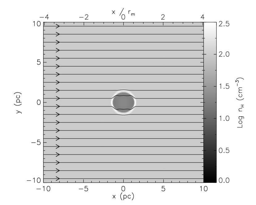
Figure 14.— Slice through the $xy$ plane showing log of hydrogen number density in a simulation of an ionization front expanding into a magnetized medium after a time of roughly $t_{m}/3=0.177$ Myr. The lines are magnetic field lines. The density of lines outside of the HII region corresponds to a magnetic field strength of $14.2$ $\mu$G.

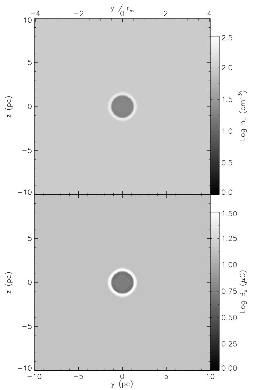
Figure 15.— Slices through the $yz$ plane showing log of hydrogen number density (upper panel) and log of magnetic field strength (lower panel) in a simulation of an ionization front expanding into a magnetized medium after a time of roughly $t_{m}/3=0.177$ Myr.

5.2.2 Structure at $t\sim t_{m}$

Figures 16 and 17 show the same slices as Figures 14 and 15 at a time $t\approx t_{m}=0.53$ Myr. As expected, the magnetic effects have now become pronounced. The inner, ionized region is strongly prolate, so that it is roughly a factor of 2 longer along the field than perpendicular to it. Along the field, the dense shell is still only a few cells thick, the same as in the non-magnetic case, but in the directions perpendicular to the field its thickness is not much smaller than its radius, again as we expect. However, the outer edge of the expanding shell is still not too far from spherical, and in the direction along the field its radius is close to $r_{m}$, the radius we would expect were there no field present.

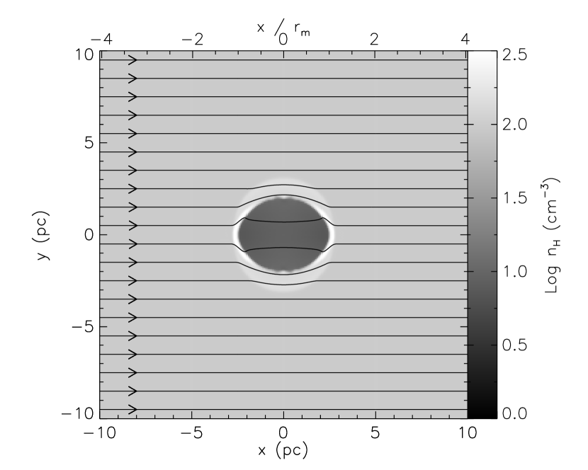
Figure 16.— Slice through the $xy$ plane showing log of hydrogen number density in a simulation of an ionization front expanding into a magnetized medium after a time of roughly $t_{m}=0.53$ Myr. The lines are magnetic field lines. The density of lines outside of the HII region corresponds to a magnetic field strength of $14.2$ $\mu$G.

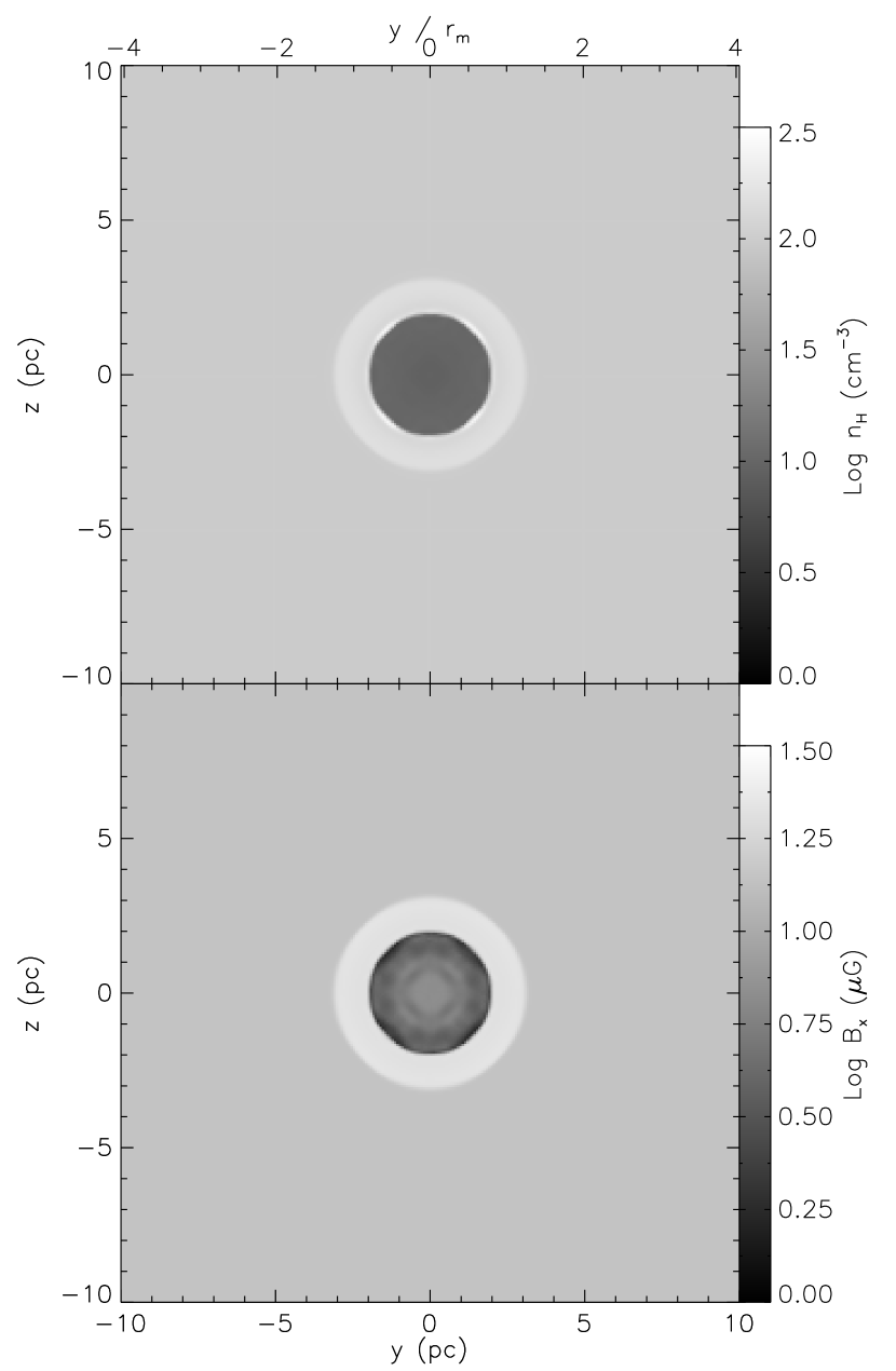
Figure 17.— Slices through the $yz$ plane showing log of hydrogen number density (upper panel) and log of magnetic field strength (lower panel) in a simulation of an ionization front expanding into a magnetized medium after a time of roughly $t_{m}=0.53$ Myr.

Interestingly, the shell extends somewhat further in the direction across the field than in the direction along it, so the outer radius of the swept up shell in the $y$ and $z$ directions is noticably larger than $r_{m}$. This is likely because at $t=t_{m}$ the expansion speed is comparable to the Alfven speed, and is slower than the fast magnetosonic speed. Across the field, signals from the shell can propogate by fast magnetosonic waves more rapidly than the shell can expand along the field. This creates a density disturbance, carried by the fast mode, ahead of the radius that the shell would have reached had there been no magnetic field. Since fast waves cannot propogate parallel to the magnetic field, the leading edge of the disturbance has advanced less in the $x$ direction than in the $y$ or $z$ directions.

5.2.3 Structure at $t\gg t_{m}$

Figures 18 and 19 show the simulation at our final time slice, $t=1.58\mbox{ Myr}=3t_{m}$. In the evolution after time $t_{m}$, the inner ionized region becomes more prolate, expanding more rapidly along the field than perpendicular to it. Along the field, in the $x$ direction, there continues to be dense shell of swept up material.

In the $y$ and $z$ directions, perpendicular to the field lines, the thick shell of gas bounded between the ionization front and the fast mode front, has also continued to expand. However, its overdensity is decreasing, and at this time is only $120$ cm^-3, so it is within $20\%$ of the background density, and smaller than the density at time $t_{m}$. The shell expansion velocity perpendicular to the field lines is much smaller than the Alfven speed in the neutral gas, and is comparable to the sound speed, so the leading edge of the shell is no longer a shock. Instead, the shell is just a small overdensity that is gradually relaxing away.

The boundary between the neutral and ionized regions in the $y$ and $z$ directions appears to be somewhat corrugated, but this may well be a numerical artifact, particularly since Figure 19 shows that the structure at the ionization front is aligned with the computational grid. It may be that for ionization fronts that are nearly static, as this one is due to magnetic confinement, rebuilding the ray tree once every five time steps is insufficient to prevent the growth of structures.

In between the $x$ direction and the $y$ direction, there is a region where the field is oblique relative to the ionization front. As predicted by Williams et al. (2000), this region shows two types of behavior depending on how close the field is to being parallel or perpendicular to the front. Closer to the $x$ direction, the field been bent so it is close to perpendicular to the front, and a dense shell bounded has formed at the ionization front. Closer to the $y$ direction, the field is not bent and enters the front at an oblique angle, and there is no shock or dense shell. The solid angle over which a dense shell exists appears to be increasing in time.

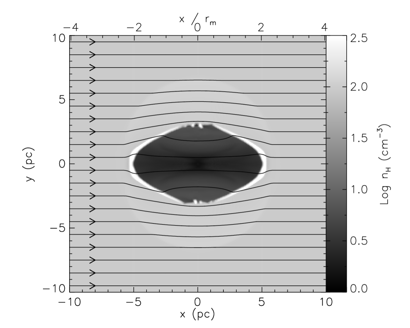
Figure 18.— Slice through the $xy$ plane showing log of hydrogen number density in a simulation of an ionization front expanding into a magnetized medium after $1.58$ Myr ($3t_{m}$). The lines are magnetic field lines. The density of lines outside of the HII region corresponds to a magnetic field strength of $14.2$ $\mu$G.

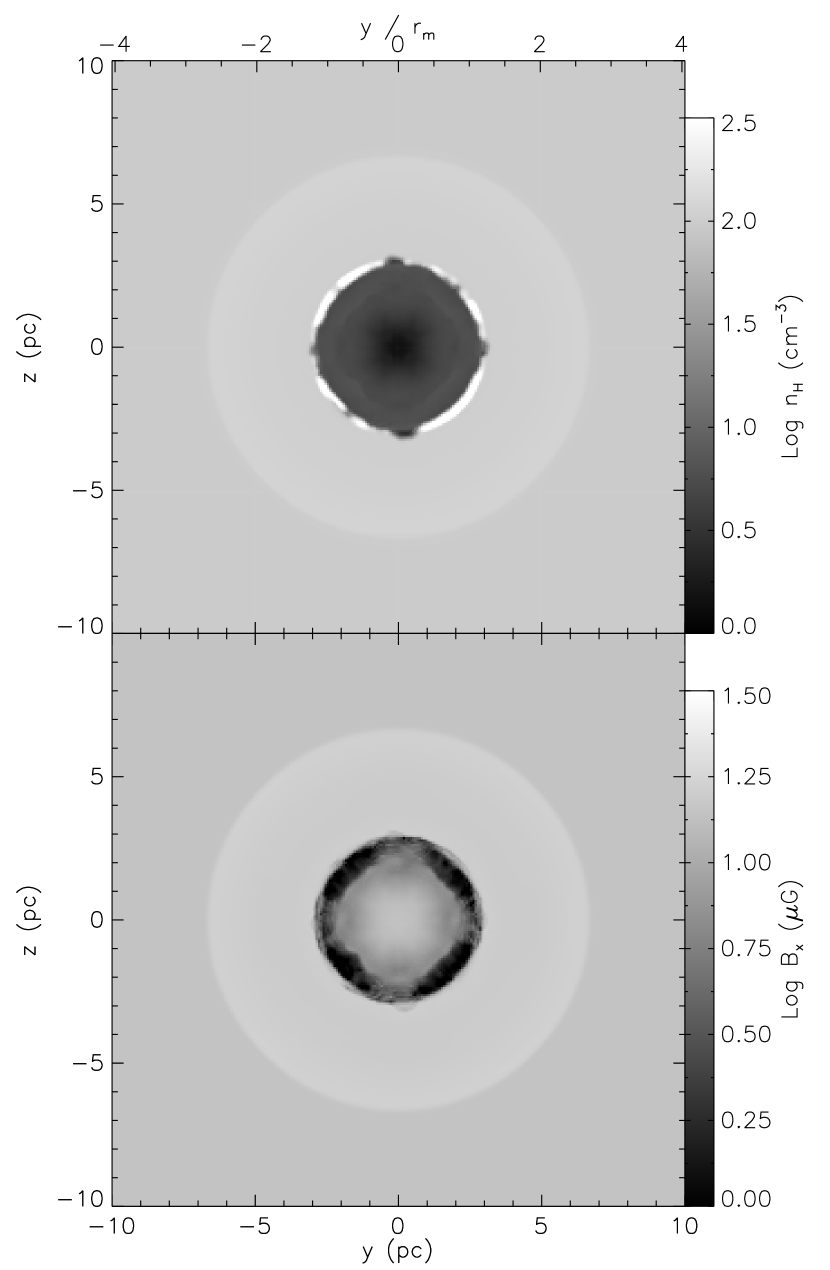
Figure 19.— Slices through the $yz$ plane showing log of hydrogen number density (upper panel) and log of magnetic field strength (lower panel) in a simulation of an ionization front expanding into a magnetized medium after $1.58$ Myr ($3t_{m}$).

While expansion of the ionized region perpendicular to the field has slowed, the expansion velocity along the field lines is actually larger or about the same as it was at time $t_{m}$. To understand the origin of this effect, consider the jump conditions that govern the expansion of the dense shell in the $x$ direction at late times, when the expansion is strongly subsonic with respect to the ionized gas, but the thermal pressure in the ionized gas is still much greater than the thermal pressure in the neutral gas. In the rest frame of the shell, this means that ram pressure of neutral gas flowing into the shell must balance the thermal pressure of ionized gas downstream from it. Thus, $\rho_{n}v_{\rm sh}^{2}\propto\rho_{i}c_{i}^{2}$, so the shell expansion velocity obeys $v_{\rm sh}\propto c_{i}\sqrt{\rho_{i}/\rho_{n}}$. Thus far our analysis could apply just as well to a non-magnetized HII region. The difference that the magnetic field makes is that it greatly reduces the expansion rate of the ionized region in two directions. This prevents the density from dropping as fast as in the hydrodynamic case, which keeps the expansion velocity larger at later times.

However, while the decline in ionized gas density and pressure is slower than in the hydrodynamic case, since gas continues to flow out of the ionzied region along field lines into the end caps, the pressure inside the HII region is always decreasing after time $t_{m}$. By $3\,t_{m}$, the HII region is in the limit where the magnetic pressure inside the ionization front is higher than the thermal pressure. As a result, the field lines have begun to straighten out inside the ionized region, so they are kinked only at the dense end caps. The magnetic energy density inside the ionized region is actually larger than at time $t_{m}$, since for $t\raisebox{-2.15277pt}{$\>\stackrel{{\scriptstyle\textstyle>}}{{\sim}}\>$}t_{m}$ field lines that were pushed into the dense shell start to move back into the ionized region interior.

6. Discussion and Conclusion

We have demonstrated an algorithm for computing the evolution of magnetized molecular gases subjected to internal sources of ionizing radiation, which is potentially applicable to molecular clouds. In testing our algorithm, we have discovered three conditions that are likely to apply to ionizing radiation hydrodynamic and magnetohydrodynamic codes in general. First, to achieve maximum accuracy the update time step must be limited so that the temperature in cells does not change by more than a factor of $f<10$ between hydrodynamic or magnetohydrodynamic updates. Larger values of $f$ produce small but significant errors in the expansion rates of D type ionization fronts. Second, when using a ray-tracing approach to compute the ionizing radiative transfer, one should rotate the orientation of the rays periodically to avoid a build-up of errors caused by the discretization of angles around the ionizing source. Failure to obey this conditions results in fronts that should be spherical developing aspherical features, and in more complex calculations this could potentially seed instabilities. Third, and most significantly, one must avoid overcooling caused by numerical smearing of the ionization front. This can be handled most easily by suppressing cooling in cells with mixed ionization fractions. Failure to obey this condition leads to an unphysical loss of energy from expanding HII regions that causes them to lag analytic solutions by tens of percent. A calculation that satisfies these three constraints can reproduce the analytic solution for the expansion of a D type ionization front to an accuracy of a percent for at least $\sim 20$ ionized sound-crossing times.

Using our algorithm, we report the first three-dimensional simulations of the expansion of an HII region into a magnetized gas. We show that the presence of a magnetic field distorts the HII region, and greatly reduces the strength of the shock and the density contrast in directions perpendicular to the magnetic field. This leads to the formation of an HII region which is bounded by a dense shell of swept-up gas along the field, but not perpendicular to it. The absence of a dense shell over much of the solid angle means that, in the presence of strong, ordered magnetic fields, HII regions may not be able to collect and compress as much gas as one might expect from purely hydrodynamic estimates. This may reduce the efficiency of triggered star formation from HII regions.

References

- Abel & Wandelt (2002) Abel, T. & Wandelt, B. D. 2002, MNRAS, 330, L53
- Arthur & Hoare (2006) Arthur, S. J. & Hoare, M. G. 2006, ApJS, in press, astro-ph/0511035
- Bertoldi (1989) Bertoldi, F. 1989, ApJ, 346, 735
- Bertoldi & Draine (1996) Bertoldi, F. & Draine, B. T. 1996, ApJ, 458, 222
- Blitz et al. (2005) Blitz, L., Fukui, Y., Kawamura, A., Leroy, A., Mizuno, N., & Rosolowsky, E. 2005, Protostars and Planets V, in press, astro-ph/0602600
- Carlqvist et al. (2003) Carlqvist, P., Gahm, G. F., & Kristen, H. 2003, A&A, 403, 399
- Crutcher (1999) Crutcher, R. M. 1999, ApJ, 520, 706
- Crutcher (2005) Crutcher, R. M. 2005, in IAU Symposium 227: Massive Star Birth: A Crossroads of Astrophysics, ed. R. Cesaroni, M. Felli, E. Churchwell, & M. Walmsley, 98–107
- Dale et al. (2005) Dale, J. E., Bonnell, I. A., Clarke, C. J., & Bate, M. R. 2005, MNRAS, 358, 291
- Garcia-Segura (1997) Garcia-Segura, G. 1997, ApJ, 489, L189+
- Garcia-Segura & Franco (1996) Garcia-Segura, G. & Franco, J. 1996, ApJ, 469, 171
- García-Segura & López (2000) García-Segura, G. & López, J. A. 2000, ApJ, 544, 336
- Gardiner & Stone (2005) Gardiner, T. A. & Stone, J. M. 2005, JCP, 205, 509
- Gardiner & Stone (2006) —. 2006, JCP, submitted
- Górski et al. (2005) Górski, K. M., Hivon, E., Banday, A. J., Wandelt, B. D., Hansen, F. K., Reinecke, M., & Bartelmann, M. 2005, ApJ, 622, 759
- Heiles & Crutcher (2005) Heiles, C. & Crutcher, M. 2005, Magnetic Fields in Diffuse HI and Molecular Clouds (Berlin: Springer), in press, astro-ph/0501550
- Henney (2006) Henney, W. J. 2006, in Diffuse Matter from Star Forming Regions to Active Galaxies, ed. T. W. Hartquist, J. M. Pittard, & S. A. E. G. Falle, in press, astro-ph/0602626
- Hosokawa & Inutsuka (2005) Hosokawa, T. & Inutsuka, S.-i. 2005, ApJ, 623, 917
- Koyama & Inutsuka (2002) Koyama, H. & Inutsuka, S. 2002, ApJ, 564, L97
- Krumholz et al. (2006) Krumholz, M. R., Matzner, C. D., & McKee, C. F. 2006, ApJ, 653, 361
- Krumholz & McKee (2005) Krumholz, M. R. & McKee, C. F. 2005, ApJ, 630, 250
- Mac Low et al. (2006) Mac Low, M.-M., Toraskar, J., Oishi, J. S., & Abel, T. 2006, ApJ, submitted, astro-ph/0605501
- Matzner (2002) Matzner, C. D. 2002, ApJ, 566, 302
- McKee & Williams (1997) McKee, C. F. & Williams, J. P. 1997, ApJ, 476, 144
- Mellema et al. (2005) Mellema, G., Arthur, S. J., Henney, W. J., Iliev, I. T., & Shapiro, P. R. 2005, ApJ, submitted, astro-ph/0512554
- Mellema et al. (2006) Mellema, G., Iliev, I. T., Alvarez, M. A., & Shapiro, P. R. 2006, New Astronomy, 11, 374
- Miniati & Colella (2006) Miniati, F. & Colella, P. 2006, JCP, submitted, astro-ph/0601519
- Osterbrock (1989) Osterbrock, D. E. 1989, Astrophysics of gaseous nebulae and active galactic nuclei (University Science Books)
- Redman et al. (1998) Redman, M. P., Williams, R. J. R., Dyson, J. E., Hartquist, T. W., & Fernandez, B. R. 1998, A&A, 331, 1099
- Rijkhorst et al. (2005) Rijkhorst, E.-J., Plewa, T., Dubey, A., & Mellema, G. 2005, A&A, submitted, astro-ph/0505213
- Ritzerveld (2005) Ritzerveld, J. 2005, A&A, 439, L23
- Ryutov et al. (2005) Ryutov, D. D., Kane, J. O., Mizuta, A., Pound, M. W., & Remington, B. A. 2005, Ap&SS, 298, 183
- Sofia & Meyer (2001) Sofia, U. J. & Meyer, D. M. 2001, ApJ, 554, L221
- Spitzer (1978) Spitzer, L. 1978, Physical Processes in the Interstellar Medium (New York: Wiley-Interscience)
- Tenorio-Tagle et al. (1986) Tenorio-Tagle, G., Bodenheimer, P., Lin, D. N. C., & Noriega-Crespo, A. 1986, MNRAS, 221, 635
- Whalen & Norman (2006) Whalen, D. & Norman, M. L. 2006, ApJS, 162, 281
- Williams & McKee (1997) Williams, J. P. & McKee, C. F. 1997, ApJ, 476, 166
- Williams & Dyson (2001) Williams, R. J. R. & Dyson, J. E. 2001, MNRAS, 325, 293
- Williams et al. (2000) Williams, R. J. R., Dyson, J. E., & Hartquist, T. W. 2000, MNRAS, 314, 315
- Zuckerman & Evans (1974) Zuckerman, B. & Evans, N. J. 1974, ApJ, 192, L149