Point source power in three-year Wilkinson Microwave Anisotropy Probe data

Abstract

Using a set of multifrequency cross-spectra computed from the three year WMAP sky maps, we fit for the unresolved point source contribution. For a white noise power spectrum, we find a Q-band amplitude of $A=0.011\pm 0.001$ $\mu$K² sr (antenna temperature), significantly smaller than the value of $0.017\pm 0.002$ $\mu$K² sr used to correct the spectra in the WMAP release. Modifying the point source correction in this way largely resolves the discrepancy Eriksen et al. (2006) found between the WMAP V- and W-band power spectra. Correcting the co-added WMAP spectrum for both the low-$\ell$ power excess due to a sub-optimal likelihood approximation—also reported by Eriksen et al. (2006)—and the high-$\ell$ power deficit due to over-subtracted point sources—presented in this letter—we find that the net effect in terms of cosmological parameters is a $\sim 0.7\sigma$ shift in $n_{\textrm{s}}$ to larger values: For the combination of WMAP, BOOMERanG and Acbar data, we find $n_{\textrm{s}}=0.969\pm 0.016$, lowering the significance of $n_{\textrm{s}}\neq 1$ from $\sim 2.7\sigma$ to $\sim 2.0\sigma$.

1 Introduction

The results of Wilkinson Microwave Anisotropy Probe have made an inestimable impact on the science of cosmology, highlighted by the very recent release of the three year data: maps, power spectra, and consequent cosmological analysis (Jarosik et al., 2006; Page et al., 2006; Hinshaw et al., 2006; Spergel et al., 2006). Precisely because these results play so prominent a role, it is important to check and recheck their consistency.

Recently Eriksen et al. (2006) reanalyzed the WMAP three year temperature sky maps, and noted two discrepancies in the WMAP power spectrum analysis. On large angular scales there is a small power excess in the WMAP spectrum (5–10% at $\ell\lesssim 50$), primarily due to a problem with the likelihood approximation used by the WMAP team. On small angular scales, an unexplained systematic difference between the V- and W-band spectra (few percent at $\ell\gtrsim 300$) was found. In this Letter, we suggest this second discrepancy is at least partially due to an excessive point source correction in the WMAP power spectrum.

2 Data

The WMAP temperature data (Hinshaw et al., 2006) are provided as ten sky maps observed at five frequencies between 23 and 94 GHz, pixelized using the HEALPix scheme with 3 million ($\sim$ 7′-size) pixels per map. Here we consider the Q-band (41 GHz), V-band (61 GHz), and W-band (94 GHz) channels since these have the least galactic foreground contamination, but only V- and W-bands for the cosmological parameter analysis.

We account for the (assumed circularly symmetric) beam profile of each channel independently, adopting the Kp2 sky cut as our mask. This excludes 15.3% of the sky including all resolved point sources. To deal with contamination outside the mask, we simply use the foreground template corrected maps provided on the LAMBDA website. The noise is modeled as uncorrelated, non-uniform, and Gaussian with an RMS given by $\sigma_{0,i}/\sqrt{N_{\textrm{\scriptsize obs},i}(p)}$. Here $\sigma_{0,i}$ is the noise per observation for channel $i$, and $N_{\textrm{\scriptsize obs},i}(p)$ is the number of observations in pixel $p$.

3 Methods

3.1 Power spectrum estimation

We estimate power spectra with the pseudo-$C_{\ell}$ MASTER method (Hivon et al., 2002), which decouples the mode correlations in a noise-corrected raw quadratic estimate of the power spectrum computed on the partial sky. Following Hinshaw et al. (2003), we include only cross-correlations between channels in our power spectrum estimates.

Considering each of three years, three bands, and the number of differencing assemblies per band (two for Q-/V- and four for W-band), 276 individual cross-spectra are available for analysis. Each of these is computed to ${\ell_{\rm max}=1024}$. The V- and W-band spectra have been verified against spectra provided by the WMAP team, but the Q-band spectra (computed the same way) were not available for comparison. For the point source amplitude analysis, we bin the power spectra into ten bins ($\ell=2$–$101$, $102$–$201$,…, $902$–$1001$) in order to increase the signal-to-noise ratio and decrease the number of bins (and thus the computation time). The corresponding error bars are computed using a Fisher approximation and similarly binned.

3.2 Point source amplitude estimation

For our main result, we marginalize over the CMB power and estimate a single amplitude for the point source spectrum by the method we discuss below. We also compute the amplitude in $\ell$-bins, but for brevity omit the details, which are similar. We model the ensemble averaged cross-spectra as the sum of the two components, $\langle C^{\mathbf{i}}_{l}\rangle=C^{{\mathbf{i}},\rm CMB}_{l}+C^{{\mathbf{i}},\rm src}_{l}$, showing explicitly the contribution from each part of the signal. Here the multipole bin is denoted by $l$ and the cross-correlation pair by ${\mathbf{i}}={(i_{1})(i_{2})}=$ (W1yr1)(W2yr3), (Q1yr2)(V1yr2), etc. No auto-power spectra are included, so noise subtraction is unnecessary. We marginalize over the CMB spectrum, which we denote by $C_{l}^{\rm{CMB}}$. The window functions for each differencing assembly pair are ${\mathbf{w}}=\{w^{\mathbf{i}}_{ll^{\prime}}\}$, which we later consider in terms of a matrix. The contribution to a cross-spectrum from the CMB signal is thus $C^{{\mathbf{i}},\rm CMB}_{l}=\sum_{l^{\prime}}w^{\mathbf{i}}_{ll^{\prime}}C^{\rm{CMB}}_{l^{\prime}}$ (in thermodynamic temperature units). The spectra in this application are already beam-deconvolved, so the window functions $w^{\mathbf{i}}_{ll^{\prime}}=\delta_{ll^{\prime}}$ are trivial. We denote the amplitude of the unresolved point source power spectrum by $A$. This amplitude relates to the cross-spectra via the frequency and shape dependence vector ${\mathbf{S}}=\{S^{\mathbf{i}}_{l}\}$,

$$C_{l}^{{\mathbf{i}},\rm src} = AS^{\mathbf{i}}_{l}$$

$$S^{\mathbf{i}}_{l} = w^{\mathbf{i}}_{ll}\ \left(\frac{\nu_{i_{1}}}{\nu_{0}}\right)^{\beta}\ K\left(x(\nu_{i_{1}})\right)\left(\frac{\nu_{i_{2}}}{\nu_{0}}\right)^{\beta}\ K\left(x(\nu_{i_{2}})\right)$$

$$K(x) = \frac{\left(\exp(x)-1\right)^{2}}{x^{2}\exp(x)}.$$ (1)

Here the cross-spectrum ${\mathbf{i}}$ has channels at $\nu_{i_{1}}$ and $\nu_{i_{2}}$, and $x(\nu)={h\nu}/{k_{B}T_{\rm CMB}}$. The units of $A$ are antenna temperature squared times solid angle and the function $K(x)$ converts from antenna temperature to thermodynamic temperature. Thus, we assume that the radio sources are spatially uncorrelated (and therefore have a white noise spectrum) and have a power-law frequency dependence using antenna temperature units. Note that well-resolved point sources have already been masked from the maps before the evaluation of the cross-spectra, and $A$ therefore represents unresolved sources only. However, we may only directly measure the frequency dependence for the resolved sources. For these, Bennett et al. (2003) found $\beta=-2.0$, and following Hinshaw et al. (2003, 2006) we take the same even for the unresolved sources. We choose $\nu_{0}=40.7$ GHz (Q-band) as our reference frequency.

We organize the binned cross-spectra $C^{\mathbf{i}}_{l}$ into a data vector ${\mathbf{D}}=\{C^{\mathbf{i}}_{l}\}$. We use a Gaussian model for the likelihood $\mathcal{L}$ of the power spectrum, appropriate at high $\ell$:

$$\mathcal{L}\propto\exp\left\{-\frac{1}{2}\left[{\mathbf{D}}-\langle{\mathbf{D}}\rangle\right]^{{\dagger}}{\mathbf{\Sigma}}^{-1}\left[{\mathbf{D}}-\langle{\mathbf{D}}\rangle\right])\right\},$$ (2)

where the covariance ${\mathbf{\Sigma}}=\langle({\mathbf{D}}-\langle{\mathbf{D}}\rangle)({\mathbf{D}}-\langle{\mathbf{D}}\rangle)^{{\dagger}}\rangle$ can be written as ${\mathbf{\Sigma}}=\{\Sigma^{{\mathbf{ii^{\prime}}}}_{ll^{\prime}}\}$. Here we assume the covariance is diagonal both in multipole and cross-spectrum. An appendix of Huffenberger et al. (2004) derives an unbiased estimator for this type of problem, generalizing the point source treatment of Hinshaw et al. (2003). Here the estimators are equivalent, and result in a linear estimate for $A$, denoted $\bar{A}$, and its covariance $\Sigma^{A}$:

$$\bar{A} \equiv ({\mathbf{S}}^{{\dagger}}\mathbf{F}{\mathbf{S}})^{-1}{\mathbf{S}}^{{\dagger}}\mathbf{F}{\mathbf{D}}$$

$$\Sigma^{A} \equiv ({\mathbf{S}}^{{\dagger}}\mathbf{F}{\mathbf{S}})^{-1},$$ (3)

where we have defined the auxiliary matrix

$$\mathbf{F} \equiv {\mathbf{\Sigma}}^{-1}-{\mathbf{\Sigma}}^{-1}{\mathbf{w}}\left({\mathbf{w}}^{{\dagger}}{\mathbf{\Sigma}}^{-1}{\mathbf{w}}\right)^{-1}{\mathbf{w}}^{{\dagger}}{\mathbf{\Sigma}}^{-1}.$$

In this notation, we consider ${\mathbf{D}}$ and ${\mathbf{S}}$ as column vectors with a single index ${\mathbf{i}}l$, and ${\mathbf{w}}$ as a matrix with indices ${\mathbf{i}}l$ and $l^{\prime}$. Matrices ${\mathbf{\Sigma}}$ and $\mathbf{F}$ have indices ${\mathbf{i}}l$ and ${\mathbf{i}}^{\prime}l^{\prime}$. This estimator marginalizes out the CMB, a conservative treatment which assumes nothing but the frequency dependence. To compute the amplitude in bins, we redefine $A$ as ${\mathbf{A}}$, a vector of the amplitudes, with $C^{{\mathbf{i}},\rm src}_{l}=({\mathbf{A}}\cdot{\mathbf{S}})^{{\mathbf{i}}}_{l}$, modifying ${\mathbf{S}}$ for each component to lend power only to appropriate multipole bins.

4 Results

4.1 Point source spectrum amplitude

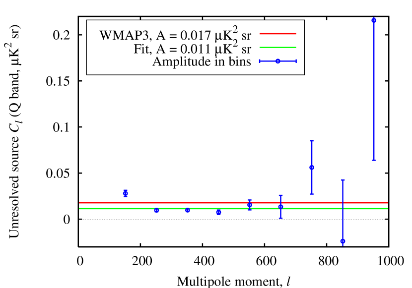
Figure 1: The point source power spectrum, fit from WMAP Q-, V-, and W- bands. The lowest $\ell$ bin is not plotted, because the error bars span the entire range of the plot, and it has little statistical influence. The 1-parameter fit for a flat spectral shape is also shown, as well as the point source amplitude from Hinshaw et al. (2006).

Using the method described in the previous section, we find a point source amplitude of $A=0.011\pm 0.001$ $\mu$K² sr, significantly less than the WMAP value of $A=0.017\pm 0.002$ $\mu$K² sr (Hinshaw et al., 2006). Computing the spectrum in bins (Figure 1), we see that the source power spectrum is best measured at $100<\ell<600$. To evaluate goodness-of-fit, we compute $\chi^{2}=\sum_{l\textrm{\scriptsize\ bin}}(A_{l}-A)^{2}/\sigma^{2}_{l}=36.6$ for 9 degrees of freedom. All of the discrepancy in our fit arises from a single high bin at $\ell=102$–$201$, which has $\Delta\chi^{2}=27.2$. This bin is so different that we suspect that it is not detecting point source power alone, but perhaps some residual foreground. We leave a rigorous investigation of this anomalous bin to later work, leaving it in our analysis here. If we were to exclude it, the other nine bins are consistent with a flat power spectrum at $A=0.011$ $\mu$K² sr—with $\chi^{2}=9.4$ for 8 remaining degrees of freedom—though they would prefer a somewhat smaller value for $A$. For the WMAP amplitude, we measure $\chi^{2}=86.5$ for 9 degrees of freedom. This large discrepancy is puzzling because our method should be equivalent to the WMAP method.

4.2 Angular CMB power spectrum

The net effect of the lower unresolved point source amplitude on the co-added WMAP CMB power spectrum may be computed in terms of a weighted average of corrections for individual cross-spectra (V$\times$V, V$\times$W, and W$\times$W, respectively). Following the construction of WMAP’s spectrum, for $\ell<500$ the correction is given by a uniform average over the 137 individual cross-spectrum corrections; for $\ell\geq 500$ it is given as an inverse noise weighted average (Hinshaw et al., 2006). In this Letter we approximate the latter with the inverse variance of the power spectrum coefficients computed from 2500 simulations for each cross-spectrum individually, but do not account for correlations between different cross-spectra.

The net power spectrum correction is shown in Figure 2. We show the Q-band spectra, corrected by each point source amplitude, in the top panel of Figure 3, and compare the V- and W-band spectra in the bottom panel.

One of two issues pointed out by Eriksen et al. (2006) was a discrepancy between the V- and W-bands at $\ell\gtrsim 250$ significant at about $3\sigma$. This is seen by comparing the two red curves in the bottom panel of Figure 3. However, applying the lower point source correction raises the V-band spectrum by 10–$50\,\mu\textrm{K}^{2}$ in this range but the W-band by only a few $\mu\textrm{K}^{2}$. Effectively, about $20\,\mu\textrm{K}^{2}$ of the previous $65\,\mu\textrm{K}^{2}$ average difference is thus removed, reducing the significance of the difference from 3 to $2\sigma$, compared to 2500 simulations. A small difference is still present, and may warrant further investigation, but is no longer striking. This gives us confidence that our point source correction is the more consistent than the WMAP value.

4.3 Cosmological parameters

To assess the impact of this new high-$\ell$ correction on cosmological parameters, we repeat the analysis described by Eriksen et al. (2006) using the CosmoMC package (Lewis & Bridle, 2002, which also gives the parameter definitions) and a modified version of the WMAP likelihood code (Hinshaw et al., 2006). First, at $\ell\leq 30$ the WMAP likelihood is replaced with a Blackwell-Rao Gibbs sampling-based estimator (Jewell et al., 2004; Wandelt et al., 2004; Eriksen et al., 2004; Chu et al., 2005), and second, the bias correction shown in Figure 2 is added to the co-added WMAP spectrum. The results from these computations are summarized in Table 1.

As reported by Eriksen et al. (2006), the most notable effect of the low-$\ell$ estimator bias in the WMAP data release was a $\sim 0.4\sigma$ shift in $n_{\textrm{s}}$ to lower values, increasing the nominal significance of $n_{\textrm{s}}\neq 1$. In Table 1 we see that the over-estimated point source amplitude causes a similar effect by lowering the high-$\ell$ spectrum too much. Correcting for both of these effects, the spectral index is $n_{\textrm{s}}=0.969\pm 0.016$ for the combination of WMAP, BOOMERanG (Montroy et al., 2005; Piacentini et al., 2005; Jones et al., 2005) and Acbar (Kuo et al., 2004) data, or different from unity by only $\sim 2\sigma$. The marginalized distributions both with and without these corrections are shown in Figure 4. The other cosmological parameters change little. For reference, the best-fit (as opposed to marginalized) parameters for this case are $\{\Omega_{\textrm{b}}h^{2},\Omega_{\textrm{c}}h^{2},h,\tau,n_{\textrm{s}},\log(10^{10}A_{\textrm{s}})\}=(0.0225,0.108,0.732,0.919,0.967,3.05)$.

5 Conclusions

Using a combination of cross-spectra of maps from the Q-, V-, and W-bands of WMAP three year data, we fit for the amplitude of the power spectrum of unresolved point sources in Q-band, finding $A=0.011\pm 0.001$ $\mu$K² sr. This fit has significantly less power than the fit used to correct the WMAP final co-added power spectrum used for cosmological analysis.

We compute and apply the proper point source correction, noting the corrected V- and W-bands are more consistent than before. The improper point source correction conspires with a low-$\ell$ estimator bias to impart a spurious tilt to the WMAP temperature power spectrum. With the revised corrections, we find evidence for spectral index $n_{\textrm{s}}\neq 1$ at only $\sim 2\sigma$, while other parameters remain largely unchanged.

Table 1: Cosmological parameters

Parameter	WMAP	Low-$\ell$ and PS corrected
WMAP data only
$\Omega_{\textrm{b}}\,h^{2}$	$0.0222\pm 0.0007$	$0.0223\pm 0.0007$
$\Omega_{\textrm{m}}$	$0.241\pm 0.036$	$0.244\pm 0.035$
$\log(10^{10}A_{\textrm{s}})$	$3.019\pm 0.067$	$3.039\pm 0.068$
$h$	$0.731\pm 0.033$	$0.730\pm 0.032$
$n_{\textrm{s}}$	$0.954\pm 0.016$	$0.966\pm 0.016$
$\tau$	$0.090\pm 0.030$	$0.090\pm 0.030$
WMAP + Acbar + BOOMERanG
$\Omega_{\textrm{b}}\,h^{2}$	$0.0225\pm 0.0007$	$0.0225\pm 0.0007$
$\Omega_{\textrm{m}}$	$0.239\pm 0.031$	$0.240\pm 0.031$
$\log(10^{10}A_{\textrm{s}})$	$3.030\pm 0.064$	$3.045\pm 0.065$
$h$	$0.737\pm 0.029$	$0.738\pm 0.030$
$n_{\textrm{s}}$	$0.958\pm 0.016$	$0.969\pm 0.016$
$\tau$	$0.091\pm 0.030$	$0.091\pm 0.030$

Note. — Comparison of marginalized parameter results obtained from the WMAP likelihood (second column) and from the WMAP + Blackwell-Rao hybrid, applying the low-$\ell$ estimator and high-$\ell$ point source corrections (third column).

Figure 2: The net difference [$(C_{\ell}^{\rm new}-C_{\ell}^{\rm old})\ell(\ell+1)/2\pi$] in the final co-added WMAP spectrum due to the new and smaller point source amplitude. The sharp break at $\ell=500$ is due to different weighting schemes, and the smaller fluctuations at high $\ell$’s are due to a finite number of Monte Carlo simulations for noise estimation.

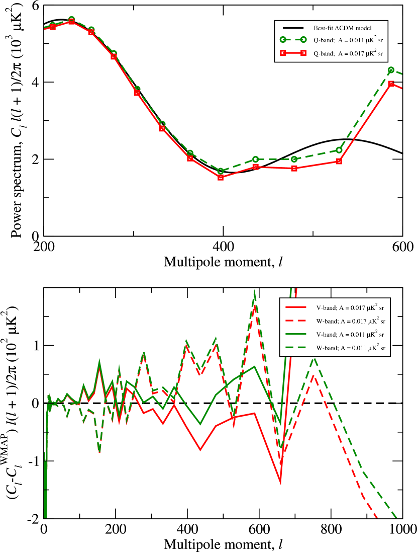
Figure 3: The impact on the Q-, V-, and W-band power spectra of the revised point source correction. The top panel shows the Q-band power spectrum with the WMAP point source correction (red) and the correction in this work (green dashed), plotted with the WMAP best-fit $\Lambda$CDM spectrum. Particularly at $\ell<400$ where noise is lower, this highlights the point source over-subtraction using the WMAP correction. The bottom panel shows the V-band (solid) and W-band (dashed) power spectra minus the co-added WMAP temperature spectrum (Hinshaw et al., 2006), computed with the WMAP point source correction (red) and the correction in this work (green). The V- and W- bands are internally more consistent with the revised source correction.

Figure 4: Marginalized posterior distributions for the spectral index $n_{\textrm{s}}$ computed with the combination of WMAP, BOOMERanG and Acbar data, both with the WMAP likelihood code as provided (dashed) and after applying a low-$\ell$ estimator correction and a high-$\ell$ point source correction (solid).

References

- Bennett et al. (2003) Bennett, C. L., et al. 2003, ApJS, 148, 97
- Chu et al. (2005) Chu, M.,et al. 2005, Phys. Rev. D, 71, 103002
- Eriksen et al. (2004) Eriksen, H. K., et al. 2004, ApJS, 155, 227
- Eriksen et al. (2006) Eriksen, H. K., et al. 2006, ApJ, submitted, [astro-ph/0606088]
- Finkbeiner et al. (1999) Finkbeiner D.P., Davis M., & Schlegel D.J. 1999, ApJ, 524, 867
- Finkbeiner (2003) Finkbeiner, D. P. 2003, ApJS, 146, 407
- Górski et al. (2005) Górski, K. M., Hivon, E., Banday, A. J., Wandelt, B. D., Hansen, F. K., Reinecke, M., & Bartelmann, M. 2005, ApJ, 622, 759
- Hinshaw et al. (2003) Hinshaw, G., et al. 2003, ApJS, 148, 135
- Hinshaw et al. (2006) Hinshaw, G., et al. 2006, ApJ, submitted [astro-ph/0603451]
- Hivon et al. (2002) Hivon, E., Górski, K. M., Netterfield, C. B., Crill, B. P., Prunet, S., & Hansen, F. 2002, ApJ, 567, 2
- Huffenberger et al. (2004) Huffenberger, K. M., Seljak, U., & Makarov, A. 2004, Phys. Rev. D, 70, 063002
- Jarosik et al. (2006) Jarosik, N., et al. 2006, ApJ, submitted, [astro-ph/0603452]
- Jewell et al. (2004) Jewell, J., Levin, S., & Anderson, C. H. 2004, ApJ, 609, 1
- Jones et al. (2005) Jones, W. C., et al. 2005, ApJ, submitted, [astro-ph/0507494]
- Kuo et al. (2004) Kuo, C. L., et al. 2004, ApJ, 600, 32
- Lewis & Bridle (2002) Lewis, A., & Bridle, S. 2002, Phys. Rev. D, 66, 103511
- Montroy et al. (2005) Montroy, T. E., et al. 2005, ApJ, submitted, [astro-ph/0507514]
- Page et al. (2006) Page, L., et al. 2006, ApJ, submitted, [astro-ph/0603450]
- Piacentini et al. (2005) Piacentini, F, et al. 2005, ApJ, submitted [astro-ph/0507507]
- Spergel et al. (2006) Spergel, D. N., et al. 2006, ApJ, submitted, [astro-ph/0603449]
- Wandelt et al. (2004) Wandelt, B. D., Larson, D. L., & Lakshminarayanan, A. 2004, Phys. Rev. D, 70, 083511