The Tully–Fisher relation and its evolution with redshift in cosmological simulations of disc galaxy formation

Abstract

We present predictions on the evolution of the Tully–Fisher (TF) relation with redshift, based on cosmological N-body/hydrodynamical simulations of disc galaxy formation and evolution. The simulations invoke star formation and stellar feedback, chemical evolution with non-instantaneous recycling, metallicity dependent radiative cooling and effects of a meta-galactic UV field, including simplified radiative transfer. At $z=0$, the simulated and empirical TF relations are offset by about 0.4 magnitudes (1 $\sigma$) in the B and I bands. The origin of these offsets is somewhat unclear, but it may not necessarily be a problem of the simulations only.

As to evolution, we find a brightening of the TF relation between $z=0$ and $z=1$ of about 0.85 mag in rest–frame B band, with a non-evolving slope. The brightening we predict is intermediate between the (still quite discrepant) observational estimates.

This evolution is primarily a luminosity effect, while the stellar mass TF relation shows negligible evolution. The individual galaxies do gain stellar mass between $z=1$ and $z=0$, by a 50–100%; but they also correspondingly increase their characteristic circular speed. As a consequence, individually they mainly evolve along the stellar mass TF relation, while the relation as such does not show any significant evolution.

The TF relation and its redshift evolution in cosmological simulations

1 Introduction

The Tully–Fisher (TF) relation is a most important distance indicator, but also a key to understand the structure and evolution of disc galaxies. Its slope is a standard test–bench for cosmologically motivated galaxy formation models (Dalcanton, Spergel & Summers 1997; Mo, Mao & White 1998; Sommer–Larsen, Götz & Portinari 2003, henceforth SGP03) and its absolute luminosity level is also a crucial constraint, suggesting low stellar mass–to–light ratios and “bottom–light” Initial Mass Functions in disc galaxies (Portinari, Sommer–Larsen & Tantalo 2004; henceforth PST04).

Table 1: Overview of literature results on the evolution of the TF relation; we indicate its brightening as $\Delta M_{B}=M_{B}(V_{c},0)-M_{B}(V_{c},z)$. Then we report the redshift range and median redshift of the sample, the number of galaxies and the reference paper.

$\Delta M_{B}$	$z$ range	$<z>$	$N_{gal}$	reference
1.5	0.15–0.35	0.25	24	Rix et al. (1997)
1.5–2	0.25–0.45	0.35	12	Simard & Pritchet (1998)
0.4	0.1–1	0.5	16	Vogt et al. (1996, 1997)
0.2	0.2–1	0.5	$\sim$100	Vogt (1999)
1.1	0.5–1.5	0.9	22	Barden et al. (2003)
1.6 $z$	0.15–0.9	0.4	19 (field)	Milvang–Jensen et al. (2003)
$\sim 0.8^{a}$	0.05–1	0.45	$\sim 120$	Böhm et al. (2004),
(1.22 $z$)a				Böhm & Ziegler (2006)
0.3	revised analysis of Böhm et al. ’s data			Kannappan & Barton (2004)
1.0 $z$	0.1–1	0.33	89	Bamford et al. (2006)
1.3 $z$	0.19–0.74	0.39	14	Nakamura et al. (2006)
$\raisebox{-3.8pt}{$\;\stackrel{{\scriptstyle\textstyle>}}{{\sim}}\;$}0$	0.4–0.75	0.53	11 (non-disturbed)	Flores et al. (2006)

^a For the sake homogeneous comparison to other data, we report in this table the Böhm et al. results for constant TF slope,

although the authors favour a slope evolution scenario to interpret their data (see text).

In the last decade, the increasing amount of observational data at intermediate and high redshifts have allowed to study also the evolution of the TF relation, as well as of other galaxy scaling relations. However, there is as of yet no convergence on the results (see the summary in Table 1). Rix et al. (1997) and Simard & Pritchet (1998) argued for strong luminosity evolution of disc galaxies (1.5–2 mag in rest–frame B band) already at $z=0.3$. Conversely, Vogt et al. (1996, 1997) found at most moderate evolution ($\Delta M_{B}\raisebox{-3.8pt}{$\;\stackrel{{\scriptstyle\textstyle<}}{{\sim}}\;$}$0.4 mag) for a sample of about 16 spiral galaxies at a median redshift of $z\sim 0.5$. Later on, basing on a much larger sample of 100 galaxies between $0.2<z<1$, Vogt (1999) further reduced the estimated evolution to $\Delta M_{B}\raisebox{-3.8pt}{$\;\stackrel{{\scriptstyle\textstyle<}}{{\sim}}\;$}$0.2 mag, almost entirely driven by strong brightening of a few dwarf galaxies at $z>0.5$. Most recently, from the analysis of the DEEP1 Groth Strip survey, Vogt (2006) reports no evolution at all (within $\pm$0.3 mag) in the TF relation out to $z\sim$1, in the sense that all of the apparent evolution can be entirely accounted for by observational and selection effects. Other groups instead find, out to $z\sim$1, a brightening up to 1 mag or more (Rigopoulou et al. 2002; Barden et al. 2003; Milvang–Jensen et al. 2003; Böhm et al. 2004; Bamford, Aragón–Salamanca & Milvang–Jensen 2006; Nakamura et al. 2006). Significant brightening is also indicated by the line width – luminosity relation at even higher redshifts: van Starkenburg et al. (2006) report a 2 mag offset for 3 galaxies at $z\sim$1.5. However, at so early epochs, one major concern is how to interpret the kinematics of galaxies, which may not have settled onto a well developed rotation curve comparable to those of local spirals.

Limiting our discussion to galaxies up to $z\sim$1, the discrepancy between different results shows that these are plagued by observational difficulties and selection effects. Smith et al. (2004) observed a disc galaxy at $z\sim$0.8 in integral field spectroscopy, deducing for this one object a far more negligible brightening with respect to the local TF relation, than found by Barden et al. with long–slit spectroscopy; this highlights the difficulties of measuring the kinematics of high redshift galaxies. Kannappan & Barton (2004) further suggest that a significant contribution to the apparent evolution may be due to disturbed kinematics biasing the measurements of rotation velocities in high redshift samples, where kinematic anomalies are both more frequent (in the hierarchical clustering scenario) and more difficult to assess; kinematic disturbances might also contribute to the discrepancies between results obtained from selecting large undisturbed discs (e.g. the Vogt paper series) and from other less selective samples. Indeed recently, Flores et al. (2006) have used 3D integral field spectroscopy to recover the velocity field of disc galaxies at $z=0.4-0.75$ and showed that the intermediate redshift TF relation of undisturbed rotating discs shows much reduced scatter and evolution than a generic sample including perturbed or complex kinematics.

It seems therefore that the results on the TF evolution are still dominated by observational difficulties, selection effects and systematics. A recalibration of the zero–point of the local comparison TF relation by about 0.5 mag (Tully & Pierce 2000 vs. Pierce & Tully 1992; see Fig. 3a) adds further confusion to the issue.

As to the slope of the TF relation, within the large scatter of the high redshift samples the slope is not very well constrained directly so the “minimal assumption” is usually adopted of an evolution at constant slope, i.e. of a uniform luminosity offset. However, there are some indications that evolution might be mass dependent, and that sub–$L_{*}$ objects drive the brightening (Simard & Prichet 1998; Vogt 1999); differential mass evolution might partly explain the discrepancies between the results from different samples. In their recent VLT sample Böhm et al. (2004) and Böhm & Ziegler (2006) find a brightening of about 0.8 mag if a constant TF slope is imposed, but their data are better fit by a changing slope implying much stronger brightening for dwarf galaxies. Kannappan & Barton (2004) suggest though that this differential behaviour might be driven by kinematic anomalies, namely that the objects with stronger evolution are likely kinematically disturbed rather than genuinely brighter; comparing the Böhm et al. data to a low redshift sample with similar selection as the high redshift one, they revise the estimated TF evolution down to a modest $\Delta M_{B}$=0.3 mag, with no change in slope. Bamford et al. (2006) further point out that a spurious change in slope may be due to intrinsic coupling between scatter in rotation speed, TF residuals and limited magnitude range of the sample; also Weiner et al. (2006) find no slope evolution in a revised analysis of the Böhm et al. (2004) data. Finally, very recently Weiner et al. (2006), from a large sample of TKRS/GOODS galaxies with $z$=0.4–1.2, argue for an evolution in TF slope in the opposite sense, with brighter, massive galaxies fading more than low mass galaxies. The issue of slope evolution remains quite controversial.

However quantitatively significant the luminosity evolution of the TF relation, there is some evidence that it must be largely a luminosity dimming effect of the aging stellar populations, while in terms of the stellar mass there is hardly any offset, at fixed $V_{c}$, between the TF relation at $z=0$ and at $z=1$ (Conselice et al. 2005; Flores et al. 2006).

In this paper we present our predictions on the evolution of the TF relation with redshift, based on cosmological+hydrodynamical simulations of disc galaxy formation. In Section 2 we describe our simulations and their analysis. In Section 3 we discuss the theoretical TF relation at $z=0$ and the effects of numerical resolution and softening length on the results. In Section 4 we illustrate the evolution of the TF relation as predicted by our simulations. A special experiment with no infall of hot halo gas after $z=1$ is discussed in Section 5. Finally, Section 6 outlines our conclusions.

2 The simulations

The code used for the simulations is a significantly improved version of the TreeSPH code we used for our previous work on galaxy formation (SGP03). A similar version of the code has been used recently to simulate clusters of galaxies, and a detailed description can be found in Romeo et al. (2006). Here we briefly mention its main features and the upgrades over the previous version of SGP03 — see also Sommer-Larsen (2006).

1. The basic equations are integrated by incorporating the “conservative” entropy equation solving scheme of Springel & Hernquist (2002), which improves the numerical accuracy in lower resolution regions.

2. Cold high-density gas is turned into stars in a probabilistic way as described in SGP03. In a star-formation event a SPH particle is converted fully into a star particle. Non-instantaneous recycling of gas and heavy elements is described through probabilistic “decay” of star particles back to SPH particles as discussed by Lia et al. (2002a). In a decay event a star particle is converted fully into a SPH particle, so that the number of baryonic particles in the simulation is conserved.

3. Non-instantaneous chemical evolution tracing 10 elements (H, He, C, N, O, Mg, Si, S, Ca and Fe) has been incorporated in the code following Lia et al. (2002a,b); the algorithm includes supernovæ of type II and type Ia, and mass loss and chemical enrichment from stars of all masses. For the simulations presented in this paper, we adopt the Initial Mass Function (IMF) of Kroupa (1998), derived for field stars in the Solar Neighbouhood; this IMF well reproduces the chemo–photometric properties of the Milky Way (e.g. Boissier & Prantzos 1999) and is “bottom–light”, which aids in reproducing the luminosity level of the TF relation (PST04). Two experiments have been run with the Salpeter IMF for comparison.

4. Atomic radiative cooling is implemented, depending both on the metallicity of the gas (Sutherland & Dopita 1993) and on the meta–galactic UV field, modelled after Haardt & Madau (1996). Moreover, a simplified treatment of radiative transfer, switching off the UV field where the gas becomes optically thick to Lyman limit photons on scales of $\sim$ 1 kpc, is invoked.

5. Star-burst driven winds are incorporated in the simulations at early epochs, as strong early feedback is crucial to largely overcome the angular momentum problem (SGP03). A burst of star formation is modelled in the same way as in SGP03: when a star particle is formed, further self-propagating star formation is triggered in the surroundings; the energy from the resulting, correlated SNII explosions is released initially into the interstellar medium as thermal energy, and gas cooling is locally halted to reproduce the adiabatic super–shell expansion phase; a fraction of the supplied energy is subsequently converted (by the hydro code itself) into kinetic energy of the resulting expanding super–winds and/or shells. The super–shell expansion also drives the dispersion of the metals produced by type II supernovæ (while metals produced on longer timescales are restituted to the gaseous phase by the “decay” of the corresponding star particles, see point 2 above).

   At later epochs, only a fraction (typically, 20%) of the stars induce efficient feedback, and star formation is no longer self–propagating so that no strong starbursts are triggered by correlated SN explosions. This allows the smooth settling of the disc (see SGP03 for all details).

The galaxies were drawn and re-simulated from a $10h^{-1}$ Mpc box-length dark matter (DM)-only cosmological simulation, based on the “standard” flat $\Lambda$ Cold Dark Matter cosmological model ($h=0.65$, $\Omega_{0}=0.3$, $\sigma_{8}=1.0$); our choice of $h$ and $\sigma_{8}$ is slightly different from presently more popular values (0.7 and 0.9 respectively), but this has little impact on the Tully-Fisher locus (see § 3.2.4). When re-simulating with the hydro-code, baryonic particles were “added” to the original DM ones, which were split according to an adopted baryon fraction $f_{b}=0.15$. The gravity softening lengths were fixed in physical coordinates from $z$=6 to $z$=0 and in comoving coordinates at earlier times.

Our model galaxies are typically run with a resolution of $m_{SPH}=m_{*}=1.1\times 10^{6}$ $M_{\odot}$, $m_{DM}=6.5\times 10^{6}$ $M_{\odot}$ and $\epsilon_{SPH}=0.6$ kpc (“normal resolution” henceforth); a few cases were run at “lower resolution”, with $m_{SPH}=m_{*}=9\times 10^{6}$ $M_{\odot}$, $m_{DM}=5.2\times 10^{7}$ $M_{\odot}$ and a gravitational softening length $\epsilon_{SPH}=\epsilon_{*}=1.2$ kpc, and some more at “high resolution” with $m_{SPH}=m_{*}=1.4\times 10^{5}$ $M_{\odot}$ and $\epsilon_{SPH}=0.3$ kpc. These are the characteristics of “normal softening length” (ns) simulations. For smaller galaxies ($V_{c}\raisebox{-3.8pt}{$\;\stackrel{{\scriptstyle\textstyle<}}{{\sim}}\;$}$150 km/sec), we run some normal and high resolution simulations with “long softening length” (ls), where $\epsilon_{SPH}=1.2$ kpc and $\epsilon_{SPH}=0.6$ kpc respectively.

We show below that the predicted locus and evolution of the TF relation is largely robust to changes in the numerical resolution. Images of the simulated galaxies are available at http://www.tac.dk/$\sim$jslarsen.

Figure 1: Bulge–to–disc ratio of simulated galaxies; clockwise from top left panel: in B, I, K band and in the actual stellar mass profile. The size of the dots increases with the numerical resolution of the corresponding simulation; “pairs” of triangles with the same orientation, pointing upward or downward (and same colour, in the colour version of the figure) mark simulations of the same object (or cosmological halo) resimulated at two different resolution levels. Asterisks show simulations run in the “long softening” (ls) mode. Dotted circle: the special “no late infall” experiment discussed in Section 5; the solid circle encircles the corresponding “normal infall” simulation.

Figure 2: Disc scalelengths of simulated galaxies in B, I, K band and in the actual stellar mass profile. Symbols as in Fig. 1. The solid lines show linear fits to the disc scalelengths, including only simulated galaxies with a realistic (B/D)${}_{I}\leq 0.6$. In the I band panel (top right), the observational relation by Sommer–Larsen (2003; see also Sommer–Larsen & Dolgov 2001) is also shown for comparison.

2.1 The analysis

We determine the disc plane of a simulated galaxy from the direction of the angular momentum vector of the star particles around the center of mass of the system. Each star particle in the simulation represents a Single Stellar Population (SSP) of given age and metallicity, whose luminosity in various bands is straightforwardly computed from the SSPs of PST04 (see also Section 2.2 of Romeo, Portinari & Sommer–Larsen 2005). Hence we compute the surface brightness profile of each galaxy on the disc plane; a thickness of 3 kpc is typically assumed for the disc stars, sometimes thinner or thicker (between 2 kpc and 5 kpc) as judged from visual inspection of the simulation. This limit ensures that 90–100% of the stars are included out to the very outskirts of the disc; in the inner disc regions, within 2 scalelengths where most of the stellar mass resides, the scaleheights are significantly smaller and more realistic (0.5–1 kpc for Milky Way–sized simulated galaxies; this is the vertical resolution achieved with the softening lengths typical of present–day fully cosmological simulations; cf. also Abadi et al. 2003; Governato et al. 2006). Since the Tully-Fisher is a global relation, the detailed vertical structure of our discs is not so crucial provided we make sure to include the bulk of the disc luminosity; indeed we verified that our results are robust with respect to the assumed thickness (e.g., 3 vs. 2 kpc). The large scaleheights do not have either a major impact on the effectiveness of the feedback process, which in our simulations is strong and crucial only in the early, pre-galactic starbursts, while it is much milder for the main part of bulge and disc formation. The limited resolution on the vertical structure of discs is thus not a concern for our basic picture of disc galaxy formation.

The one–dimensional radial profiles of stellar surface mass density and UBVRIJHK surface brightness are each decomposed into an exponential disc and a (de Vaucouleurs or exponential) bulge component by means of a Leverberg–Marquardt fitting algorithm (Press et al. 1992). Any bar component is included in the bulge and not treated separately. The fit is performed over the radial extent of the simulated discs as judged by visual inspection; typical disc radii range from 8–10 kpc for small galaxies, to 12–15 kpc (sometimes out to 20 kpc) for larger ones. The decomposition is in any case quite robust to the assumed disc edge. The decomposition with an exponential bulge profile provides better fits in general, so we will discuss this case only in the following. Assuming a de Vaucouleur bulge obviously results in larger bulge–to–disc (B/D) ratios but, although the central disc brightness is correspondingly lower, neither the derived disc scalelengths nor our results on circular velocities and the TF relations, discussed below, are much affected.

Fig. 1 and Fig. 2 show the B/D ratios (with exponential bulge component) and the disc scalelengths respectively, obtained for the stellar mass density profiles and the BIK surface brightness profiles of our galaxies. As expected, B/D ratios systematically increase going from blue to red bands, and to the actual stellar mass profile. Notice though that we also obtain a few bulgeless objects — although some of the apparent “pure discs” in B band are no longer such when the decomposition is performed in redder bands, or in the stellar mass profile. On the contrary, the disc scalelengths do not differ significantly in the different bands or going from the light distribution to the actual stellar mass one. Some of the simulated galaxies with large B/D ratios correspondingly display long scalelengths for the remaining (quite small) disc component; but a proper comparison to observations should consider only simulations with realistic B/D ratios for late–type galaxies. In Fig. 2 the solid lines are least square fits to the scalelength—circular velocity relation of simulated galaxies, limited to galaxies with (B/D)${}_{I}\leq 0.6$ (corresponding to (B/D)${}_{B}\raisebox{-3.8pt}{$\;\stackrel{{\scriptstyle\textstyle<}}{{\sim}}\;$}0.4$). In the I band (top right panel), this is compared to the observed relation derived by Sommer–Larsen & Dolgov (2001) from the Mathewson sample (dashed line). Our scalelengths are close to the observed average at low masses and within a factor of 1.5 from the empirical relation for Milky Way–type galaxies ($V_{c}\sim 200$ km/sec); this is an improvement also on the results of SGP03 (their Fig. 8), since only for the largest circular speeds ($V_{c}\sim 300$ km/sec) we now find a factor–of–2 offset from observed scalelengths.

To compare properly to observational TF studies, the circular velocity $V_{c}$ of the system is measured at 2.2 disc scalelengths, by summing in quadrature the contribution of the exponential disc component and of the (spherically distributed) bulge and dark matter halo. As the angular momentum problem is not yet fully resolved (Fig. 2), the disc contribution is computed by “correcting” its actual scalelength to the one expected from the observed scalelength—$V_{c}$ relation (dashed line in Fig. 2). Namely we “redistribute” the mass of the disc component according to the empirically expected scalelength for that circular velocity. $V_{c}$ is estimated at 2.2 scalelengths and both quantities are adjusted to each other by iteration. The procedure is as outlined in Sommer–Larsen & Dolgov (2001) and the main purpose is to avoid overestimating $V_{c}$ by measuring it at too inner radii (due to the short scalelengths) where the rotation curve of simulated galaxies typically presents a significant peak due to strong matter concentration in the central regions. Adjusting the scalelength to the “observationally expected” one we make sure to measure $V_{2.2}$ far out enough that we skip the inner peak of the rotation curve and select regions where the circular velocity is only smoothly varying and representative of the global gravitational potential of the system. In fact, once the disc scalelength is adjusted around the actual observed values, the corresponding $V_{2.2}$ is quite robust to e.g. the B/D ratio, to whether the bulge is considered point–like or modelled with an extended spherical symmetry, and so on. This shows clearly in Fig. 5, where the dashed heavy line is the actual cumulative baryonic mass fraction $(M_{*}/M_{tot})(<R)$ in a simulated Milky Way–size galaxy, and the fainter lines are the estimated profiles of the baryonic contribution to the circular speed $(V_{2.2,bar}/V_{c})^{2}$ after the disc mass has been “redistributed” as described above. The two fainter lines correspond to two different assumptions for the B/D ratio (solid: B/D=0.5; dashed: B/D=0); clearly when considering large enough galactocentric distances, the baryonic rotation speed is quite robust to the detailed decomposition. For $V_{c}\sim$220 km/sec the empirical scalelength is about 3.5 kpc (Fig. 2) so that in this example the circular velocity is estimated at about 8 kpc, far out enough to be unaffected by decomposition.

Notice that the adjustment of the scalelengths is not applied within the simulations — where altering disc matter distribution would influence the star formation history etc. — but only analytically a posteriori and only for the sake of deriving the representative circular velocity of the system; in Fig. 2 and anywhere else in the paper we consider the actual scalelengths resulting from the bulge–to–disc decomposition discussed above.

3 The Tully–Fisher relation at $z=0$

In this section we compare our simulations to the observed local TF relation, discuss the systematic offset between the two, and comment on resolution and numerical effects.

In Fig. 3 our simulations are compared to the B–band and I–band Tully–Fisher relation (panels $a$ and $b$), to the stellar mass TF relation (panel $c$) and to the baryonic TF relation (panel $d$). In the B band, along with the most recent calibration by Tully & Pierce (2000), we show the older and fainter Pierce & Tully (1992) calibration as this is still widely used as a local reference for TF evolution studies; for both relations, we adopted $W_{R}=1.04\times 2\,V_{c}$ (Tully & Fouqué 1985). Fig. 3ab shows that the slope of the TF relation is well reproduced, but our simulated galaxies (solid dots) are underluminous with respect to the observed TF relation. Part of the offset can be explained with differences in Hubble type: the observed TF relation is defined on samples of late type, Sbc–Sc spirals with a typical colour of $B-V$=0.55 (Roberts & Haynes 1994). Our simulated galaxies (solid symbols) are of somewhat earlier type and redder colours ($B-V$=0.6–0.75, Fig. 4); redder colours imply larger stellar mass-to–light ratios (M_∗/L) and induce systematic offsets from the Tully–Fisher relation (Kannappan, Fabricant & Franx 2002; PST04). The open symbols in Fig. 3ab show in fact the colour–corrected locus of the simulated galaxies, whose luminosities have been corrected to $B-V$=0.55 via the colour–M_∗/L relations of PST04 (which agree well with the observed colour–dependent offsets of Kannappan et al. 2002). Colour differences account for only about half of the offset in B and I band; although, when the Pierce & Tully (1992) calibration is considered, there is good agreement in the zero–point after the colour corrections are implemented.

The offset in Fig. 3a would increase if the B band TF relations by Pierce & Tully (1992), Tully & Pierce (2000) were further corrected by 0.27 mag of intrinsic face–on extinction (Tully & Fouqué 1985), as is common in recent high redshift studies (e.g. Böhm & Ziegler 2004; Bamford et al. 2006). In principle this should be a better comparison since our photometric model does not include dust; however, our colour correction to $B-V$=0.55 (open symbols) relies on the typical average colour of late–type spirals estimated from the RC3 catalogue (de Vaucouleurs et al. 1991) corrected for inclination to face–on only, hence the comparison to face–on magnitudes is fair.

The problem of colour offsets is bypassed when multi–band data can be used to infer the underlying stellar mass in the galaxies and define directly the relation between circular velocity and stellar mass, i.e. the stellar mass TF relation — or the baryonic TF relation when the gas mass is also included. Fig. 3cd compares our simulated galaxies to the stellar mass and baryonic TF relations, respectively; such comparisons are meaningful provided the same IMF is assumed in the simulations and in the empirical derivation of the stellar masses from multi–band data, which is indeed the case, to a first approximation.

Figure 3: (a) Simulated galaxies compared to the local ($z=0$) observed Tully-Fisher relation in the B band and (b) in the I band. Solid dots: direct simulation results; open dots (cyan dots in the colour version of the figure): simulated galaxies colour–corrected to B–V=0.55, more closely comparable to the observational TF samples. Symbols are otherwise as in Fig. 1. The size of the dots increases with the numerical resolution of the corresponding simulation; “pairs” of neighbouring triangles (with the same orientation, pointing upward or downward, and same colour in the colour version of the figure) mark simulations of the same object (or cosmological halo) resimulated at two different resolution levels. Asterisks show simulations run in the “long softening” (ls) mode. Dotted circles: the special “no late infall” experiment discussed in Section 5; the thin dotted circle is colour–corrected to B–V=0.55; the solid circle encircles the corresponding “normal infall” simulation. The S symbols represent two galaxies simulated, at lower resolution, with the Salpeter IMF; only their colour–corrected location is shown for simplicity, to be compared to the open symbols of the Kroupa IMF simulations. (c) Simulated galaxies compared to the empirical stellar mass TF relation and (d) baryonic TF relation (for two assumptions for assigning M_∗/L; see text and McGaugh 2005 for details). In panels b, c and d the data point with errorbars marks the location of the Milky Way (from Flynn et al. 2006; see also Sommer–Larsen & Dolgov 2001).

The slope of our stellar mass TF relation is in reasonable agreement with the recent results of Pizagno et al. (2005; henceforth, Piz05); the relation derived earlier by Bell & de Jong (2001) is significantly steeper, apparently a consequence of the different sample (cluster vs. field spirals, see the discussion in Piz05). In fact, the Bell & de Jong relation is based on the multi–band TF relation of Verheijen (2001) for the Ursa Major cluster, which is steeper than e.g. the TF relations shown in Fig. 3ab; apparently the cluster environment affects the properties of small spirals, steepening the TF relation with respect to field samples. Though the slope of the simulated stellar mass TF relation well compares to that for field samples, Fig. 3c shows again a 1 $\sigma$ offset similar to that seen in panels a,b for the luminous TF relation.

In Fig. 3d we plot the baryonic mass of our simulated galaxies, summing the stellar mass and the cold gas mass, versus circular velocity and compare their locus to the baryonic TF relation derived by McGaugh (2005). The slope of the empirical baryonic TF relation is sensitive to how the stellar M_∗/L is assigned; the recipe favoured by McGaugh (2005), i.e. a M_∗/L minimizing the scatter in the empirical mass discrepancy — acceleration relation (and, consequently, in the TF relation; M_∗/L_acc, solid line), implies a TF relation with a slope as steep as 4 which is difficult to reproduce in the current hierarchical cosmological scenario. Conversely, relying on the predictions of stellar population synthesis models yields somewhat lower M_∗/L’s and a shallower TF relation (M_∗/L_pop, dashed line), with a slope closer to 3 which is the typical prediction of current cosmology, and is in fact well reproduced by our simulations. Even in this case, though, an offset of about 1 $\sigma$ is again found between simulated and empirical TF relation. (For clarity, in Fig. 3d we show the 1 $\sigma$ scatter lines only for the (M_∗/L)_pop case; that of the (M_∗/L)_acc TF relation is about twice as small.)

Figure 4: $B-V$ colours of simulated galaxies. Symbols as in Fig. 3. The solid line is a linear fit (excluding the special “no late infall” experiment, namely the dotted circles) showing that simulations trace a mass–colour relation. “Pairs” of triangles of different size mark the same object (or cosmological halo) resimulated at different resolution levels; higher resolution (larger symbols) produces larger stellar masses and redder colours.

3.1 Resolution and numerical effects

In Fig. 3, the size of the symbols increases with the numerical resolution of the corresponding simulation, and “pairs” of neighbouring triangles with the same orientation (pointing upward or downward) are used to mark pairs of simulations of the same object (same cosmological halo) resimulated at different levels of resolution. Clearly, resolution has no systematic effects on the TF locus defined by simulated galaxies, although resimulations at higher resolution tend to have systematically earlier star formation histories and redder colours (Fig. 4), as expected since denser regions are better resolved.

For $V_{c}<150$ km/s a few simulations, marked by asterisks, are run in the “long softening” mode (ls; see Section 2). The ls galaxies tend to be less concentrated and less bulge–dominated than their “normal softening” (ns) counterparts, as expected; hence their structure and appearance resembles more closely that of real disc galaxies. However, no systematic differences are found in the location of the ls vs. ns galaxies in the TF plot (Fig. 3ab); the colour correction (open symbols in panels a, b) is shown only for the ns simulations for clarity; but the effect on the ls cases is similar.

We have also verified that these conclusions, i.e. that numerical resolution and choice of softening length induce no systematic biases on the TF locus, hold also at higher redshifts. When discussing the evolution of the TF relation in Section 4, we will mainly consider and plot, for $V_{c}<150$ km/s, the ns simulations; but we stress that, for the sake of the TF locus at any redshift, no systematic difference in the results is introduced if the ls simulations are considered istead.

3.2 Interpreting the offset

The offset between simulations and observations seen in all panels of Fig. 3 is typically imputed to an excess of dark matter in the central regions of simulated galaxies (Navarro & Steinmetz 2000ab). In fact, circular velocity traces the total gravitational potential of a galaxy, i.e. its total mass; if, at a given luminosity or baryonic mass, simulated galaxies are rotating faster than observed, this means that their total (dark+luminous) mass is larger than it should empirically be, indicating an excess of dark matter. In the language of rotation curve studies, this corresponds to the well known problem of the too large concentration of dark matter haloes predicted by CDM.

Figure 5: Fractional contribution of the baryons to the total circular velocity, as a function of the “scaled” radius $\tilde{R}=R\left(\frac{220}{V_{c}}\right)$, with $R=2.2$ scalelengths (see text). Lines: simulated galaxies; dots: galaxy sample of Pizagno et al. (2005).

3.2.1 A central “cusp” problem?

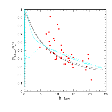
We investigate the dark matter excess in our simulated galaxies as follows. Figure 5 shows the contribution of the baryons to the total circular velocity for the sample galaxies of Piz05 with $V_{c}>$150 km/sec; these are plotted as a function of the “scaled” radius $\tilde{R}=R\left(\frac{220}{V_{c}}\right)$ (so as to scale all galaxies to approximately the same linear extent), where $R$ equals 2.2 scalelengths. The heavy lines show the mass ratio profile $(M_{*}/M_{tot})(<R)$, also scaled in terms of $\tilde{R}$, for two simulated Milky Way–type galaxies ($V_{c}\sim 230-250$ km/sec). The faint lines display, for one of these two galaxies, the $(V_{2.2,bar}/V_{c})^{2}$ profile we estimate by “redistributing” the disc mass according to its empirically expected scalelength, as discussed in Section 2.1 for the determination of the circular speed. The two faint lines correspond to two different assumptions for the B/D ratio (0.5 for the solid line, 0 for the dashed line).

Three cases, where the stellar mass inferred by Piz05 is actually larger than allowed by the rotational speed, i.e. $(V_{2.2,bar}/V_{c})^{2}>1$, have been excluded. We recall here that a “maximal disc” typically contributes to 85% of the rotation curve at 2.2 scalelengths (Sackett 1997), or $(V_{2.2,bar}/V_{c})^{2}\sim 0.7$. A few of the galaxies in the Piz05 sample seem thus to be “supermaximal”. Excluding such objects from the discussion, it seems that our simulations trace the cumulative baryonic mass fraction reasonably well, once we consider radii sufficiently far out.

As detailed in Section 2.1, we compute our $V_{2.2}$ adopting some “empirically corrected” scalelength and disc mass distribution, to avoid the known problem of too small and concentrated discs, which could bias our $V_{c}$ measurement in the simulations. This should limit the “cusp” influence on our $V_{c}$ estimate, and Fig. 5 shows that this is indeed the case for large enough radii. For a Milky Way–type galaxy ($V_{c}\sim$220 km/sec, $h_{I}\sim$3.5 kpc) we estimate $V_{c}$ at about 8 kpc, where indeed the baryon/DM proportion in the rotation curve looks realistic.

3.2.2 A bias to larger scalelengths?

Possibly contributing to the TF discrepancy in Fig. 3c is the fact that the SDSS spirals of the Piz05 sample have significantly larger scalelengths than the average relation holding for the larger and more representative Mathewson sample, which we have adopted for our scalelength correction (Fig. 2). That the Piz05 sample is biased to large scalelengths, possibly as a results of their extreme sample selection (B/D)${}_{i}\leq 0.1$, is also highlighted by Dutton et al. (2006). We have checked whether adopting the Piz05 $V_{c}$–scalelength relation to select (further out than before) the radius $R=2.2$ scalelengths where to measure our $V_{2.2}$, would reduce the offset in Fig. 3c; but the effect on the estimated $V_{c}$ is less than half the offset. So, larger scalelengths are not the full solution and the cause of the TF offsets must lie elsehwere.

3.2.3 A different Initial Mass Function?

One possible culprit is the adopted stellar IMF: the Kroupa IMF is a “bottom–light” IMF yet it is still at least 10% too “heavy” than required to reproduce the zero–point of the I band TF relation (see e.g. Fig. 4 in PST04); however a further 10% or 0.1 mag offset still would not reconcile simulations and observations in Fig. 3b. It is noteworthy though in this respect, that the Milky Way itself, whose chemical and photometric properties are well described by a Kroupa IMF, is also underluminous by about 1 $\sigma$ with respect to the observed TF relation (Flynn et al. 2006; see the data point with errorbars in Fig. 3), this is about the same offset as our simulations. Indeed the Milky Way lies much closer to the TF locus of the simulated galaxies, than to the empirical TF relation — namely, our simulations with the Kroupa IMF nicely match the Milky Way but not the TF normalization. This may suggest that the typical average IMF of external disc galaxies is more “bottom–light” than the local Solar Neighbourhood one (see also Gnedin et al. 2006).

The effect of changing the IMF (to a more bottom–heavy one) is shown by the two lower resolution runs simulated with the Salpeter IMF, represented by the S symbols in Fig. 3; in panels a and b, only the colour–corrected location of these two galaxies is shown for simplicity, to be compared to the open symbols for the Kroupa IMF galaxies. The $M_{*}/L$ ratio of the Salpeter IMF is higher, therefore the S galaxies define a significantly dimmer zero–point for the B and I-band TF relation. However, the stellar (or baryonic) mass TF normalization is hardly affected by the change in the IMF (and by the related change in supernova rates, feedback and chemical enrichment efficiency, gas restitution rate etc.): the baryonic mass that cools out to form the stellar disc correlates with the resulting circular velocity, so that data points in the ($M_{*},V_{c}$) plane tend to move along the TF locus leaving the zero–point unaffected (Navarro & Steinmetz 2000a,b).

Likewise, adopting a more bottom–light IMF than the Kroupa one in the simulations would also hardly affect the stellar mass TF locus. However, the $M_{*}/L$ ratio would be lower hence the TF locus would be brighter in the ($L,V_{c}$) plane. Besides, the observed stellar/baryonic mass TF relation in Fig. 3c,d would be lighter if a more bottom light IMF were assumed to translate multi–band photometry to stellar mass.

3.2.4 A different Universe?

A little bias in $M_{*}/L$ ratio is also expected from our choice of $h=0.65$, which makes our simulated Universe and galaxies $\sim$1 Gyr older than with the presently more popular choice of $h=0.7$. Systematically larger galaxy ages indeed correspond to systematically larger $M_{*}/L$ ratios, even for the same colour; but the effect over just 1 Gyr age offset is expected to be minor (Bell & de Jong 2001). One of the two Salpeter galaxies in Fig. 3 is actually run in a $h=0.7$, $\sigma_{8}=0.9$ Universe; but no significant difference in its TF location is seen, with respect to the other Salpeter galaxy; hence the effect of the younger Universe is minor.

The zero–points of simulated TF relations also depends on the cosmological parameters, especially $\Omega_{0}$ and $\sigma_{8}$, via the baryon fraction and the concentration of the dark matter haloes (Avila–Reese, Firmani & Hernández 1998; van den Bosch 2000; Navarro & Steinmetz 2000a,b; Eke, Navarro & Steinmetz 2001; Buchalter, Jimenez & Kamionkowski 2001). Our simulations are run in the “concordance” $\Lambda$CDM model — and as mentioned in the previous paragraph, choosing $\sigma_{8}=1.0$ over 0.9 does not make a significant difference; but the present “concordance” on the exact cosmological parameters is not perfect and values as low as $\Omega_{M}=0.26$ and especially $\sigma_{8}=0.74$ are advocated by the recent 3–year WMAP data release (Spergel et al. 2006; see also van den Bosch, Mo & Yang 2003). This revised cosmology results in lower halo concentrations, aiding the match with the zero–point of the TF relation (Gnedin et al. 2006), although some further effects counteracting adiabatic contraction may still need to be invoked (Dutton et al. 2006).

3.2.5 Adiabatic contraction?

We have also examined the role of adiabatic contraction with some additional experiment on our most massive simulated galaxy (at $V_{c}\sim 250$ km/sec). An excess in adiabatic contraction of the dark halo may occur in our simulations following the high baryonic concentration, as the angular momentum problem is not fully resolved, especially for massive galaxies. Although, when we compute $V_{c}$, we correct for the remaining angular momentum problem by “redistributing” the disc mass according to the empirically expected scalelength, we do not usually correct for the exceeding dark matter “pinching” that has occurred. The resulting dark matter content of our simulated galaxies within 2.2 scalelengths (the radius where we measure $V_{c}$) is of the order of 50%, ranging from 0.4–0.45 for our most massive objects ($V_{c}\sim$200–250 km-sec) to 0.55–0.6 for the dwarfs (100–120 km/sec).

For our most massive galaxy, we estimate the significance of the over–pinching by slowly (adiabatically) removing the present stellar disk+bulge, and inserting instead a pure exponential disk of mass $6.9\times 10^{10}$ $M_{\odot}$, and scalelength $R_{d}=3.8$ kpc (cf. SGP03). The resulting $V_{c}$ is reduced by less than 3%. Even neglecting adiabatic contraction completely, by combining the expected baryonic disc profile described above with the dark halo profile resulting from a DM–only simulation of the same object, reduces the resulting $V_{c}$ by only 6% or so. The effects of adiabatic contraction are by far not enough to cure the TF offsets in Fig. 3; in fact adiabatic expansion has been recently invoked in the literature to match the TF zero–point (Dutton et al. 2006).

Possibly a combination of all the contributing effects discussed above will help reproducing the zero–point of the TF relation; however, we remark that some uncertainty may still exist in the empirical zero–point itself: as mentioned above, the Milky Way for instance is also underluminous with respect to it (Flynn et al. 2006; see Fig. 3b). Also, for some of the existing normalizations, e.g. the Pierce & Tully (1992) TF relation which is still widely used as a local reference for TF evolution studies, no significant discrepancy remains once the colour correction is accounted for (Fig. 3a).

Figure 6: (a) B band and (b) stellar mass TF relation of simulated galaxies at $z=0$ (circles), $z=0.7$ (triangles) and $z=1$ (filled squares; open squares trace a few objects analyzed at $z=0.8$ instead of $z=1$). For a few objects, the evolution from $z=1$ to 0 is connected by a thin line for the sake of example. The size of the dots increases with the numerical resolution of the corresponding simulation. For $V_{c}<150$ km/s, only “long softening” (ls) simulations are shown for clarity. The solid, long–dashed and short–dashed lines are least square fits to the TF relation at $z=0$, $z=0.7$ and $z=1$ respectively.

4 The evolution of the Tully–Fisher relation

In this section we analyze the evolution of the TF relation as predicted by our simulations, both in terms of luminosity and of stellar mass.

In Fig. 6a we plot the TF relation in the B band for our simulated galaxies at different redshifts: $z=0$ (full circles), $z=0.7$ (triangles) and $z=1$ (full squares). Two of the simulated galaxies are quite disturbed at $z=1$ and were analyzed at $z=0.8$ instead (open squares). The solid, long dashed and short dashed lines are least square fits to the data points at $z=0$, 0.7 and 1 respectively. (The dotted symbols, representing the special “no late infall” experiment discussed in Section 5, are excluded from the fit). For circular velocities $V_{c}<150$ km/s, only ns mode simulations are shown in Fig. 6 and included in the various fits. This is just for the sake of clarity in the figure, as we verified that including the ls simulations does not change the overall picture nor the fits significantly. It is clear from Fig. 6a that the TF relation is predicted to evolve in luminosity, maintaining the slope nearly constant — notice in fact that that we did not impose a constant slope in the formal fits of Fig. 6a. The slope is around 8, i.e. close to $x=3$ when expressed as $L\propto V_{c}^{x}$, as expected in the current cosmological scenario (Navarro & Steinmetz 2000; Sommer-Larsen 2006). The evolutionary offset with respect to the $z=0$ relation is $\Delta M_{B}\sim 0.7$ mag at $z=0.7$ and $\Delta M_{B}\sim 0.85$ mag at $z=1$. This is somewhat intermediate in the range of current literature results (see the Table 1 in the introduction), but is certainly not compatible with very mild luminosity evolution.

The two galaxies analyzed at $z=0.8$ (because too disturbed at $z=1$; open squares in Fig. 6) appear to be slightly overluminous with respect to other “quiet” objects at $z=1$; this suggests that recent disturbance or dynamical interactions may enhance the luminosity with respect to the “normal” TF relation, as found in the local TF samples by Kannappan & Barton (2004). We verified, however, that their inclusion in the $z=1$ fit has negligible effects, hence they are considered together with all the other $z=1$ objects.

The luminosity evolution in Fig. 6a is driven by aging and dimming of the stellar populations hosted in the galaxies; while in terms of stellar mass, the evolution of the TF relation up to $z=1$ is rather negligible (Fig. 6b). At a given circular velocity, the increase in stellar mass between $z=1$ and $z=0$ is around 0.07–0.1 dex.

We stress, though, that the very mild evolution of the stellar mass applies only to the TF as a relation, but not to the individual objects, which typically grow by a factor of 1.5–2 in baryonic mass, between z=1 and z=0 (some examples of evolution of individual objects are connected by the thin lines in Fig. 6). As a consequence, interpreting the evolution of the TF relation as a pure luminosity evolution applied to the individual galaxy at fixed $V_{c}$ (e.g. Weiner et al. 2006) may be misleading. In fact, although the circular velocity of the inner dark halo regions is expected to evolve negligibly at late epochs (Mo et al. 1998; Wechsler et al. 2002), the growth of the disc mass by infall of halo gas and on–going star formation is necessarily accompanied by an increased disc contribution to the measured total $V_{c}$ of the galaxy, which thus grows in time. Because of the corresponding growth in stellar mass and circular velocity, however, the evolution of a given galaxy largely occurs along the TF relation so that the relation per se, considered at fixed $V_{c}$, evolves much less than the individual objects.

Recent observational results (Weiner et al. 2006) highlight indeed that the intercept of the TF relation evolves far more strongly in B band than in the near–infrared (J band), which is a closer tracer of stellar mass — although they also find a significant evolution in the slope, which we do not see in our simulated TF relation.

A dichotomy in the evolution of the TF relation observed in different bands was predicted also by e.g. Firmani & Avila–Reese (1999) and Buchalter et al. (2001). The latter results are qualitatively similar to ours, with a K band TF relation (closer to the actual stellar mass TF) that is very similar between $z=0$ and $z=1$, and a B band TF relation which is significantly brighter (and marginally steeper) at $z=1$. However the brightening they find is more significant than ours (larger than 1 mag); this is likely due to the fact that in their simplified models the disc is already in place at the redshift of formation, and after the initial peak (when the gas mass is largest) its star formation history is ever declining; hence their discs undergo purely passive evolution, while in our simulations they gradually build up via mergers, accretion and infall of halo gas — which must partly counteract the trend of passive luminosity dimming.

Firmani & Avila–Reese (1999), with their more detailed cosmological semi–numerical models, considered the TF relation in B band and in H band. They predict as well that the slope of the TF relation remains fixed with redshift, however they find that the H band TF zero–point gets significantly fainter at increasing redshift, in contrasts to our results of very minor evolution of the stellar mass TF relation. In the B band, the evolution of their TF zero–point reverses, but the brightening they find, out to $z\sim$1, is much milder than our results. The difference between our respective predictions apparently resides in the fact that in their model galaxies, while the stellar mass steadily increases, their $V_{max}$ remains roughly constant, rather than correlate with $M_{*}$ along the TF slope as we discussed above for our simulation.

The correlation we find between $V_{c}$ and $M_{*}$ may be artificially enhanced by an excess in adiabatic contraction of the dark halo following the high baryonic concentration of simulated galaxies. However, as we discussed in Section 3.2.5, the estimated effect of such “over–pinching” is less than 3%, therefore our $V_{c}$’s are likely not over–sensitive to the disc mass. Conversely, in the models of Firmani & Avila–Reese the baryonic disc possibly does not dominate enough the rotation curves and their $V_{max}$ does not correlate sufficiently with the disc mass; some correlation should indeed be expected since the baryonic contribution to rotation curves out to 2.2 scalelengths is prominent. In this sense, the evolution of the stellar mass TF relation can be considered as a probe of the baryon dominance and of the dark matter/baryon correlation in the rotation curve of disc galaxies.

5 A special “no late infall” experiment

For one of our simulations we run a special experiment, artificially halting infall of hot, dilute gas onto the disc at late times ($z<1$) by removing all low density gas (log($n_{H}$)$<-2$, log($T$)$>$30000 K) from the halo of the galaxy at $z=1$, leaving just two satellite galaxies in the halo.

This experiment is useful in view of the current debate on disc accretion: is a significant late infall of halo gas onto the disc compatible with the observed X–ray luminosity of galactic haloes (Toft et al. 2002; Rasmussen et al. 2004; Pedersen et al. 2005) and crucial for its build up, as typically assumed in standard galaxy formation scenarios? Or is disc galaxy evolution at late times driven by other mechanisms, like accretion of satellites (e.g. Helmi et al. 1999, 2006) or of cold gas (Birnboim & Dekel 2003; Binney 2005)? In this experiment, infall of hot and dilute halo gas is prevented, but satellite or cold gas accretion onto the galaxy can still occur.

Another useful application of this experiment is the evolution of disc galaxies in clusters: cluster spirals observed at intermediate redshifts apparently transform into passive spirals and S0’s by the present day (Dressler et al. 1997; Fasano et al. 2000; Smith et al. 2005), and quenching of star formation of the galaxies infalling onto the cluster is apparent from their photometric and spectroscopic properties (the Butcher–Oemler effect: Butcher & Oemler 1978, 1984, Ellingson et al. 2001, Margoniner et al. 2001, Kodama & Bower 2001; galaxies with k+a spectra: Dressler & Gunn 1983, Couch & Sharples 1987, Poggianti et al. 1999, 2004; or with emission lines: Lewis et al. 2002, Gomez et al. 2003). One of the possible culprits is the stripping of the halo gas reservoir when galaxies enter the cluster environment and the intra–cluster medium (ICM; Dressler 2004 and references therein). A crude way to simulate the ICM stripping is in fact to remove the hot, low density halo gas from the simulated galaxy.

In Fig. 3 this special experiment is indicated by the dotted circle at $V_{c}\sim 175$ km/s — and the corresponding “normal”, i.e. non–stripped, galaxy is marked by the triangle inscribed within a circle at $V_{c}\sim 185$ km/s. The effect of halo gas stripping is to reduce the fuel for star formation, thus reducing the final stellar mass and luminosity of the galaxy, as well as its circular velocity; the net effect is to let it settle on the same stellar-baryonic mass TF relation, albeit at a lower $V_{c}$ (Fig. 3cd). The stripped galaxy is fainter than the TF relation defined by the other galaxies (Fig. 3ab), but it is also significantly redder than its “normal” counterpart (Fig. 4) so that, once the colour correction is applied, the galaxy lies on the same TF relation as all the others (thin dotted circle in Fig. 3ab). Henceforth, with respect to TF properties the stripped galaxy at $z=0$ looks like a standard early–type spiral, fainter than the standard TF relation just due to its redder colours. As a “cluster spiral” experiment, this indicates that the TF relation for cluster galaxies at $z=0$ should not be markedly different from the field one of similar Hubble type, or once colour–corrections are applied. Notice though that we have only considered a relatively massive object for this experiment, while cluster environments may affect more importantly the TF relation at the low mass end (see Fig. 3c and the related discussion in Section 3).

In redshift, the stripped galaxy evolves more significantly in magnitude than the “normal” TF relation (Fig. 6a) and as an individual object its evolution occurs typically at constant $V_{c}$, as halo gas stripping has quenched its build–up by infall at $z>1$. This may hint to the possibility that, if halo gas infall were indeed irrelevant at late times, the TF relation would evolve more significantly than predicted by the standard simulations. Unfortunately, due to the present observational uncertainty in the TF evolution, it is not yet possible to distinguish between the various scenarios.

This experiment, artificially creating an early–type spiral, also highlights that the extent of the TF evolution likely depends on the final Hubble type of the spirals considered: the TF for early type galaxies is likely to evolve more significantly than that of late–type galaxies. When studying high redshift samples however, one hardly knows whether one is sampling the progenitors of Sa’s or of Sc’s, hence it may be misleading to compare to standard literature Sbc-Sc TF samples at $z=0$ born chiefly as distance indicators (e.g. Pierce & Tully 1992). The Hubble–type effect might contribute to the present wide range of results obtained by different authors on the TF relation. As pointed out by Kannappan & Barton (2004), one should rather compare to a volume–limited local sample selected with analogous criteria as the high–redshift one; not only to include in the comparison the role of dynamical disturbances that may bias the high–$z$ samples bright (and lead to overestimate the TF evolution), but also to compare locally to a fair mixture of Hubble types: if the local TF relation is preferentially based on the (brighter) Sbc-Sc types, the corresponding TF evolution may be underestimated. The Hubble type effect is by no means negligible: from Sc to Sb to Sa, TF offsets of 0.4 to 0.7 mag are found (Kannappan et al. 2002; PST04), i.e. significant with respect to the observed amount of TF evolution (0–1.5 mag, see the Introduction).

Clearly the evolution of the stellar mass TF relation bypasses the Hubble type bias, however this is much more demanding observationally as multi–band data are required.

6 Summary and conclusions

In this paper we discuss the TF relation and its evolution as predicted by cosmological simulations of disc galaxy formation including hydrodynamics (Tree-SPH) and all the relevant baryonic physics, such as star formation, chemical and photometric evolution, metal–dependent cooling, energy feedback.

The resulting disc galaxies at $z=0$ have scalelengths compatible with the observed ones in the low–mass range ($V_{c}\sim$100–120 km/sec), and somewhat shorter, yet within a factor of 2, for Milky Way–type or more massive objects. Though still somewhat plagued by the angular momentum problem, our physical recipe and implementation of strong early feedback goes a long way in creating realistic galaxies (SGP03).

At $z=0$, the TF relation defined by our simulated galaxies is offset by about 0.4 mag in luminosity, and by about 40% in stellar (and baryonic) mass, with respect to observational TF relations. This is a well known problem of galaxy formation simulations (Navarro & Steinmetz 2000) and the origin of the offset remains somewhat unclear. We demonstrate that it is likely not due to the dark matter cusp in the central regions, and that it cannot be cured by simply avoiding adiabatic contraction. A different choice of cosmological parameters (such as $\sigma_{8}$) and/or of stellar IMF in disc galaxies may concur to solve the problem; some mechanism for adiabatic expansion of the halo from the baryons has also been recently invoked in this respect (Dutton et al. 2006).

However, we remark that the location of the Milky Way with respect to the TF relation is also offset (Flynn et al. 2006), by as much as our simulations. The fact that our Galaxy lies on the same TF locus as our simulations adopting a Solar Neighbourhood–like IMF (Fig. 3), suggests the puzzling possibility that the problem may not lie with the simulations or the cosmology, but rather with the luminosity zero–point of the observed TF relation of external galaxies, or with the IMF of the Milky Way which may not be representative for all disc galaxies.

As to the luminosity evolution of the TF relation with redshift, there is presently no consensus observationally, with estimates ranging from negligible evolution to $\Delta M_{B}>$1 mag by $z\sim$1. Also, there are claims that the evolution may be mostly in the slope (with a stronger brightening for lower mass objects) rather than a systematic offset, but this also is still debated. There is however some preliminary consensus that the stellar mass TF relation hardly evolves out to $z\sim$1.

Our simulations predict a significant B–band luminosity evolution ($\Delta M_{B}$=0.7 mag by $z$=0.7 and $\Delta M_{B}$=0.85 mag by $z$=1), while the TF slope remains nearly constant (systematic zero–point evolution). The redshift evolution of the TF relation is a result of the correlated increase in stellar mass and $V_{c}$ in the individual galaxies, combined with luminosity fading and reddening caused by the aging of the host stellar populations. At fixed $V_{c}$, the net effect is a systematic decrease in B band luminosity, while in terms of stellar mass the TF relation hardly evolves at all, in agreement with the present available observational evidence.

This does not mean that the stellar mass content of the individual galaxies does not evolve: each galaxy grows typically by 50–100% in mass between $z=1$ and $z=0$, but as its baryonic mass grows, its circular velocity also increases so that the evolution of the individual object occurs largely along the TF relation. The relation as such does not show any significant evolution.

We also consider as a special experiment a simulation where late gas infall on the disc is precluded, by artificially stripping the galaxy of its hot, dilute halo gas at $z=1$. This is useful to assess alternative scenarios of disc galaxy formation, where late disc growth is driven by other processes (like satellite or cold gas accretion), as well as a possible scenario of spiral evolution in clusters, where ram pressure stripping from interaction with the ICM is a possible driver of morphological transformations. We find that, from the point of view of the TF properties, the resulting object is indistinguishable from early type spirals with little recent star formation and red colours — henceforth the TF relation for cluster galaxies at $z=0$ should not be markedly different from the field one, once colour–corrections are applied. Its TF evolution is however more significant than that of the “normal” simulations, suggesting that, if halo gas infall had no major role in disc galaxy evolution at late times, the TF relation would show a much stronger luminosity evolution. Unfortunately the present observational uncertainty does not allow to discuss if either scenario is really favoured. This experiment, artificially creating an early–type galaxy, also underlines that the amount of TF evolution likely depends on Hubble spiral type, being more significant for early types; this effect might contribute to the discrepancy between different observational results, and should be taken into account when selecting the local reference TF sample.

References

- [1] Abadi M.G., Navarro J.F., Steinmetz M., Eke V.R., 2003, ApJ 597, 21
- [2] Avila–Reese V., Firmani C., Hernández X., 1998, ApJ 505, 37
- [3] Bamford S.P., Milvang-Jensen B., Aragon-Salamanca A., 2006, MNRAS 366, 308
- [4] Barden M., Lehnert M.D., Tacconi L., Genzel R., White S., Franceschini A., 2003, submitted to ApJ Letter (astro-ph/0302392)
- [5] Bell E.F., de Jong R.S., 2001, ApJ 550, 212
- [6] Bell E.F., McIntosh D.H., Katz N., Weinberg M.D., 2003, ApJS 149, 289
- [7] Binney J., 2005, in Extra–Planar Gas, R. Braun (ed.), ASP Conf. Series vol. 331, p. 131
- [8] Böhm A., Ziegler B.L., 2006, submitted to ApJL (astro-ph/0601505)
- [9] Böhm A., et al. 2004, A&A 420, 97
- [10] Boissier S., Prantzos N., 1999, MNRAS 307, 857
- [11] van den Bosch F.C., 2000, ApJ 530, 177
- [12] van den Bosch F.C., Mo H.J., Yang X., 2003, MNRAS 345, 923
- [13] Buchalter A., Jimenez R., Kamionkowski M., 2001, MNRAS 322, 43
- [] Butcher H., Oemler A., 1978, ApJ 226, 559
- [] Butcher H., Oemler A., 1984, ApJ 285, 426
- [14] Conselice C.J., Bundy K.E., Richard S., Brichmann J., Vogt N.P., Phillips A.C., 2005, ApJ 628, 160
- [] Couch W.J., Sharples R.M., 1987, MNRAS 229, 423
- [15] Dalcanton J.J., Spergel D.N., Summers F.J., 1997, ApJ 482, 659
- [] Dressler A., 2004, in Clusters of galaxies: probes of cosmological structure and galaxy evolution, J.S. Mulchaey , A. Dressler and A. Oemler (eds.), Carnegie Observatories Astrophysics Series, vol. 3 (Cambridge: Cambridge Univ. Press), p. 207
- [] Dressler A., Gunn J.E., 1983, ApJ 270, 7
- [] Dressler A., Oemler A., Couch W.J., Smail I., Ellis R.S., Barger A., Butcher H., Poggianti B.M., Sharples R.M., 1997, ApJ 490, 577
- [16] Dutton A., van den Bosch F.C., Dekel A., Courteau S., 2006, submitted to ApJ (astro-ph/0604553)
- [17] Eke V., Navarro J.F., Steinmetz M., 2001, ApJ 554, 114
- [] Ellingson E., Lin H., Yee H.K.C., Carlberg R.G., 2001, ApJ 547, 609
- [] Fasano G., Poggianti B.M., Couch W.J., Bettoni D., Kjærgaard P., Moles M., 2000, ApJ 542, 673
- [] Firmani C., Avila–Reese V., 1999, in Observational Cosmology: the Development of Galaxy Systems, G. Giuricin, M. Mezzetti and P. Salucci (eds.), ASP Conf. Series vol. 176, p. 406
- [] Flynn C., Holmberg J., Portinari L., Fuchs B., Jahreiß H., 2006, MNRAS 372, 1149
- [] Flores H., Hammer F., Puech M., Amram P., Balkowski C., 2006, A&A 455, 107
- [] Gnedin O.Y., Weinberg D.H., Pizagno J., Prada F., Rix H.-W., 2006, submitted to ApJ (astro-ph/0607394)
- [] Gomez P.L., et al., 2003, ApJ 584, 210
- [18] Governato F., Willman B., Mayer L., Brooks A., Stinson G., Valenzuela O., Wadsley J., Quinn T., 2006, MNRAS in press (astro-ph/0602351)
- [19] Haardt F., Madau P., 1996, ApJ 461, 20
- [20] Helmi A., White S.D.M., de Zeeuw P.T., Zhao H., 1999, Nature 402, 53
- [21] Helmi A., Navarro J., Nordström B., Holmberg J., Abadi M., Steinmetz M., 2006, MNRAS 365, 1309
- [22] Kannappan S.J., Barton E.J., 2004, AJ 127, 2694
- [23] Kannappan S.J., Fabricant D.G., Franx M., 2002, AJ 123, 2358
- [24] Kodama T., Bower R.G, 2001, MNRAS 321, 18
- [] Lewis G.F., Babul A., Katz N., Quinn T., Hernquist L., Weinberg D.H., 2000, ApJ 526, 623
- [] Margoniner V.E., de Carvalho R.R., Gal R.R., Djorgovski S.G., 2001, ApJ 548, L143
- [25] McGaugh S.S., 2005, ApJ 632, 859
- [26] Milvang–Jensen B., Aragón–Salamanca A., Hau G.K.T., Jørgensen I., Hjorth J., 2003, MNRAS 339, L1
- [27] Mo H.J., Mao S., White S.D.M., 1998, MNRAS 295, 319
- [28] Navarro J.F., Steinmetz M., 2000a, ApJ 528, 607
- [29] Navarro J.F., Steinmetz M., 2000b, ApJ 538, 477
- [30] Pedersen K., Rasmussen J., Sommer–Larsen J., Toft S., Benson A.J., Bower R.G, 2005, NewA 11, 465
- [31] Pierce M.J., Tully R.B., 1992, ApJ 387, 47
- [32] Pizagno J., et al. 2005, ApJ 633, 844 (Piz05)
- [] Poggianti B.M., Smail I., Dressler A., Couch W.J., Barger A.J., Butcher H., Ellis R.S., Oemler A., 1999, ApJ 518, 576
- [] Poggianti B.M., Bridges T.J., Komiyama Y., Yagi M., Carted D., Mobasher B., Okamura S., Kashilawa N., 2004, ApJ 601, 197
- [33] Portinari L., Sommer–Larsen J., Tantalo R., 2004, MNRAS 347, 691 (PST04)
- [34] Press W.H., Teukolsky S.A., Vetterling W.T., Flannery B.P., 1992, Numerical Recipes, Cambridge University Press
- [35] Rasmussen J., Sommer–Larsen J., Toft S., Pedersen K., 2004, MNRAS 349, 255
- [36] Rigopoulou D., Franceschini A., Aussel H., Genzel R., Thatte N., Cesarsky C.J., 2002, ApJ 580, 789
- [37] Rix H.-W., Guhathakurta P., Colless M., Ing K., 1997, MNRAS 285, 779
- [38] Roberts M.S., Haynes M.P., 1994, ARA&A 32, 115
- [39] Romeo A.D., Portinari L., Sommer–Larsen J., 2005, MNRAS 361, 983
- [40] Romeo A.D., Sommer–Larsen J., Portinari L., Antonuccio–Delogu V., 2006, MNRAS 371, 548
- [41] Sackett P.D., 1997, ApJ 483, 103
- [42] Simard L., Pritchet C.J., 1998, ApJ 505, 96
- [] Smith G.P., Treu T., Ellis R.S., Moran S.M., Dressler A., 2005, ApJ 620, 78
- [43] Smith J.K., et al. 2004, MNRAS 354, L19
- [44] Sommer–Larsen J., Dolgov A., 2001, ApJ 551, 608
- [45] Sommer–Larsen J., Götz M., Portinari L., 2003, ApJ 596, 47 (SGP03)
- [46] Sommer–Larsen J., 2006, ApJ 644, L1
- [47] Spergel D.N., et al. 2006, submitted to ApJ (astro-ph/0603449)
- [48] van Starkenburg L., van der Werf P.P., Yan L., Moorwood A.F.M., 2006, A&A 450, 25
- [49] Toft S., Rasmussen J., Sommer–Larsen J., Pedersen K., 2002, MNRAS 335, 799
- [50] Tully R., Fouqué P., 1985, ApJS 58, 67
- [51] de Vaucouleurs G., de Vaucouleurs A., Corwin H.G., Buta R.J., Paturel G., Fouqué P., 1991, Third Reference Catalogue of Bright Galaxies, Springer–Verlag
- [52] Vogt N.P., 1999, in The Hy Redshift Universe, A.J. Bunker and W.J.M. van Breugel (eds.), ASP Conf. Series vol. 193, p. 145
- [53] Vogt N.P., 2006, in Island Universers — Structure and Evolution of Disk Galaxies, R.S. de Jong (ed.), Springer, in press
- [54] Vogt N.P., Forbes D.A., Phillips A.C., Gronwall C., Faber S.M., Illingworth G.D., Koo D.C., 1996, ApJ 465, L15
- [55] Vogt N.P., et al. 1997 ApJ 479, 121
- [56] Wechsler R.H., Bullock J.S., Primack J.R., Kravtsov A.V., Dekel A., 2002, ApJ 568, 52
- [57] Weiner B.J., et al. 2006, ApJ in press (astro-ph/0609091)