New ”Bigs” in cosmology

Abstract

This paper contains a detailed discussion on new cosmic solutions describing the early and late evolution of a universe that is filled with a kind of dark energy that may or may not satisfy the energy conditions. The main distinctive property of the resulting space-times is that they make to appear twice the single singular events predicted by the corresponding quintessential (phantom) models in a manner which can be made symmetric with respect to the origin of cosmic time. Thus, big bang and big rip singularity are shown to take place twice, one on the positive branch of time and the other on the negative one. We have also considered dark energy and phantom energy accretion onto black holes and wormholes in the context of these new cosmic solutions. It is seen that the space-times of these holes would then undergo swelling processes leading to big trip and big hole events taking place on distinct epochs along the evolution of the universe. In this way, the possibility is considered that the past and future be connected in a non-paradoxical manner in the universes described by means of the new symmetric solutions.

I Introduction

Current research in cosmology is a very exciting, rapidly evolving endeavor. It is actually one which however typically attracts the kind of rejections that some scientists use to make against every new idea or development in cosmology and that have successively dismissed big bang, black holes, inflation, cosmic strings, wormholes and, ultimately, accelerating expansion and phantom energy. However, observational data are rather obstinate in favour of the two latter suggestions and thereby of the previous one Hannestad . In fact, sometimes the point is not so much if a particular theory or interpretation is too much unusual or crazy, but, as it is believed Pauli told Heisenberg once, whether it is unusual or crazy enough. It is in this spirit that we have considered the subject of this paper which will deal with the three new ”bigs” that have recently arisen in the new standard cosmological scenario: the big rip Caldwell , the big trip Gonz1 and the big hole. Together with the big bang and big crunch, these new ”bigs” make up the most dramatic events that may have occurred or may eventually take place in the universe.

It appears already certain that the current universe is undergoing a period of accelerating expansion Perlm . What is still under discussion indeed is whether such an acceleration is or not beyond the barrier implied by a cosmological constant; that is whether the parameter $w$ of the equation of state $p=w\rho$ is or not exactly equal to -1. Actually, the case which each time appears to be most favoured by observations is that for a value of $w$ quite close to, but still less than -1 Hannestad . Nevertheless, no matter how close to -1 it could be, if $w<-1$ then our universe would be filled with some kind of phantom energy and its expansion would be super-accelerated. Phantom energy is a rather weird stuff indeed phantom . Besides its nice properties - which would include super-accelerated expansion and the possibility to describe primordial inflation Gonz2 - it is known to possess the following unusual characteristics. If dark energy is described by a scalar field $\phi$ with the FRW customary definitions, $\rho=\dot{\phi}^{2}/2+V(\phi)$, $p=\dot{\phi}^{2}/2+V(\phi)$, with $\rho$ and $p$ the energy density and pressure, respectively, and $V(\phi)$ the field potential, then (i) the kinetic term $\dot{\phi}^{2}/2<0$ and therefore phantom cosmologies suffer from violent instabilities and classical inconsistencies, (ii) the energy density is an increasing function of time which would make the quantum-gravity regime to appear also at late times, (iii) the dominant energy condition is violated so that $\rho+p<0$, and (iv) there will be a singularity in the finite future dubbed big rip at which the universe ceases to exist and near of which there may appear cosmic violations of causality. These properties define phantom energy in the quintessence scenario.

The present paper aims at considering big rips and big trips, so as the newest possible phenomenon that might also occur in the future and that we shall here denote by big hole, in the context of new cosmological solutions where such events will all take place not just in the future but also in the past and the definitions of dark and phantom energy are generalized. We shall first review in a few more detail what is understood by big rip, big trip and big hole in usual quintessence when the equation of state is $p=w\rho$. Using the general expression

$$\frac{\dot{\rho}}{\rho}=-3H(1+w)=\frac{2\dot{H}}{H},$$ (1)

where $H=\dot{a}/a$ and $w$ is taken to be constant, we can derive expressions for the scale factor $a(t)$ and the energy density in the quintessence model to be

$$a(t)=\left[a_{0}^{3(1+w)/2}+\frac{3}{2}C(1+w)(t-t_{0})\right]^{2/[3(1+w)]},$$ (2)

in which $C$ is a constant and the universe speed-up anyway, and

$$\rho(t)=H^{2}=\frac{C^{2}}{\left[a_{0}^{3(1+w)/2}+\frac{3}{2}C(1+w)(t-t_{0})\right]^{2}}...$$ (3)

Now, in the phantom regime defined by $w<-1$, it can be seen that $\rho$ increases with $t$ up to the time

$$t=t_{*}=t_{0}+\frac{2a_{0}^{-3(|w|-1)/2}}{3C(|w|-1)},$$ (4)

at which it diverges. It can be seen that the scale factor $a(t)$ also blows up at $t=t_{*}$. This curvature singularity is what we call big rip Caldwell . If no pathological space-time branches would connect the super-accelerating expanding region before the big rip to the contracting region after it transmitting physical information, then the big rip would mark the end of the universe and everything in it. In the quintessence model phantom energy will therefore be characterized by $\rho>0$, $\rho+p<0$, $\dot{\phi}^{2}<0$, a big rip singularity at $t=t_{*}$ and a positive definite potential

$$V(\phi)=\frac{1}{2}(|w|+1)C^{2}e^{-3i\sqrt{|w|-1}(\phi-\phi_{0})},$$ (5)

with

$$\phi(t)=\phi_{0}-\frac{2i}{3\sqrt{|w|-1}}\log\left[\left(\frac{a_{0}}{a}\right)^{3(|w|-1)/2}\right],$$ (6)

in which $\phi_{0}$ is another constant.

On the other hand, it has been shown that phantom energy makes the kind of stuff that leads to formation of Lorentzian Morris-Thorne wormholes Lobo . Therefore such wormholes would be expected to copiously crop up in a universe dominated by phantom energy. Now, once they are formed with a size small enough as to be stable against vacuum polarization, these wormholes would start accreating phantom energy to induce a swelling process in the wormhole spacetime that inflates their throat so quickly that, relative to an asymptotic observer, they would engulf the universe itself at a time in the future given by Gonz1

$$\tilde{t}=t_{0}+\frac{1}{\beta+\frac{3}{2}Ab_{0}(|w|-1)},$$ (7)

where $b_{0}$ is the initial radius of the spherical wormhole throat, $\beta$ is a constant and $A$ is a numerical coefficient of order unity. Thus, the universe would find itself passing through the tunneling from one mouth to the other at a time that precedes the big rip for a presumably short while and that, depending on the relative kinematic characteristics of the resulting insertions of the two wormhole mouths, might make the universe travel in time toward the past or future. This traveling is what has been dubbed big trip Gonz1 and, far from being a catastrophic event, it really could offer a possibility of escaping from the doomsday implied by the big rip.

Finally, let us consider what we mean here by a big hole. It is now a matter of common wisdom that our universe contains many black holes whose sizes ranges from a few solar masses to several billions of solar masses. The latter black holes are called supermassive and are thought to be placed at the galactic centres. Any of such black holes would accrete dark energy with $w>-1$ in a process that parallels phantom energy accretion by wormholes and that would in principle lead to a swelling of their event horizon so gigantic that eventually the black hole would finally swallow the whole universe in the finite future, at a time Prado

$$t_{bh}=t_{0}+\frac{1}{[\frac{3}{2}B\rho_{0}M_{0}-(6\pi\rho_{0})^{1/2}](1+w)},$$ (8)

where $M_{0}$ is the initial mass of the black hole, $\rho_{0}$ is the initial energy density and $B$ is a numerical constant of order unity. When dealing with quintessence models, this black hole swelling becomes an irrelevant process however. In fact, putting reasonable astronomical data in Eq. (1.8) allows us to discover that in this case the accretion of dark energy could only significantly modify the black hole size if the initial black hole mass would be of the order of the total mass of the universe, a situation which can never be expected to occur along the entire evolution of the universe Prado . It will be seen nevertheless that in the context of the cosmological models that will be considered in this paper black holes can perfectly undergo a big hole process.

The paper is organized as follows. In Section II we shall deal with two new phantom cosmological solutions to represent the space-time of an accelerating universe. What is new about such solutions is that, in addition to showing a big rip in the future, they also predict a big rip in the past, and that the nature of its phantom energy is dual to that for phantom energy in usual quintessential solution. Sec. III contains a study of the accretion of phantom energy by wormholes and black holes in the space-times described by the new solutions. It will be shown that in such universes there will be multiple big trips and big holes, depending on the cosmic time on which the observer is placed. The possibility that the future and past be connected by means of black hole and wormhole swellings in this kind of cosmologies is discussed in Sec. IV. Finally, we conclude and add some comments in Sec. V. Throughout the paper we use units such that $8\pi G/3=c=1$.

II Cosmic solutions with two big rips

In this section we shall consider two new cosmological solutions that correspond to super-accelerated versions beyond the De Sitter space as given in the form $a=H_{0}^{-1}\cosh(H_{0}t)$, i.e. to space-times that evolves both in positive and negative time and can be shown to be symmetric relative to $t=0$.

Let us consider first a solution described by a scale factor of the form

$$a(t)=\alpha\left(\beta+x\tan x\right),$$ (9)

where $x=\kappa t$, $\kappa$, $\alpha$ and $\beta$ are all positive constants. We will study this solution in the interval $-t_{R}<t<t_{R}$, where $t_{R}=\pi/2\kappa$. We shall hereafter refer to the scale factor (2.1) as solution I. In Fig 1 we give a plot of such a solution which can be obtained by using the Darboux transormation x1 .

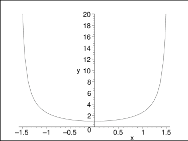
Figure 1: Evolution of solution I with time from a big rip in the past to a big rip in the future.

It is easy to see that $a(\pm t_{R})=+\infty$, i.e. there is big rip singularities at $t=\pm t_{R}$. Moreover, on the subinterval $-t_{R}<t<0$ the universe would go through a contracting stage which ends up at $t=0$, from which it starts expanding to finally end again up in a big rip at $t=+t_{R}$. Such a behavior is highly unusual indeed. Notice as well that $a(t)$ does not vanish at any points along the considered interval; the minimum value of the scale factor occurs at $a(0)=\alpha\beta$. Now, we show that the number of free parameters entering the scale factor (2.1) is efficiently sufficient to describe our observed universe; that is they can satisfy the following three conditions: they should reproduce (1) the current value of the Hubble constant, $H(t_{0})=H_{0}=h\times 0.324\times 10^{-19}$ s^-1, where $45<h<75$, (2) $\ddot{a}_{0}/a_{0}=7H_{0}^{2}/10$, and (3) $a_{0}\sim 10^{28}$ cm. We shall check in what follows that this is actually the case. In fact, replacing the solution (2.1) into the Friedmann equations for a flat universe, we get for the energy density

$$\rho=\frac{\kappa^{2}(T+x+xT^{2})^{2}}{(\beta+xT)^{2}}$$ (10)

and for pressure

$$p=-\frac{5\kappa^{2}x^{2}T^{4}+2x(2\beta+3)T(T^{2}+1)+(4\beta+6x^{2}+1)T^{2}+4\beta+x^{2}}{3(\beta+xT)^{2}},$$ (11)

where $T=\tan x$. We can then obtain an expression for the Hubble constant

$$H=\frac{\kappa(2x+\sin(2x))}{2\cos x(\beta\cos x+x\sin x)}$$ (12)

and

$$\rho+3p=-\frac{4\kappa^{2}(1+xT)}{(\beta+xT)\cos^{2}x}.$$ (13)

Since the combination given by Eq. (2.5) is definite negative we deduce that the strong energy condition is permanently violated and therefore the universe undergoes constant acceleration.

Let us now consider condition (2). We can write for the constant $\beta$

$$\beta=\frac{(80\cos^{2}x_{0}-52)x_{0}^{2}-12x_{0}\sin(2x_{0})+7\sin^{2}(2x_{0})}{80\cos x_{0}(x_{0}\sin x_{0}+\cos x_{0})}.$$ (14)

It can be seen that at small values of $x_{0}$ $,\beta$ behaves like an inverted Higgs potential (Fig. 2). The values which are of interest here are those that lead to positive $\beta$. Such values lie in the range $x_{0}<x_{m}\sim 0.6$. We can then evaluate the constant $\kappa$ to be

$$\kappa=\frac{7H_{0}\cos x_{0}(2x_{0}+\sin(2x_{0}))}{40(x_{0}\sin x_{0}+\cos x_{0})},$$ (15)

which in turn implies that

$$t_{0}=\frac{x_{0}}{\kappa}=\frac{40x_{0}(x_{0}\sin x_{0}+\cos x_{0})}{7H_{0}\cos x_{0}(2x_{0}+\sin(2x_{0}))}$$ (16)

and $t_{R}=\pi/(2\kappa)$. We can now calculate the length of time

$$\Delta t_{R}=t_{R}-t_{0}=\frac{(\pi-2x_{0})t_{0}}{2x_{0}}.$$ (17)

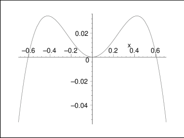
Figure 2: Evolution of parameter $\beta$ with time. At small $x_{0}$ it adopts the shape of an inverted Higgs potential.

The results of the numerical computations are summarized in the table. In the first row we give the different values of $x_{0}$ from $0.1$ up to $0.6$; in the second row- the least values of the scale factor, reached at $t=0$ during the change of regimes of expanding. Next two rows present the value $t_{0}$ for two limiting values of the Hubble constant: $h=45$ and $h=75$, correspondingly. This value is related to the time elapsed since the beginning of the universe expansion up to the present. The values of $\Delta t_{{}_{R}}$ for $h=45$ and $h=75$ are presented in the fifth and six rows. The last two rows contain the values computed for the age of the universe with respect to $h=45$ and $h=75$, respectively, i.e. the time passed from $t=-t_{{}_{R}}$ to $t=t_{0}$. All times in the Table are expressed in ordinary years.

$x_{0}$	0.1	0.2	0.3	0.4	0.5	0.6
$a_{min}$	$0.27a_{0}$	$0.26a_{0}$	$0.22a_{0}$	$0.17a_{0}$	$0.1a_{0}$	$0.01a_{0}$
$t_{0}/10^{9}$ (yr), h=45	$31.4$	$32.7$	$35$	$38.3$	$43$	$49.3$
$t_{0}/10^{9}$ (yr), h=75	$18.9$	$19.7$	$20.1$	$23$	$25.8$	$29.6$
$\Delta t_{{}_{R}}/10^{9}$ (yr), h=45	$463$	$225$	$148$	$112$	$92$	$80$
$\Delta t_{{}_{R}}/10^{9}$ (yr), h=75	$278$	$135$	$89$	$67$	$55$	$48$
$T/10^{9}$ (yr), h=45	$526$	$244$	$218$	$189$	$178$	$178$
$T/10^{9}$ (yr), h=75	$316$	$170$	$130$	$113$	$107$	$107$

A quite clearer physical motivation can be ascribed to a solution (which will be denoted as solution II) stemming from the Randall-Sundrum brane world model I RS where the Fiedmann equations can be written as

$$\frac{{\dot{a}}^{2}}{a^{2}}=\rho\left(1+\frac{\rho}{2\lambda}\right),$$ (18)

$$-2\frac{\ddot{a}}{a}=\rho+3p+\frac{\rho}{\lambda}\left(2\rho+3p\right).$$ (19)

The solution of the equations (2.10), (2.11) has the form

$$a^{6\epsilon}=\frac{s}{1-18\lambda\epsilon^{2}\left(t-t_{1}\right)^{2}},$$ (20)

where

$$\frac{p}{\rho}=w=-1-2\epsilon,$$

$\epsilon>0$, $t_{1}=$const and $s=$const.

Thus, to obtain the big rip singularities one need to choose $\lambda>0$. On the other hand, $a(t)$ must be positive so that $s>0$. We have two big rips at

$$t_{\pm}=t_{1}\pm\frac{1}{3\epsilon\sqrt{2\lambda}}.$$ (21)

A fully symmetric solution with the big rips symmetrically displayed around $t=0$ can immediately be obtained by choosing $t_{1}=0$

The energy density and pressure will be:

$$\rho=-\frac{2\lambda}{1-18\lambda\epsilon^{2}\left(t-t_{1}\right)^{2}}<0,$$ (22)

$$p=\frac{2\lambda(1+2\epsilon)}{1-18\lambda\epsilon^{2}\left(t-t_{1}\right)^{2}}>0.$$ (23)

Now, let consider the universe filled with scalar field $\phi$, such that

$$\rho=K+V,\qquad p=K-V,$$

with $K={\dot{\phi}}^{2}/2$, $V=V(\phi)$. Using (22) and (23) one gets

$$K=\frac{2\lambda\epsilon}{1-18\lambda\epsilon^{2}\left(t-t_{1}\right)^{2}}>0,$$ (24)

and

$$V=-\frac{2\lambda(\epsilon+1)}{1-18\lambda\epsilon^{2}\left(t-t_{1}\right)^{2}}<0.$$ (25)

Thus, in the brane world we have the highly nontrivial situation that a model with negative potential (and positive $K$) results in a big rip singularity.

One can see that

$$p+\rho=\frac{4\lambda\epsilon}{1-18\lambda\epsilon^{2}\left(t-t_{1}\right)^{2}}>0,$$

and

$$3p+\rho=\frac{4\lambda(1+3\epsilon)}{1-18\lambda\epsilon^{2}\left(t-t_{1}\right)^{2}}>0.$$

But since $\rho<0$ both weak and strong energy conditions are violated. It is interesting to note that

$$\frac{\ddot{a}}{a}=\frac{6\epsilon\lambda\left(6\lambda\epsilon(t-t_{1})^{2}+18\lambda\epsilon^{2}(t-t_{1})^{2}+1\right)}{1-18\lambda\epsilon^{2}\left(t-t_{1}\right)^{2}}>0.$$

We restore finally $V$ as a function $V(\phi)$. To do this one need to find $\phi=\phi(t)$ from Eq. (2.16), expressing then $t=t(\phi)$ to finally substitute it into Eq. (2.17). After simple calculation one get

$$\phi(t)=\phi_{0}\pm\frac{1}{3}\sqrt{\frac{2}{\epsilon}}{\rm arcsin}\left(3\epsilon\sqrt{2\lambda}(t-t_{1})\right),$$

and hence

$$V(\phi)=-\frac{2\lambda(\epsilon+1)}{{\rm cos}^{2}\left(3\sqrt{\frac{\epsilon}{2}}(\phi-\phi_{0})\right)},$$ (26)

where $\phi_{0}=$const. Note that in this case the field $\phi$ is real in spite of corresponding to a phantom stuff.

Thus, we have a model with positive tension, positive $K$, negative potential $V$, negative $\rho=K+V$ and positive pressure $p=K-V$. At the same time, $\rho+p>0$ ($\rho+3p>0$ too) and ${\ddot{a}}/a>0$. This universe is filled with a scalar field with the rather amusing potential (26).

We have two big rips at $t=t_{\pm}$ (see Eq. (21)). In the ”classical” limit $\lambda\to\infty$ we have only one big rip at $t=t_{1}$. Therefore, the situation with two big rips (initial and final) should be taken to be a brane effect.

It has been seen that inserting a parameter $w<-1$ in this brane world model leads to a distinct phantom stuff, one which is dual to the phantom energy resulting in quintessence with $w<-1$ in that in the present case it is the energy density $\rho$ but not $\rho+p$ what is negative definite. Moreover, dual phantom is associated with a scalar field with negative potential and positive kinetic term. The only prediction which is shared by phantom and dual phantom is the emergence of future (or past) singularities.

Actually usual phantom energy with negative scalar-field kinetic term appears to occur only in the regions before the first big rip at $t_{-}$ and after the second big rip at $t_{+}$ (see Fig. 3). Had we taken $w>-1$ in the precedent calculation then the resulting scale factor had described a universe initially contracting down to a singularity (a big crunch respect to an interior observer or a big bang respect to the exterior, following region) at $a=0$, both for positive and negative time, followed in the two branches by usual accelerating regions which extend toward infinity. It is worth noticing that in this case, whereas the exterior accelerating regions are filled with conventional dark energy, in the region between the two zeros dark energy would be also unusual in that it would be the dual (with negative values for $\rho$ and $\rho+p$) to conventional dark energy (Fig. 3). All the regions with dual stuffs would disappear in the limit $\lambda\rightarrow\infty$ where no brane is present. Therefore the existence of such regions and hence of a second big rip can be considered to be a pure brane effect.

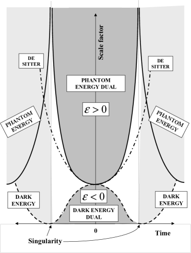
Figure 3: The different dark-energy and phantom-energy regions which can be obtained for Solution II. Dual regions correspond to the interval between the two symmetric (big bang or big rip) singularities and are originated from pure brane effects.

We note finally that at first sight it could seem unnatural to talk about big rip singularities and accelerating universe in a model of brane world which would be expected to describe the early universe. However, since the absolute value of the energy density is an increasing function of squared time in the present model, the brane and quantum effects are here expected to become relevant at late time, instead of at the early stages.

The brane symmetric solution, on the other hand, has a rather surprising property which can help to create and maintain a shortcut for interstellar travel. In fact, following Krasnikov Kras1 one can define a shortcut as follows. Let $C$ be the timelike cylinder in Minkowski space $L^{4}$, $M$ a globally hyperbolic spacetime and $U$ a subset of $M$. Then $U$ will be a shortcut if the isometry $\kappa:(M-U)\to(L^{4}-C)$ and two points $p$ and $q$ exist such that $p\preceq q$ (i.e. there is a future-directed timelike curve from $p$ to $q$) and this is not the case for $\kappa(p)$ and $\kappa(q)$. Examples of shortcuts are wormholes (like the one we are going to consider in the next section) and the so-called Krasnikov tube Krastube , Krastube2 . In all the cases where a shortcut takes place the weak energy condition (WEC) $T_{\mu\nu}t^{\mu}t^{\nu}\geq 0$ (where $T_{\mu\nu}$ is the stress-energy tensor and $t^{\mu}$ is any timelike vector) must be violated. Now, even though violation of WEC in quantum field theory can be an allowable phenomenon (like in Casimir effect) the artificial creation of shortcuts (for example, by future advanced civilizations) is rather problematic because of the following reason. Ford and Roman (11 , 12 ; see also 13 , 14 ) showed that in the case of $d=2$ massless scalar fields the following inequality holds

$$\rho_{f}\equiv\int_{\tau_{1}}^{\tau_{2}}d\tau\rho(\tau)f(\tau-\tau_{0})\geq-|\tau_{2}-\tau_{1}|^{-d},$$ (27)

where $\rho=T_{{\hat{0}}{\hat{0}}}$ (”hats” mean that one use the orthonormal basis), $d$ is dimension of the spacetime and $f$ is a function such that $f\in C^{\infty}$, ${\rm supp}f\in(\tau_{2},\tau_{1})$ and 

$$\int_{\tau_{1}}^{\tau_{2}}d\tau\frac{(f^{\prime}(\tau))^{2}}{f(\tau)}\leq 1.$$

It is currently believed that this inequality will apply for all cosmic solutions and shortcuts. In Ref. Kras1 (see also Krastube2 , 15 ) it was actually shown that if the inequality (27) holds then one would need to have $E/c^{2}=3\times 10^{62}$ kilograms of negative energy to construct a shortcut able to allow for the translation of an object with a size about 1 meter. Thus the condition (27) demonstrates that future manufacturers of shortcuts will meet with serious, rather unsurmontable difficulties. However, if we consider solution (2.12) and take $t_{*}$ as the absolute value of the time at which future big rip takes place, then using Eq. (2.14) one gets

$$\lim_{{}_{\tau_{2}\to t_{*}}}\int_{\tau_{1}}^{\tau_{2}}d\tau\rho(\tau)f(\tau-\tau_{0})=-\infty.$$

Therefore inequality (27) no longer applies in the case that we add phantom energy to a RS brane type I, so that the above alluded difficulties for constructing shortcuts in the future are largely relaxed.

III Big trips and big holes in the symmetric solutions

Apart from their intrinsic interest, the cosmic solutions considered in Sec. II could allow in principle for the following possibility. It is known that as one goes toward the big rip singularity there would occur the process of a fast wormhole swelling taking the size of the wormhole throat to infinity before the universe reaches the big rip Gonz1 . The point now is: does such a wormhole swelling take also place as one is approaching the big rip at negative time? If this question is answered affirmatively then it would be only natural to suppose that in the distant future a space-time bridge could be formed reversibly linking the universe about to get in the future big rip with the same universe shortly after the past big rip. Or in other words, we can then have a model which bears a striking similarity with the famous Gödel model allowing for closed timelike curves Goedel . Moreover, if instead of a wormhole swelling we would have a black hole swelling leading to what we have dubbed as a big hole, then the bridge between future and past could also be formed, this time in an irreversible fashion. In what follows we shall investigate this problem by considering the phantom energy accretion onto wormholes and black holes in the framework of the cosmological solutions discussed in Sec. II.

There is a simple argument which seems to preclude the existence of a symmetric couple of wormhole swellings, both leading to big trip in the symmetric solution I. That argument runs as follows. Similarly to as an antiparticle is nothing but its counter particle moving backward in time, the exotic mass of a wormhole should be seen as just ordinary matter in a Schwarzschild wormhole evolving in an external negative time. However, a wormhole with ordinary matter is known to be unstable and pinches off immediately to convert itself into a black hole plus a white hole. Thus, a wormhole with positive mass evolving backward in time is expected to be unstable by the following argument. As one is going backward in time the first of the considered models becomes exactly equivalent to a phantom model moving forward in time due to the symmetric character of the solution, and therefore the positive energy density and curvature tend to infinite as $t$ tends to $-t_{R}$. It follows that as one is approaching $-t_{R}$ there will be a phantom energy flow into the wormhole which makes its positive energy to decrease and really vanish at the singularity at $-t_{R}$. This is the instability that prohibits a big trip to take place on the negative time branch of the solution. Whether or not one would take this instability to be the same as that taking place in black holes in a quintessential phantom universe becomes a matter of interpretation. This heuristic prediction can indeed be confirmed by calculation. In fact, if we write the Friedmann equations for a flat universe as

$$\left(\frac{\dot{a}}{a}\right)^{2}=\rho$$ (28)

$$2\frac{\ddot{a}}{a}=-(\rho+3p)$$ (29)

By rearranging and substituting in these equations, we have:

$$\frac{3}{2}(p+\rho)=-\frac{\ddot{a}}{a}+\left(\frac{\dot{a}}{a}\right)^{2}$$ (30)

Now, the known expression for the rate of mass of a wormhole due to phantom energy accretion is Gonz1

$$\dot{m}=-\frac{3}{2}Am^{2}(p+\rho)$$ (31)

Integrating this rate equation with the use of Eqs. (3.3) and (3.8), we obtain

$$m=m_{0}\left(1-Am_{0}\left(\frac{\dot{a}(t)}{a(t)}-\frac{\dot{a}(t_{0})}{a(t_{0})}\right)\right)^{-1}$$ (32)

We consider next the scale factor

$$a(t)=\alpha(\beta+\kappa t\cdot tan(\kappa t))$$ (33)

where $\alpha$, $\kappa$ and $\beta$ are all positive constants. We will study solution (3.6) on the interval $-t_{R}<t<t_{R}$, with $t_{R}=\pi/(2\kappa)$. It is easy to see that $a(\pm t_{R})=+\infty$, so that the Universe starts at a big rip singularity and thereafter goes along a stage of contraction on $-t_{R}<0<t$ which ends at $t=0$; then it starts expanding, finally ending again at a big rip singularity. With this scale factor we can obtain:

$$m(x)=m_{0}\left[1+Am_{0}H_{0}-Am_{0}\kappa\frac{2x+sin(2x)}{\beta cosx+xsin(2x)}\right]^{-1},$$ (34)

where we have defined $x=\kappa t$, $-\pi/2<x<\pi/2$. Then $m(x\rightarrow\pm\pi/2)=0$. It is trivial to notice that $m(x)\neq m(-x)$, i. e., the growth of the wormhole does not preserve the symmetric character of the scale factor under time reversal. As we shall see now this asymmetry leads to the emergence of a big trip (i.e. a blow-up of the wormhole throat size) only on the positive-time branch, not on the negative-time branch. In order to study the emergence of possible divergences in the case of solution I, we subdivide the interval in three pieces:

Subinterval $-\pi/2<x<0$

Here we can express the mass as

$$\frac{m(x)}{m_{0}}=\left[1+Am_{0}(F(x)+H_{0})\right]^{-1},$$

where

$$F(x):=-\kappa\frac{2x+sin(2x)}{\beta cosx+xsin(2x)}>0.$$

If there is a wormhole within the Universe, then it will always have a finite size on that subinterval.

Point x=0

At this point the wormhole throat will have a finite size which equals $m(0)=m_{0}(1+Am_{0}H_{0})^{-1}$.

Subinterval $0<x<\pi/2$

In this case, we have

$$\frac{m(x)}{m_{0}}=\left[1+Am_{0}H_{0}-Am_{0}G(x)\right]^{-1},$$

where

$$G(x):=-F(x)>0.$$

It follows that if the wormhole grows infinitely somewhere, it will be along this subinterval. The divergence points will be the zeros of de function $J(x)$, with

$$J(x)=(1+Am_{0}H_{0})\beta cosx+[(1+Am_{0}H_{0})x-Am_{0}\kappa]sin(2x)-Am_{0}\kappa 2x.$$

We can see that, since $J(0)>0$, $J(\pi/2)<0$ and $J(x)$ is continuous; then there necessarily is at least one zero on this subinterval (if there would be more than one zero, then they must be a odd number; but we think that, because of the regular recurrence of the function, there are not more of one zero on $0<x<\pi/2$). That is, there is a big trip here but, as we have seen, there cannot be another one symmetric to this on the subinterval defined for negative time.

We note however that, even though there is no big trip on negative time, a big hole should be displayed on negative time in spite of the feature that we are dealing with a dark stuff with $w<-1$, where no big hole would be in principle expected. If we have a black hole of mass $M$, then the rate of change of $M$ due to the accretion is given by Babichev

$$\dot{M}=\frac{3}{2}BM^{2}(p+\rho),$$ (35)

with $B$ another numerical constant whose value is of the order $A$. In this case we obtain for the black hole mass

$$M(x)=M_{0}\left[1-Bm_{0}H_{0}+BM_{0}\kappa\frac{2x+\sin(2x)}{\beta\cos x+x\sin(2x)}\right]^{-1}.$$ (36)

Clearly, the zero of the denominator in this expression takes now place on the subinterval on negative time (first of the above subintervals), but not on the subinterval on positive time. This indicates that a big hole must take place. Unlike in quintessence models, such a phenomenon would have quite relevant effects in this case and proceed up to completion for any set of reasonable parameters. In Fig. 4 we schematically show the processes of big trip and big hole for solution I.

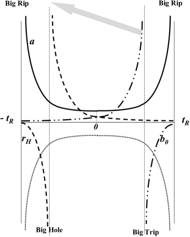
Figure 4: Relative placements along time of the big trip and big hole processes which take place for solution I. It can be observed that whereas a big trip of wormhole occurs on positive time, the big hole of black hole takes place on negative time.

We shall consider in what follows the emergence of big trip events in case of solution II. The rate of change of the wormhole throat radius in the case of a brane symmetric solution ($t_{1}=0$) is

$$\dot{b}=3A\epsilon\rho=\frac{6A\epsilon\lambda}{18\epsilon^{2}\lambda t^{2}-1},$$ (37)

which, after integrating, yields

$$b=\frac{b_{0}}{1-\frac{A\sqrt{2\lambda}b_{0}}{2}\ln\left[\frac{(1-3\sqrt{2\lambda}\epsilon t)((1+3\sqrt{2\lambda}\epsilon t_{0})}{(1+3\sqrt{2\lambda}\epsilon t)(1-3\sqrt{2\lambda}\epsilon t_{0})}\right]}.$$ (38)

The zeros of the denominator of this function would take place at

$$\tilde{t}=\frac{1-\xi}{1+\xi}t_{*},$$ (39)

where $t_{*}=1/(3\sqrt{2\lambda}\epsilon)$ is the absolute value of the time at which the big rips take place, and

$$\xi=\left(\frac{1-\frac{t_{0}}{t_{*}}}{1+\frac{t_{0}}{t_{*}}}\right)e^{2/(A\sqrt{2\lambda}b_{0})}...$$ (40)

It follows that (1) if $0<t_{0}<t_{*}$, $\xi>1$, then there will be a divergent wormhole swelling on $-t_{*}<t<0$ (a situation that also corresponds to $0<|t_{0}|<t_{*}$, with $\xi<0$); (2) if $0<t_{0}<t_{*}$, $0<\xi<1$, then there will be a divergent wormhole swelling on $t_{*}>t>0$; (3) if $t_{0}>t_{*}$, $\xi<0$ $|\xi|>1$, then there will be a divergent wormhole swelling on $t<-t_{*}$ (a situation that also corresponds to $|t_{0}|>t_{*}$, with $\xi<-1$, $|\xi|>1$); and (4) if $t_{0}>t_{*}$, $\xi<0$ $|\xi|<1$, then there will be a divergent wormhole swelling on $t>t_{*}$. Hence, there will be a big trip on every of the possible regions in which the whole time interval running from $-\infty$ to $+\infty$. A similar, but not the same situation is also attained in case that we have a black hole instead of a wormhole. In this case, the rate of change of the black hole mass $M$ due to accretion is

$$\dot{M}=-3B\epsilon\rho=-\frac{6B\epsilon\lambda}{18\epsilon^{2}\lambda t^{2}-1},$$ (41)

with which the following time-dependent black hole mass can be derived

$$M=\frac{M_{0}}{1+\frac{B\sqrt{2\lambda}M_{0}}{2}\ln\left[\frac{(1-3\sqrt{2\lambda}\epsilon t)((1+3\sqrt{2\lambda}\epsilon t_{0})}{(1+3\sqrt{2\lambda}\epsilon t)(1-3\sqrt{2\lambda}\epsilon t_{0})}\right]}.$$ (42)

Thus, $M$ will diverge (big hole) at exactly the times

$$\bar{t}=\frac{1-\eta}{1+\eta}t_{*},$$ (43)

with

$$\eta=\left(\frac{1-\frac{t_{0}}{t_{*}}}{1+\frac{t_{0}}{t_{*}}}\right)e^{-2/(B\sqrt{2\lambda}M_{0})}.$$ (44)

Relative to the distinct observers we obtain in this way a set of possible big holes distributed along the entire interval. The precise pattern of such big holes, together with that for big trips is displayed in Fig. 5. Il will be discussed in the next section how all the regions of the complete time interval can be connected to each other without passing through the big rip singularities. It has been pointed out that, contrary to what is currently observed, braneworld scenarios do not allow the existence of static black hole Maartens . At first sight, this could make the above calculation on black holes irrelevant. However, we are using a kind of nonstatic black holes which might be allowed in braneworlds and, moreover, one can always take our model as an approximation where any kind of black holes can be added.

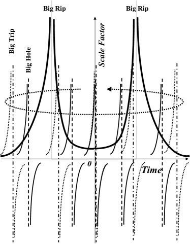
Figure 5: Distribution of the processes of big trip and big hole over the time for solution II. The exact positions will depend on the initial parameters characterizing the corresponding hole, $b_{0}$ for the wormholes and $M_{0}$ for the black holes, and on the time at which the observer is placed.

IV Bridges to the past and future

A Morris-Thorne wormhole can be converted into time machine allowing any object traversing it to time travel into the past or future when the two wormhole mouths are provided with a given relative motion Thorne . Thus, since the space-time where the mouths of such a wormhole are inserted has a given expanding or contracting dynamics, one should expect that a swelling wormhole might behave like a time machine and, when sufficiently grown up, it could even make the swallowed universe and everything in it to time travel as well. It has been in particular shown Gonz1 that during the wormhole swelling induced by phantom energy accretion the chronology protection conjecture Hawking ic violated, so that macroscopic wormholes become quantum-mechanically stable during that accretion process. According to the distinct processes considered in the previous section we can have different kinds of bridges connecting the past and future of the universe, circumventing or not a singularity type big rip, big bang or big crunch. In order to determine the structure and properties of these bridges, we have to take into account two requirements: (1) Any of the space-time swelling processes we have considered in this paper must be described for an asymptotic observer at radial coordinate $r\rightarrow\infty$, for otherwise such processes simply cannot take place or would lead to quite different behaviours Gonz1 , and (2) by their very definition, the spacetime of both a Morris-Thorne wormhole and a black hole ought to be asymptotically flat. This condition makes it impossible that the universe can travel along its own time through a single wormhole. We thus distinguish the following processes.

Single wormhole processes While still smaller than the host universe, the swelling wormhole may allow for given amounts of energy to time travel. Once the wormhole has grown up larger than the cosmological horizon it can no longer insert its mouths into the host universe and, in order to become implanted somewhere, it must necessarily making recourse to other different, sufficiently larger universes, if they are at all available (for example in a multiverse scenario (see Fig. 6)), while satisfying the Israel junction conditions. The lack of a common time for the assumed set of universes would convert the big trip into a simple energy transfer process without any violation of causality. There is thus no proper time travel in the latter case.

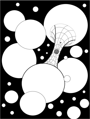
Figure 6: Pictorial representation of the big trip process when it is carried out by a single grown-up wormhole within the framework of a multiverse picture. In this case the universe does not travel along its own time but behaves like though if its whole content were transferred from one different larger universe to another, also larger universe.

Processes induced by a couple of swelling wormholes As a couple of wormholes, one in the past and the other in the future, are growing bigger than the universe in which they are implanted, these wormholes should cease to insert their mouths onto the large regions of the universe where they were originally inserted. The resulting open mouths of one of the wormholes can be then connected to the resulting open mouths of the other, so that the two wormholes turn out to be mutually connected to each other in such a way that they form up a compact, closed quickly inflating tunnel during the while when their throats have grown beyond the size of the cosmological horizon. The universe trapped inside can then flow along the resulting traversable closed tunnel, travelling in this way along its own time (see Fig. 7). This ”big kiss” can always be made to satisfy the Israel junction conditions and therefore effectively allows for the existence of connections between the past and future of the universe. Once the wormholes are annihilated just after the big trip by converting themselves into a couple of black/while hole pairs, the universe would continue its conventional causal evolution, re-starting at the moment it has finished its time travelling.

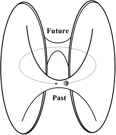
Figure 7: Pictorial representation of the big trip process when two grown-up wormholes are used, one in the past and the other in the future. In this case the two wormhole connect their mouths in such a way that they form a compact tunnel through which the universe can travel along its own time, into the past or future.

Processes induced by the combined action of a swelling wormhole and a swelling black hole The topology resulting in this case is like that of the two swelling wormholes considered in the precedent situation, unless by the feature that one of the two wormholes is replaced for a swelling black hole. The effect is the same, too: the universe can time travel along its own time, this time by using a black hole in the past or future as an intermediate stage on which the wormhole is inserted in a way that also satisfies the junction conditions. At first sight, it could be expected that the black hole would rapidly accrete all the exotic energy that keeps the wormhole throat open, so making impossible this kind of process, but that does not happen in any the cases considered in Sec. III because the black hole swelling takes place only on the branch of time (negative or positive) where its surface gravity becomes always repulsive relative to an observer moving (forward or backward, respectively) in time.

Thus, the question posed at the beginning of Sec. III can be responded in the affirmative. Bridges linking the past and future of the universe may be formed that mark the itineraries of closed timelike curves in a way that is somehow reminiscent to the dream that Gödel kept for most of his late life. Moreover, wormholes by themselves may serve as ways of escaping from the initial and ripping singularities. However, the question of what happens with causality should still be addressed in such a scenario. In fact, the connection between past and future in our universe may lead to time travel paradoxes (TTP); that is, you for example can kill your parents before you were born (grandfather paradox) or you can kill yourself in the past . Could paradoxes like these be avoided in our scenario? There actually are many articles dealing with this matter but the solution is still unclear. For example, Krasnikov Kras has defined time travel paradoxes in physical terms, concluding that no paradoxes arise in general relativity. Another possible way to solve TTP is connected with the many worlds interpretation of quantum mechanics Deutsch , but this solution is faced with its own problems too Everett .

A very attractive solution to the problem of TTP was suggested in Ref. Novikov . For the case of a ”hardsphere” self-interaction potential and wormhole time machines, it was showed that for a particle with fixed initial and final positions traversing the wormhole just once, the only possible trajectories minimizing the classical action are those which are globally self-consistent. The principle of self-consistency (originally introduced by Novikov) becomes thus a natural consequence from the principle of minimal action. Although the verdict is still not settled down on the general validity of this solution (see, for example, Everett ), we shall assume it to be correct. Then it will be shown in what follows that the flatness problem can be solved without making recourse to the inflationary paradigm. In order to understand how this is possible, let us consider the one-particle Schrödinger equation

$$i\hbar\frac{\partial\Psi}{\partial t}=-\frac{\hbar^{2}}{2m}\nabla^{2}\Psi+V\Psi.$$ (45)

Using Bohm substitution Bohm $\Psi=R{\rm e}^{iS/\hbar}$ (with real functions $R$ and $S$) we can obtain two equations. The first one will be just the Hamilton-Jacobi (H-J) equation for a single particle moving in a quantum potential

$$U=V-\frac{\hbar^{2}}{2m}\frac{\nabla^{2}R}{R}.$$

The classical principle of minimal action will hold if $U=V$. In fact, classical mechanics assumes that a particle executes just single paths between two points basing on the minimization of the classical action $S$. In quantum theory all possible paths contribute to the path integral. Thus the principle of minimal action will hold in the present case if $\nabla^{2}R=0$. On the other hand, the latter equation has no bounded nonsingular solutions unless we have $R=$const . The simplest example is the plane waves in nonrelativistic quantum theory. The wave function describes then a free particle.

We can perform a parallel development for the Wheeler-DeWitt equation ${\hat{H}}\psi=0$, where ${\hat{H}}$ is the super-Hamiltonian operator and $\psi$ is the wave function of the universe. Therefore we will have $\psi=R{\rm e}^{iS/\hbar}$, where $R=$const. In other words, $R$ does not depend on the scale factor $a$. Such a non-normalizable wave function of the universe was already suggested by Tipler in Tipler by introducing the boundary condition that the quantum state of the universe should allow Einstein equations to hold exactly in the present epoch. One can therefore conclude that this boundary condition must be satisfied in order to avoid the emergence of TTP in cosmology, provided the conclusion in Novikov is correct. We note however that in the neighborhood of the big rip singularities Einstein equations cannot hold and therefore TTP could then take place.

Moreover, by using a wave function with $R=$const Tipler also showed how the flatness problem can be solved. To see this, let us consider the probability that we will find ourselves in a closed universe with radius larger than any given radius $a_{given}$

$$\int_{a_{given}}^{+\infty}|\psi|^{2}da=+\infty,$$

whereas

$$\int_{0}^{a_{given}}|\psi|^{2}da<+\infty,$$

so the relative probability that we will find ourselves in a universe with radius larger than any given radius $a_{given}$ is one. Thus, using the condition that there are no TTP one can also solve the flatness problem in cosmology.

To make this point clearer let us return to the case of (45). If $V=0$ then the solution of (45) has the form:

$${\Psi={\rm e}^{-i\left(\hbar{\vec{k}}^{2}t/(2m)+{\vec{k}}{\vec{r}}\right)}.}$$ (46)

In the lab we have prior information about initial location of the particle so one must consider wave packet rather then plane wave (46). But if we do not have any (prior) information then we are compelled to use the non-normalizable wave function (46). In this case we cannot calculate the probability $p(V<V_{given})$ to find the particle inside the given volume $V_{given}$ and one can conclude that $p(V<V_{given})\sim V_{given}$. The probability to find this particle out of this volume but inside the volume $V_{1}$ will be proportional to $V_{1}-V_{given}$. Now a relative probability can be obtained exactly:

$$p_{rel}(V<V_{given})=\frac{V_{given}}{V_{1}-V_{given}}.$$

It follows that the relative probability to find the particle inside of the volume $V_{given}$ ($V_{1}\to+\infty$) will be zero and the relative probability to find this particle outside this volume will be one. This is a direct consequence from not having any prior information.

This situation is unusual for the lab but usual for quantum cosmology. In the latter case we do not have any prior information and one need to use the non-normalizable wave function of the universe $\psi$ instead of, say, a wave packet. It is well known that the wave function of the universe is non-normalizable in tree-level approximation and this problem can be solved by including loop effects. But in the framework of our above approach, the wave function in tree-level approximation becomes the true wave function and all loop effects must be suppressed. Our conclusion therefore is that when avoiding time travel paradoxes the way we have outlined above, one finds an extra unexpected reward: the solution of the flatness problem without making any recourse to inflationary ideas.

V Conclusions and further comments

This paper deals with new symmetric cosmological solutions for the late or early universe by using dark energy stuffs that satisfy the energy conditions or violate them in several different ways. The distinctive property of all such solutions is that they can double in a symmetric manner the main singular events predicted by the corresponding quintessential cosmologies. In particular, they make the big rip and the big bang (or big crunch) to appear twice, one on the positive branch of time and the other on the negative one. However the effects of the accretion of this generalized dark energy onto black holes and wormholes do not display such a symmetry so that the big trip only appears once, either on the positive branch or on the negative branch of time. An interesting aspect of our work resides on the possibility of making viable a relevant swelling of black hole space-times so that it may lead to the here dubbed big hole phenomenon by which the black hole grows so big as to swallow the whole universe. That big hole was precluded in quintessence models and is also predicted to appear here just once, either on positive or negative time.

The most interesting sector of the above solutions are derived from the brane world scenario and it is shown that the prediction of a second singular events is a pure brane effect and that the late evolution of the universe predicted in such brane models is due to the existence of an energy density whose absolute value increases with cosmological time, so making most relevant the brane and quantum effects to appear at the latest times. On the other hand, the simultaneous emergence of the big trip and big hole phenomena before and after the cosmic singularities makes it possible to circumvent such singularities so that the full interval for the universe evolution is extended to cover the entire range from $t=-\infty$ to $t=+\infty$.

It should also be remarked that in case that $\epsilon<0$ in the symmetric solution derived from the brane model (solution II), the two symmetric zeros of the scale factor at $t_{\pm}=\pm t_{bb}=1/(3\sqrt{2\lambda}|\epsilon|)$ actually correspond to two big bang (or big crunch) singularities where the energy density diverges. Such singularities can be also circumvented as, similarly to as it happens for positive $\epsilon$, wormhole and black hole swellings and its corresponding big trip and big hole, now taking place at

$$t=T=\frac{\xi-1}{\xi+1}t_{bb},$$ (47)

with

$$\xi=\left(\frac{1+\frac{t_{0}}{t_{bb}}}{1-\frac{t_{0}}{t_{bb}}}\right)e^{2/(A\sqrt{2\lambda}b_{0})}$$ (48)

for wormholes and

$$\xi=\left(\frac{1+\frac{t_{0}}{t_{bb}}}{1-\frac{t_{0}}{t_{bb}}}\right)e^{-2/(B\sqrt{2\lambda}M_{0})}$$ (49)

for black holes, would again crop up along the entire time interval from $-\infty$ to $+\infty$ in such a way that, relative to different observers placed on distinct regions of that interval, there will be no need to pass through the big bang (or big crunch) singularities. This mechanism may provide us with a new alternative for a smooth creation of the universe, other than the Hawking no boundary condition HH or the Gott’s noncausal self-creating condition Gott .

Before closing up, a quite interesting point is worth mentioning. The checked possibility of establishing causality-violating links between the region inside the two big rips and the regions outside that interval for brane solutions (2.12) makes it unavoidable that the space-time to be considered extends from $-\infty$ to $+\infty$ without passing through the big rip singularities. However, for this to be possible it is necessary that the scale factor be well-defined along this infinite interval, a case which can only be satisfied if the parameter $\epsilon$ (or $|\epsilon|$ in case of the solution containing two symmetric big bangs) entering the equation of state is discretized so that Gonz3

$$\epsilon=\frac{1}{12(n+1)},\;\;\;n=0,1,2,3,,\infty.$$ (50)

Even though we do not quite understand yet the deep physical meaning of this requirement one can still say that: (i) it leads to a preliminary ”quantization” of both the involved dynamical quantities such as the energy density, pressure, potential energy and scalar field, and the space-time quantities such as the occurrence time for big bang and crunch, big rip, big trip and big hole, and (ii) it makes any future or past event horizon to disappear, so allowing for any amount of information to be transferred during the big trip process and the formulation of fundamental theories based on the definition of an S-matrix, such as string or M theories, to be mathematically consistent. It is tempting to speculate nevertheless that the discretization of the equation of state parameter could be regarded to be at qualitatively the same footing with respect to a proper quantum theory of the universe as the original Borh theory did in relation with the final probabilistic description of the quantum mechanics of the hydrogen atom.

Although the present work is of a rather speculative nature, all the mathematics and physics involved are rigorously performed and displayed to yield clear results albeit at least some of the interpretations that follow them turn out to be debatable. The authors are therefore suspicious that the conclusions derived in the present paper might play some roles related to subjects such as the final quantum description of the universe and its future evolution.

- (1) Hannestad and E. Mortsell, Phys. Rev. D66 (2002) 063508; M. Tegmark et al. [Collaboration] Phys. Rev. D69 (2004) 103501; U. Seljak et al., Phys. Rev. D71 (2005) 103515; U. Alam et al., Mon. Not. Roy. Astron. Soc. 354 (2004) 275; astro-ph/0406672; D. Huterer and A. Cooray, Phys. Rev. D71 (2005) 023506; B. Feng, X.L. Wang and X.M Zhang, Phys. Lett. B607 (2005) 35; J. Jonsson, A. Goobar, R. Amanullah and L. Bergstrom, JCAP09 (2004) 007. For most recent data on WMAP, see:
- (2) R.R. Caldwell, Phys. Lett. B545 (2002) 23; R.R. Caldwell, M. Kamionkowski and N.N. Weinberg, Phys. Rev. Lett. 91 (2003) 071301; P.F. González-Díaz, Phys. Lett. B586 (2004) 1; Phys. Rev. D69 (2004) 063522; S.M. Carroll, M. Hoffman and M. Trodden, Phys. Rev. D68 (2003) 023509; S. Nojiri and S.D. Odintsov, Phys. Rev. D70 (2004) 103522 .
- (3) P.F. González-Díaz, Phys. Rev. Lett. 93 (2004) 071301; Phys. Lett. B632 (2006) 159; Phys. Lett. B635 (2006) 1.
- (4) S. Perlmutter et al., Nature 391 (1998) 52; A.G. Riess et al. Astron. J. 116 (1998) 1009 .
- (5) B. McInnes, JHEP 0208 (2002) 029; G.W. Gibbons, hep-th/0302199; A.E. Schulz and M.J. White, Phys. Rev. D64 (2001) 043514; J.G. Hao and X. Z. Li, Phys. Rev. D67 (2003) 107303; S. Nojiri and S.D. Odintsov, Phys. Lett.B562 (2003) 147; B565 (2003) 1; B571 (2003) 1; P.Singh, M. Sami and N. Dadhich, Phys. Rev. D68 (2003) 023522; J.G. Hao and X.Z. Li, Phys. Rev. D68 (2003) 043501; 083514; X.Z. Li and J.G. Hao, Phys. Rev. D69 (2004) 107303; M.P. Dabrowski, T. Stachowiak and M. Szydlowski, Phys. Rev. D68 (2003) 067301; M. Szydlowski, A. Krawiec and W. Zaja, Phys. Rev. E72 (2005) 036221; E. Elizalde and J. Quiroga H., Mod. Phys. Lett. A19 (2004) 29; V.B. Johri, Phys. Rev. D70 (2004) 041303; L.P. Chimento and R. Lazkoz, Phys. Rev. Lett. 91 (2003) 211301; H.Q. Lu, Int. J. Mod. Phys. D14 (2005) 355; M. Sami, A. Toporensky, Mod. Phys. Lett A19 (2004) 1509; X.H. Meng and P. Wang, hep-ph/0311070; H. Stefancic, Phys. Lett. B586 (2004) 5; Eur. Phys. J. C36 (2004) 523; D.J. Liu and X.Z. Li, Phys. Rev. D68 (2003) 067301; A. Yurov, astro-ph/0305019; Y.S. Piao and E. Zhou, Phys. Rev. D68 (2003) 083515; Y.S. Piao and Y.Z. Zhang, Phys. Rev. D70 (2004) 063513; J.M. Aguirregabiria, L.P. Cimento and R. Lazkoz, gr-qc/0403157; J. Cepa, Astron. Astrophys. 422 (2004) 831; V. Faraoni, Phys. Rev. D69 (2004) 123520; Z.-K. Guo, Y.-S. Piao and Y.-Z. Zhang, Phys. Lett. B606 (2005) 7; E. Elizalde, S. Nojiri and S. Odintsov, Phys. Rev. D70 (2004) 043539; Y.-H. Wei and Y. Tian, Class. Quant. Grav. 21 (2004) 5347; F. Piazza and S. Tsujikawa, JCAP 0407 (2004) 004 .
- (6) P.F. González-Díaz and J.A. Jiménez Madrid, Phys. Lett. B596 (2004) 16.
- (7) F.S.N. Lobo, Phys. Rev. D71 (2005) 084011 .
- (8) P. Martín-Moruno, J.A. Jiménez Madrid and P.F. González-Díaz, astro-ph/0603761 .
- (9) A.V. Yurov, S. D. Vereshchagin, Theor. Math. Phys. 139 (2004) 787-800 [hep-th/0502099].
- (10) L. Randall and R. Sundrum, Phys. Rev. Lett. 83 (1999) 4690 .
- (11) S. V. Krasnikov, gr-qc/0603060.
- (12) S.V. Krasnikov, Phys. Rev. D57 (1998) 4760.
- (13) A.E. Everett and T.A. Roman, Phys. Rev. D56 (1997) 2100.
- (14) L. H. Ford and T. A. Roman, Phys. Rev. D53 (1996) 5496.
- (15) L. H. Ford, M. J. Pfenning, and T. A. Roman, Phys. Rev. D57 (1998) 4839.
- (16) D. N. Vollick, Phys. Rev. D61 (2000) 084022.; E. E. Flanagan. ibid. V. 66. (2002) 104007.
- (17) C. J. Fewster, Phys. Rev. D70 (2004) 127501.
- (18) M. J. Pfenning and L. H. Ford, Class. Quantum Grav. V. 14. (1997) P. 1743.
- (19) K. Gödel, Rev. Mod. Phys. 21 (1949) 447 .
- (20) D. Bohm, Phys. Rev. 84 (1951) 166; 85 (1952) 180.
- (21) E. Babichev, V. Dokuchaev and Yu. Eroshenko, Phys. Rev. Lett. 93 (2004) 021102.
- (22) R. Maartens, Living Rev. Rel.7 (2004) 7 .
- (23) M.S. Morris, K.S. Thorne and M. Yursever, Phys. Rev. Lett. 61 (1988) 1446; M.S. Morris and K.S. Thorne, Am. J. Phys. 56 (1988) 395.
- (24) S.W. Hawking, Phys. Rev. D46 (1992) 603.
- (25) S. Krasnikov, Phys. Rev. D65 (2002) 064013.
- (26) D. Deutsch, Phys. Rev. D44 (1991) 3197; Sci. Amer. March (1994) p. 68.
- (27) Allen Everett, Phys. Rev. D69 (2004) 124023.
- (28) A. Carlini, V.P. Frolov, M.B. Mensky, I.D. Novikov, H.H. Soleng, Int.J.Mod.Phys. D5 (1996) 445-480.
- (29) Frank J. Tipler, astro-ph/0111520.
- (30) J. B. Hartle and S.W. Hawking, Phys. Rev. D28 (1983) 2960 .
- (31) J.R. Gott and Li-Xin Li, Phys. Rev. D58 (1998) 023501 .
- (32) P.F. González-Díaz, Grav. Cosm. 12 (2006) 29 .