Contour binning: a new technique for spatially-resolved X-ray spectroscopy applied to Cassiopeia A

Abstract

We present a new technique for choosing spatial regions for X-ray spectroscopy, called “contour binning”. The method chooses regions by following contours on a smoothed image of the object. In addition we re-explore a simple method for adaptively smoothing X-ray images according to the local count rate, we term “accumulative smoothing”, which is a generalisation of the method used by fadapt. The algorithms are tested by applying them to a simulated cluster data set. We illustrate the techniques by using them on a 50 ks Chandra observation of the Cassiopeia A supernova remnant. Generated maps of the object showing abundances in eight different elements, absorbing column density, temperature, ionisation timescale and velocity are presented. Tests show that contour binning reproduces surface brightness considerably better than other methods. It is particularly suited to objects with detailed spatial structure such as supernova remnants and the cores of galaxy clusters, producing aesthetically pleasing results.

1 Introduction

Many X-ray telescopes such as XMM-Newton, Chandra and ROSAT contain detectors which capture individual photons, recording their energy and position on the detector. Therefore unlike conventional optical observing techniques, we simultaneously collect imaging and spectroscopic data for each part of the object. In addition the Chandra X-ray Observatory has very high spatial resolution ($\sim 1$ arcsec), allowing the properties of the emitting object to be studied in unprecedented detail.

With this spectroscopic and imaging information we can select “events” from the observation corresponding to a particular part of an object with a “region filter”. From these events a spectrum can be built-up. An X-ray spectral package such as xspec (Arnaud 1996) can then be used to fit a physical model to the spectrum. Conventionally simple geometric shapes such as annuli, sectors, boxes or ellipses are used to define a region filter. Using sectors, for example, and assuming spherical or elliptical symmetry, one can account for projection in a cluster of galaxies. However most extended objects are not symmetric when observed in detail (for example, the Perseus cluster [Fabian et al 2000; Sanders et al 2004], the Cassiopeia-A supernova remnant [Hwang et al 2004], and Abell 2052 [Blanton, Sarazin & McNamara 2003]).

Given the morphological diversity of extended X-ray sources it is important to have techniques which allow us to analyse the spectral variation of a source over its extent. We first investigated this problem when looking for cool gas in a sample of X-ray clusters using ROSAT PSPC archival data (Sanders, Fabian and Allen 2000). We devised a technique which used adaptively smoothed maps (Ebeling et al, in preparation) to define contours in surface brightness. The ratio of the number of counts in different energy bands between each contour was used to define an X-ray colour. By using a grid of models, the absorption and temperature of the gas could be estimated between the contours.

We approached this problem again with the advent of data from Chandra with its high spatial resolution. We created an algorithm called “adaptive binning” (Sanders & Fabian 2001) which used the uncertainty on the number of counts or the error on the ratio of counts in different bands to define the size of binning region used. The process was simple: pass over the image, copying those pixels which have a small enough uncertainty on the number of counts or colour to an output image. Bin up the remaining pixels by a factor of two. Repeat until all the pixels have been binned. On the final pass we bin any pixels which are not yet binned. This simple approach works well and was used by us and other authors on data from several clusters of galaxies (e.g. Centaurus – Sanders & Fabian 2002; Perseus – Fabian et al 2000; Abell 4059 — Choi et al 2004).

The disadvantage of this approach is that the binning scale varies by factors of two. It is very noticeable where the scale changes, and some regions are overbinned. Therefore we started using the “bin accretion” algorithm of Cappellari & Copin (2003). The algorithm adds pixels to a bin until a signal-to-noise threshold is reached. After all the pixels have been accreted, it uses Voronoi tessellation to make tessellated regions based on the weighted position of the original bins. This technique has the advantage of creating bins which are compact, varying in size smoothly with the surface brightness, and also provides bins with similar signal-to-noise ratios. We applied the method to X-ray observations of the Perseus cluster (Sanders et al 2004) and Abell 2199 (Johnstone et al 2002). Rather than use X-ray colours, we extracted spectra for each of the regions and used spectral fitting to derive, for example, temperature and abundance maps. Recently Diehl & Statler (2006) have generalised this algorithm to allow for data whose signal-to-noise does not add in quadrature.

The motivation for further work in this area is that the methods above do not use the surface brightness distribution to change the shape of each bin. Physical parameters (e.g. density, temperature and abundance) usually change in the direction of surface brightness changes. The method we describe here uses the surface brightness to define bins which cover regions of similar brightness.

Other methods have been presented for mapping the parameters of the intracluster medium. These included wavelet techniques (Bourdin et al 2004) and monte carlo methods (Peterson, Jernigan & Kahn 2004). The advantage of binning techniques is that they provide errors on individual spectral fit parameters, or colours, from a particular part of the sky. The individual measurements made using binning methods are independent, making it easy to easily measure the significance of individual spatial features.

The techniques presented in this paper have already been applied to a number of Chandra observations of clusters, including a deep observation of the complex structure of the Centaurus cluster (Fabian et al 2005), the possible detection of nonthermal radiation and the identification of a high metal shell likely to be associated with a fossil radio bubble in the Perseus cluster (Sanders et al 2005), a sample of moderate redshift clusters (Bauer et al 2005), and a 900 ks observation of the Perseus cluster (Fabian et al 2006), finding little evidence for temperature changes associated with shock-like features, and producing evidence of a substantial reservoir of cool X-ray emitting material.

We first present a simple smoothing method (“accumulative smoothing”), and then present the binning method based on the smoothed image (“contour binning”).

2 Accumulative smoothing

In order to bin using the surface brightness it was necessary for us to get an estimate of the surface brightness in an image in the absence of noise and counting statistics. Simple Gaussian smoothing can be sufficient, but if the brightness of the object varies over its extent the smoothing scale will be too small or too large in parts of the image. There are several methods for adaptively smoothing an image based on the surface brightness (e.g. asmooth, Ebeling et al, in preparation; csmooth in ciao, based on asmooth; Huang & Sarazin 1996). We present a method called accumulative smoothing, which is a generalisation of the method used by the ftools routine fadapt, now including handling background and exposure variation. In addition we adapt the method to create smoothed colour maps. This smoothing method has the advantage of being fast, simple and easy to interpret. It allows the use of blank-sky background images (rather than trying to estimate the local background), masks, and exposure maps. Its disadvantage is that it does not guarantee to globally preserve counts. This is probably not a serious problem as it is usually more important to preserve the local count rate. We will discuss how well it does locally later.

It is a very simple routine which smooths an image with a top-hat kernel, whose size varies as a function of position. The size is varied so that the kernel contains a minimum signal-to-noise ratio.

Suppose there is an input image I, containing numbers of counts in each pixel There is also a background image B (optionally fixed to zero). The smoothed count image at positions $\mathbf{r}$, where $\mathbf{r}$ is a vector representing the coordinates of the centre of the pixel being examined, is

$$\textbf{{S}}(\mathbf{r})=\frac{1}{N}\sum_{|\mathbf{a}-\mathbf{r}|\leq R(\mathbf{r})}{\left[\textbf{{I}}(\mathbf{a})-\frac{E_{i}}{E_{b}}\textbf{{B}}(\mathbf{a})\right]},$$ (1)

where $N$ is the number of pixels summed over ($\sim\pi R[\mathbf{r}]^{2}$), and the smoothing radius at the pixel, $R(\mathbf{r})$, is defined in Equation 3. $E_{b}$ and $E_{i}$ are the exposure times of the foreground and background observations, respectively. If we wish to take account of the variation in exposure times over an image, we can create a smoothed count rate image,

$$\textbf{{S}}_{\mathrm{rate}}(\mathbf{r})=\frac{1}{N}\sum_{|\mathbf{a}-\mathbf{r}|\leq R(\mathbf{r})}{\left[\frac{\textbf{{I}}(\mathbf{a})}{E_{i}(\mathbf{a})}-\frac{\textbf{{B}}(\mathbf{a})}{E_{b}(\mathbf{a})}\right]},$$ (2)

The smoothing radius $R(\mathbf{r})$ is defined to be the minimum value of the radius (in integer units) where the signal-to-noise is greater or equal to a threshold value. Summing over pixels at positions $\mathbf{a}$, where $|\mathbf{a}-\mathbf{r}|\leq R(\mathbf{r})$, then the condition is met when

$$[S/N](\mathbf{r})\sim\frac{\sum\left[\textbf{{I}}(\mathbf{a})-\frac{E_{i}(\mathbf{a})}{E_{b}(\mathbf{a})}\textbf{{B}}(\mathbf{a})\right]}{\left(g\left[\sum\textbf{{I}}(\mathbf{a})\right]+\frac{1}{N}\sum\left\{\left[\frac{E_{i}(\mathbf{a})}{E_{b}(\mathbf{a})}\right]^{2}\right\}g\left[\sum\textbf{{B}}(\mathbf{a})\right]\right)^{1/2}}\geq M.$$ (3)

$R(\mathbf{r})$ is found by incrementing $R(\mathbf{r})$ from 1 until it is true. $g(c)$ is an approximation for the squared-uncertainty on $c$ counts, obtained from equation 7 of Gehrels (1986) when $S=1$,

$$g(c)=\left(1+\sqrt{c+\frac{3}{4}}\right)^{2}.$$ (4)

This approximation is the larger error bar on $c$ counts, so we overestimate the negative error by assuming the errors are symmetric.

Equation 3 is approximate if the ratio of the exposure time of the image and background varies over the image. We do not sum the squared error of $\textbf{{B}}(a)$ as the sum of the approximation for the uncertainty squared $g(c)$ will become increasingly inaccurate with more terms.

Therefore the algorithm smooths the image using a top-hat kernel with a variable smoothing radius. The smoothing radius varies so that it contains a minimum signal-to-noise ratio. We handle edges and masked regions by ignoring pixels outside the valid region ($N$ does not include these pixels).

2.1 Tests of the algorithm

To test how closely the smoothing algorithm reproduces the surface brightness of a model image, we constructed a surface brightness model made up of six $\beta$ surface brightness model components, where each component had surface brightness

$$S=S_{0}\left(1+\left[\frac{r}{r_{c}}\right]^{2}\right)^{-3\beta+1/2}.$$ (5)

The components are listed in Table 1. We constructed a model $512\times 512$ pixel image based on the components (Fig. 1 [left]). A Poisson statistic realisation of the model is shown in Fig. 1 (centre). In Fig. 1 (right) we include an accumulatively smoothed image of the Poisson realisation.

$S_{0}$ (counts)	$\beta$	$r_{c}$ (fraction)	$x_{c}$ (fraction)	$y_{c}$ (fraction)
40	0.67	1/4	1/2	1/2
40	0.67	1/16	1/4	1/4
40	1	1/64	1/4	3/4
40	5	1/64	0.8	0.5
8	0.67	1/16	0.9	0.1
-12	0.67	1/16	0.65	0.65

Table 1: Surface brightness components. Each is a $\beta$ surface brightness model (Equation 5). The core radius ($r_{c}$), component $x$ centre ($x_{c}$) and $y$ centre ($y_{c}$) are expressed as a fraction of the $512\times 512$ pixel image. The coordinates are measured from the lower left of the images.

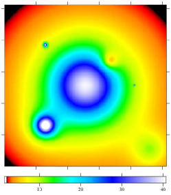
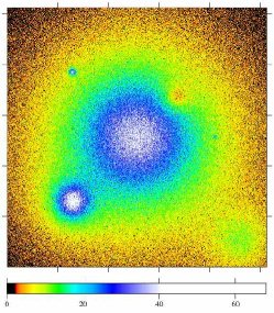
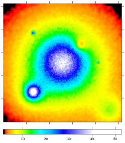
Figure 1: (Left) Surface brightness model made up of six $\beta$ model components. (Middle) Realisation of the model assuming Poisson statistics. (Right) Accumulatively smoothed image of the realisation, with a signal-to-noise ratio of 20. All three images use the same colour scale. The units are counts per pixel.

A good smoothing algorithm should reproduce the model image with no large scale deviations or biases, and random small scale deviations. We computed the fractional difference between smoothed images of the realisation of the model with various signal-to-noise threshold ratios (Fig. 2). Also shown is a Gaussian smoothed fractional difference map for comparison. To aid comparison we show histograms of the fractional differences using accumulative smoothing and Gaussian smoothing with different signal-to-noise ratios and scale lengths in Fig. 3.

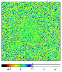
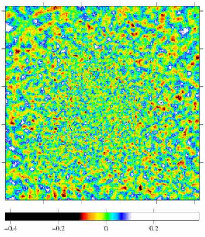
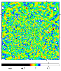
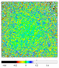
Figure 2: Fractional difference between complex cluster model and accumulatively-smoothed image, for $S/N$ 8, 20 and 30, and using Gaussian smoothing with a smoothing scale of 2 pixels. Note that each image uses a different colour scale to show the magnitude of the scatter.

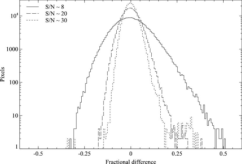
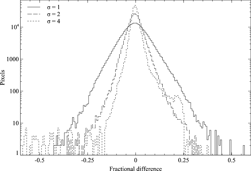
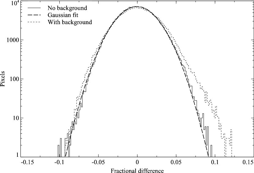
Figure 3: Histogram of fractional differences between reconstructed surface brightness and original model. (Top) Difference between complex cluster model and accumulatively-smoothed data. The three curves are smoothed with signal-to-noise threshold ratios of 30, 20 and 8. (Centre) Fractional difference between the model and Gaussian-smoothed data (using widths of 1, 2 and 4 pixels). (Bottom) Differences between a single-component $\beta$ model and accumulative smoothed data (signal-to-noise threshold of 40). The smooth line is a Gaussian fit to the differences, with a best fitting width of 0.023. The edges of the image have been removed to eliminate edge effects. Also plotted is the result when a constant background is added to the model.

Firstly, accumulative smoothing mostly shows deviations from the model which do not vary in magnitude over the image. The Gaussian smoothed deviations in Fig. 2 (right) increase when the count rate decreases. The central part of the image is uniform in colour, while the outer parts alternate between the extremes. Where accumulative smoothing shows deviations are at the edge of the image and around centrally-concentrated sources when the smoothing scale is too large (e.g. Fig. 2 [centre right]). Near the edges the surface brightness is too high, as there are no lower flux pixels further out to smooth over. If a centrally-concentrated source does not have enough signal to exceed the signal-to-noise threshold, $M$, then it is smoothed into its surroundings. The flux at the centre of the source is underestimated, and the flux in its surroundings is overestimated.

We took a single $\beta$ component surface brightness image (using an image of size $1024\times 1024$ pixels, and applied Gaussian ($\sigma=8$ pixels using the fgauss program from ftools) and accumulative smoothing ($M=40$) to a Poisson realisation of the model. In the centre of the image, the Gaussian smoothing length is approximately the accumulative smoothing length.

The deviation distributions (Fig. 3) show that accumulative smoothing produces narrower tails in the distribution than Gaussian smoothing. The distributions can be well fit with a Gaussian, except for a tail in the positive deviations. At low signal-to-noise thresholds this may be due to the approximation in the uncertainties of the counts as symmetric. The Gehrels approximation used overestimates the uncertainty on low numbers of counts, meaning that faint regions will have larger kernels applied than necessary when a low signal-to-noise threshold is used. At high signal-to-noise the tail is due to edge effects and oversmoothed compact sources. Using a model distribution that contains just the central $\beta$ component, and excluding the edges of the image, produces a distribution which is almost Gaussian (Fig. 3 [bottom]). The width of the distribution is 0.023, which is very close to a simple estimation of the width ($1/M=0.025$). To get the estimate, we require $c=M^{2}$ counts in the absence of a background to exceed the threshold. The standard deviation on a mean of $c$ counts is $\sqrt{c}$, or as a fraction of the mean, $1/\sqrt{c}=1/M$.

We have also considered the case of a simple $\beta$ model with a background. We added a background of 40 counts across the entire image (which is the same as the peak of the $\beta$ distribution). The distribution of deviations (Fig. 3 [bottom]) is fairly Gaussian, although there is a significant tail at larger deviations than the case without a background. In this test we assumed the background was very well determined (simulated by using a much larger exposure time for the background than the foreground).

2.2 Colour maps

Colour maps show the ratio of counts in two bands. Such maps are useful because trends in X-ray colour can follow physical trends (e.g. temperature or absorption). Accumulative smoothing can also be used to generate smoothed colour maps. Smoothing or binning is very useful in creating colour maps, as the error on a ratio of two counts can greatly vary over an X-ray image.

Rather than considering a threshold on the signal-to-noise in the smoothing kernel, a maximum uncertainty on the X-ray colour can be used instead.

2.3 Conclusions

It can be concluded that accumulative smoothing, and the smoothing of fadapt when there is no background or exposure variation, does not introduce a major bias to an image. The median difference is negligible for all three smoothing thresholds shown. Accumulative smoothing is certainly better than Gaussian smoothing at smoothing on appropriate scales over an image. Indeed the deviation range does not change with position. It also produces a distribution of deviations that shows a narrow, almost Gaussian, tail, although the tail is wider for positive deviations at low signal-to-noise. If there is not enough signal in point sources they are smoothed into their surroundings, leading to deviations from the intrinsic surface brightness of the sky. In comparison Gaussian smoothing shows much more noise in regions where the count rate is low compared to where it is high.

In addition the algorithm is particularly suited for presentation of X-ray images as an alternative to Gaussian smoothing. It may well be better in many cases to other forms of adaptive smoothing as it introduces few artifacts.

3 Contour binning

Here we describe how the accumulatively smoothed map can be used to define independent spatial regions. These regions can be used for spectral extraction and fitting, to measure physical parameters, or for the calculation of X-ray colours. The method need not apply to accumulatively smoothed images. Other techniques such as adaptive smoothing could be used instead.

Simply, the algorithm, starting at the highest flux pixel on a smoothed image, adds pixels nearest in surface brightness to a bin until the signal-to-noise ratio exceeds a threshold algorithm. A new bin is then created. This technique naturally creates bins which follow the surface brightness.

3.1 Initial pass

Contour binning takes the smoothed image, $\textbf{{S}}(\mathbf{r})$. We start from the highest flux pixel in the smoothed image. The pixel is added to the set of pixels in the current bin, $\beta$. If the signal-to-noise of the pixels in $\beta$ is greater or equal than a binning threshold $T$,

$$[S/N]_{\beta}\sim\frac{\sum_{\mathbf{a}\in\beta}{\left[\textbf{{I}}(\mathbf{a})-\frac{E_{i}(\mathbf{a})}{E_{b}(\mathbf{a})}\textbf{{B}}(\mathbf{a})\right]}}{\left(\sum_{\mathbf{a}\in\beta}{\left\{g[\textbf{{I}}(\mathbf{a})]+\left[\frac{E_{i}(\mathbf{a})}{E_{b}(\mathbf{a})}\right]^{2}g[\textbf{{B}}(\mathbf{a})]\right\}}\right)^{1/2}}\geq T,$$ (6)

then the region is complete. Otherwise we iterate over the subset of $\beta$ which lie at the edge of the bin. We consider all the unbinned neighbours of these pixels and take the one which has a flux in the smoothed image closest to the starting flux of the bin. This pixel is added to $\beta$, and we repeat the process. If there are no neighbouring unbinned pixels we stop this bin. We consider a pixel to be a neighbour if it differs in one of its coordinates by 1, and in the others by 0 (diagonally neighbouring pixels could also be included, however).

Once we have completed the bin, we start binning again. The starting pixel is again the highest flux pixel in the smoothed image which has not yet been binned. To optimise this potentially expensive search, we sort the pixels in the smoothed image into flux order before binning.

3.2 Cleaning pass

After all the pixels have been binned, there will be some bins with a signal-to-noise ratio of less than $T$. Many of these will contain single pixels which were left stranded between other bins. The number of these stranded bins decreases with increased smoothing of the initial image. We therefore “clean up” the bins to remove any below the threshold. We start by selecting the bin with the lowest signal-to-noise ratio. By examining its edge pixels, we select the pixel which is closest in smoothed value to a pixel in a neighbouring bin. This pixel is moved into the corresponding neighbouring bin (thereby increasing the signal-to-noise ratio of its neighbour). We repeat, transferring the pixels until there are no pixels remaining in the lowest signal-to-noise bin. We move onto the next remaining bin which has the lowest signal-to-noise and repeat the whole process. The cleaning pass ends when there are no more bins with a signal-to-noise ratio of less than the threshold $T$.

3.3 Constraints

On a high signal-to-noise dataset with low signal-to-noise bins the above process is sufficient. However there are possible undesirable features under other conditions. If the smoothed map is not very smooth, the bins can become distended (this can be improved at the detriment of potential detail by increasing $M$). If the smoothed map is very smooth and radial, then bins will become whole annuli if $T$ is too large. In some cases this outcome is desirable.

To prevent these problems we can impose extra geometric constraints during the binning process. Ideally such a constraint could be computed in constant time on each iteration or else growing large bins becomes prohibitively expensive. We identified a fast constraint that gave the most aesthetic results. The procedure is to estimate a radius $R$ that the current bin would have if it were a circle, i.e. $R\sim\sqrt{N/\pi}$, where $N$ is the number of pixels in the bin. By examining circles on a pixelated grid, we calculate this value exactly for integer radii. This is far better than the simple estimate for small circles. We then measure the distance $d$ of the pixel to be added from the current flux-weighted centroid of the bin. If $R/d>C$, where $C$ is the constraint parameter, then we do not add the pixel. The constraint is also applied during the cleaning pass by moving pixels into only bins in which the constraint would be satisfied. If there are no bins which would satisfy the constraint, the constraint is broken to prevent isolated pixels.

3.4 Tests of the algorithm

We binned the simulated image in Fig. 1 with the algorithm. Fig. 4 shows the image binned using a signal-to-noise ratio, $T$ threshold of 30 and 100 (smoothing with ratios, $M$, of 15 and 40, respectively). The $T=100$ image has also had a constraint of $C=2$ applied. We also show a binned image using a signal-to-noise ratio of 100 using the bin-accretion algorithm of Cappellari & Copin (2003), and simple adaptive binning (Sanders & Fabian 2002) for comparison. The contour binning method appears to give a good reconstruction of the surface brightness. Using the same signal-to-noise ratio, it follows the surface brightness contours better than the tessellated image.

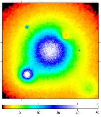
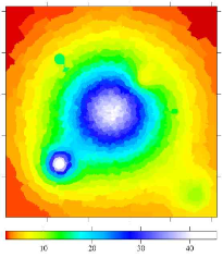
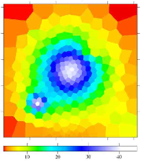
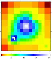
Figure 4: (Left) Contour binned surface brightness image with $T=30$, $M=15$. (Centre Left) Contour binned image with $T=100$, $M=40$ and constraint $C=2$ applied. (Centre Right) Image created using bin-accretion algorithm of Cappellari & Copin (2003) with signal-to-noise ratio of 100. (Right) Adaptively binned image (Sanders & Fabian 2001) with a fractional error of 0.01 (equivalent to a signal-to-noise ratio of 100). All images have units of counts per pixel and the colour scales are the same as in Fig. 1.

In Fig. 5 we show absolute fractional difference maps between the binned images in Fig. 4 and the model map (Fig. 1 left). The comparison between the contour binning and bin accretion methods is not completely fair, as the contour binning procedure uses a minimum signal-to-noise ratio of 100, whilst bin accretion uses a mean signal-to-noise ratio of 100. However increasing the signal-to-noise ratio used by the bin accretion method would increase the size of the bins further.

The signal-to-noise ratio of the bin accretion method can be adjusted to give almost the same number of bins as contour binning. The distribution of the deviations of pixels from the model are shown for the three methods in Fig. 6. The plot shows that contour binning produces values which are considerably closer to the model distribution than the other methods, due to its method of grouping together pixels with the similar values.

For contour binning, the deviations appear random over the bins, except for the two peaked sources with large signal-to-noise ratios. In Fig. 7 is shown the distribution of the fractional differences between the binned surface brightness map and the model map for the contour binned images shown, plus another with $T=10$. The plots show the the differences are close to Gaussian. At the low signal-to-noise ratio of 10 there is some asymmetry in the distribution towards higher fractional differences. This may be due to the use of the Gehrels approximation for the Poisson errors. The width of the distributions is close to the estimated value of $1/T$. The estimated width of the distribution is the same as at the end of Section 2.1. $c=T^{2}$ counts are required to exceed the threshold without a background. The standard deviation on a mean of $c$ counts is $\sqrt{c}$. If this is turned into a fractional width of the distribution it equals $1/\sqrt{c}=1/T$.

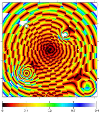
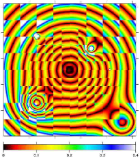
Figure 5: Absolute fractional differences between binned surface brightness image and model image. The panels shown are the same binning as Fig. 4

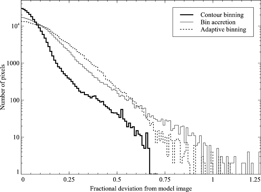
Figure 6: Plot of the distribution of absolute deviation of binned pixels from the model values for similar signal-to-noise ratios. The contour binning and adaptive binning values were taken from Fig. 5 (centre left and far right panels). The signal-to-noise ratio of the bin accretion used has been adjusted from 100 to 106 to get a similar number of bins compared to the contour binning results (257 versus 255). This makes little difference to the distribution. The plot shows that contour binned surface brightness is closer to the model surface brightness than the other methods.

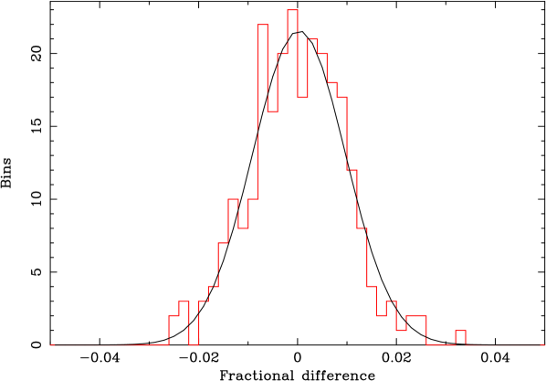
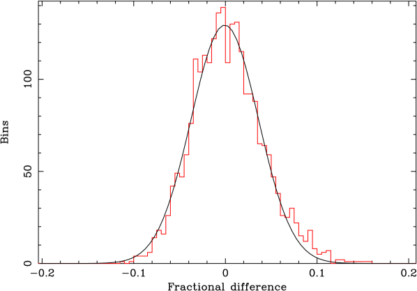
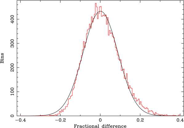
Figure 7: Distribution of fractional difference between the binned surface brightness of a bin and the mean model surface brightness in the bin. The smooth curve is a best fitting Gaussian. (Top) Fractional differences for $T=100$, $M=40$, constraint applied with $C=2$. Best-fitting Gaussian centre is $3.0\times 10^{-4}$, width is $9.4\times 10^{-3}$ (Centre) $T=30$, $M=15$. Gaussian parameters of ($-6.8\times 10^{-4}$, 0.037) (Bottom) $T=10$, $M=15$. Gaussian parameters of ($1.3\times 10^{-3}$, 0.087).

3.5 Spectral fitting tests

To thoroughly test the algorithm when using it to define regions to perform spectral extraction and fitting on, we constructed simulated Chandra event files for a cluster of galaxies. To produce the files, we iterated over cells in a 3-dimensional cube of dimensions $500\times 500\times 1000$ pixels, using a cell size in $(x,y,z)$ of 2, 2 and 4 pixels. In each cell we used xspec to fake a PI (pulse-invariant) spectrum corresponding to the gas in the cluster that would be in that cell. To do this we use an analytical form of the temperature, density and abundance of the gas as a function of radius. The density is used to calculate the emission measure, and the spectrum is faked using the mekal spectral model (Mewe, Gronenschild & van den Oord 1985; Liedahl, Osterheld & Goldstein 1995), with Galactic photoelectric absorption.

We added the spectra along each line of sight in $z$ to produce a 2-dimensional set of spectra. For each spectrum, we manufactured faked events which would produce the spectrum if it were extracted from the $2\times 2$ pixel projected cell on the sky. The events were randomised in position over the projected cell.

In detail, a template event file from a real Chandra observation was populated with these events. To create the faked spectra a constant response and ancillary-response was used in each cell. We used a response for the centre of the ACIS-S3 CCD in 2000. The spectra were faked for an observation of 60 ks. In addition to the emission of the cluster in each cell on the sky, we added events which would produce a background spectrum corresponding to the spectrum observed from a blank-sky observation (generated by fitting a three-component power law model to spectra from a blank-sky background field).

To model the emission from a cluster, we fitted analytic models to the deprojected temperature, density and abundance profiles measured in Abell 2204 (Sanders, Fabian and Taylor 2005a). The cluster was centred in the centre of the cube, and the properties of the gas at each radius in the cluster was found using the analytic fits to the A2204 profiles.

The density profile in A2204 was fitted with a $\beta$ density model of functional form

$$n_{e}(r)=n_{0}\left[1+\left(\frac{r}{r_{c}}\right)^{2}\right]^{-3\beta/2},$$ (7)

with $r_{c}=13.97\rm\thinspace kpc$, $n_{0}=0.1978\hbox{$\rm\thinspace cm^{-3}\,$}$ and $\beta=0.465$. The temperature was modelled with

$$T(r)=T_{0}+\>T_{1}\frac{(r/r_{c})^{\eta}}{1+(r/r_{c})^{\eta}},$$ (8)

with $T_{0}=2.98\rm\thinspace keV$, $T_{1}=7.38\rm\thinspace keV$, $r_{c}=50.2\rm\thinspace kpc$ and $\eta=2.97$. The abundance was modelled with the same functional form, with $Z_{0}=0.156\hbox{$\thinspace\mathrm{Z}_{\odot}$}$, $Z_{1}=0.921$, $r_{c}=47.8\rm\thinspace kpc$, and $\eta=-7.56$. The simulated cluster was assumed to lie at a redshift of 0.15, and we used a cosmology of $H_{0}=70\hbox{$\hbox{$\rm\thinspace km\rm\thinspace s^{-1}\,$}\rm\thinspace Mpc^{-1}$}$ and $\Omega_{\Lambda}=0.7$. Using Chandra pixel sizes, 1 pixel corresponds to 1.28 kpc for the real cluster.

Using the faked dataset, we created an image of the simulated cluster, and of the simulated background, in the 0.5 to 7.0 keV band. This was contour binned using a signal-to-noise of 75 ($\sim 5600$ counts), smoothing the image with a signal-to-noise of 20, and constraining the bins using a parameter $C=2$ (see Section 3.3). This procedure yielded 52 bins in total.

Individual spectra were extracted from the dataset using the regions defined by each bin, and each spectrum was fitted with a mekal model with free absorption, metallicity, temperature and normalisation. The spectra were fit between 0.5 and 7 keV, minimising the $\chi^{2}$ statistic. We show the resulting maps in Fig. 8, whilst radial profiles are shown in Fig. 9.

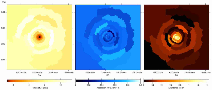
Figure 8: Resulting emission weighted temperature, photoelectric absorption and abundance maps generated from the simulated cluster. Each region was created to have a minimum signal-to-noise ratio of 75. Fig. 9 shows the extracted radial profiles.

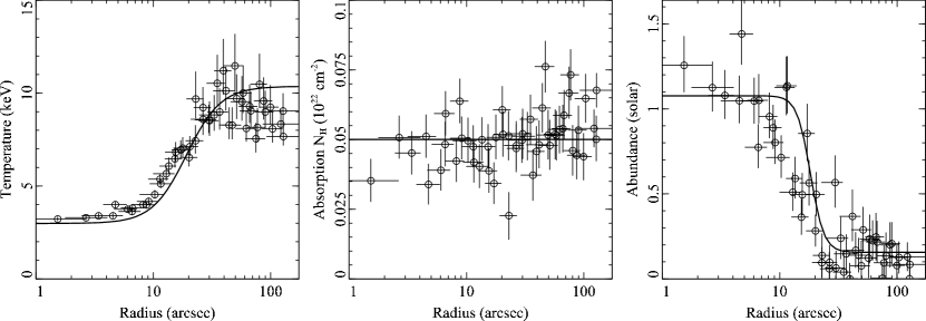
Figure 9: Profiles produced by fitting bins with a minimum signal-to-noise ratio of 75 using the faked data. (Left) temperature, (centre) photoelectric absorption and (right) abundance. The solid lines show the intrinsic (not projected) profiles the faked data was generated with.

The results show the accumulative binning algorithm does a reasonable job at reproducing the input profiles. They do demonstrate some deviations which are due to projection effects, and emission weighting, however. Any method which does not account for projection will be susceptible to these problems. In particular the cool gas in the centre is measured to be too hot. This is due to the projection of the hotter gas outside this region. To account for projection, you must assume some sort of symmetry.

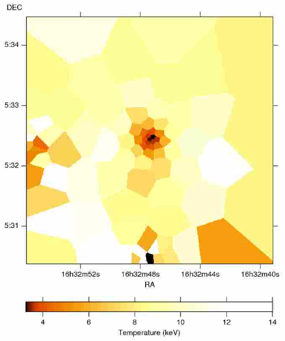
Figure 10: Temperature map created by applying bin accretion algorithm to fake data.

As a comparison, Fig. 10 shows the temperature map from the data binned using the bin accretion algorithm, with the same signal-to-noise ratio. In the central region the bins are not as well shaped to match the surface brightness, leading to a blocky appearance. There are some problems with small bins being generated in the outskirts of the image, but it is possible this could be due to problems in our implementation of the algorithm. Again the comparison is not quite fair as bin accretion uses a mean signal-to-nose ratio, rather than a minimum one. However, increasing the signal-to-noise ratio would make the bins larger.

4 Cassiopeia A

Cassiopeia A is a very good target to demonstrate the algorithm on. The large range in brightness of the image between the bright knots and the darker regions shows off the advantages of this particular method. We present here results using a 49.7 ks observation of Cas A using the ACIS-S3 detector on Chandra taken on 2002-02-06 (observation number 1952).

4.1 Data preparation

Firstly we reprocessed the level 1 event file using ciao 3.3.0.1 with the gain file acisD2000-08-12gainN0005.fits. Time dependent gain correction was also applied using the corr_tgain utility using the November 2003 correction (Vikhlinin 2003). In addition the ciao version of the lc_clean script (Markevitch 2004) was used to remove periods of the dataset where the count rate was 20 per cent away from the mean. Very little time was removed, producing a level 2 event file with an exposure of 48.3 ks, although such filtering is difficult on such a bright target.

The dataset was taken using the unusual GRADED observation mode of the ACIS detector, where events likely to be background are discarded at the satellite rather than removed by the observer. Despite this, the background rate at high energy (9 keV or more) matches that from blank sky observations. We used a tailored version of a blank sky observation to account for background in this analysis.

As Cas A is a very bright object it is important to take account of ‘out of time’ events. These are events which occur whilst the detector is being read out. As the ACIS detectors use framebuffers this time is short. Around 1.3 per cent of events occur out of time. We used the make_readout_bg script (Markevitch 2003) to generate a synthetic event file to include in the background subtraction. The script works by randomising the CHIPY coordinate of the events in the input event file (which is the actual observation), and increasing the exposure time by the reciprocal of out of time fraction. In this observation the out of time background dominates over the blank sky background over much of the energy range.

4.2 X-ray image

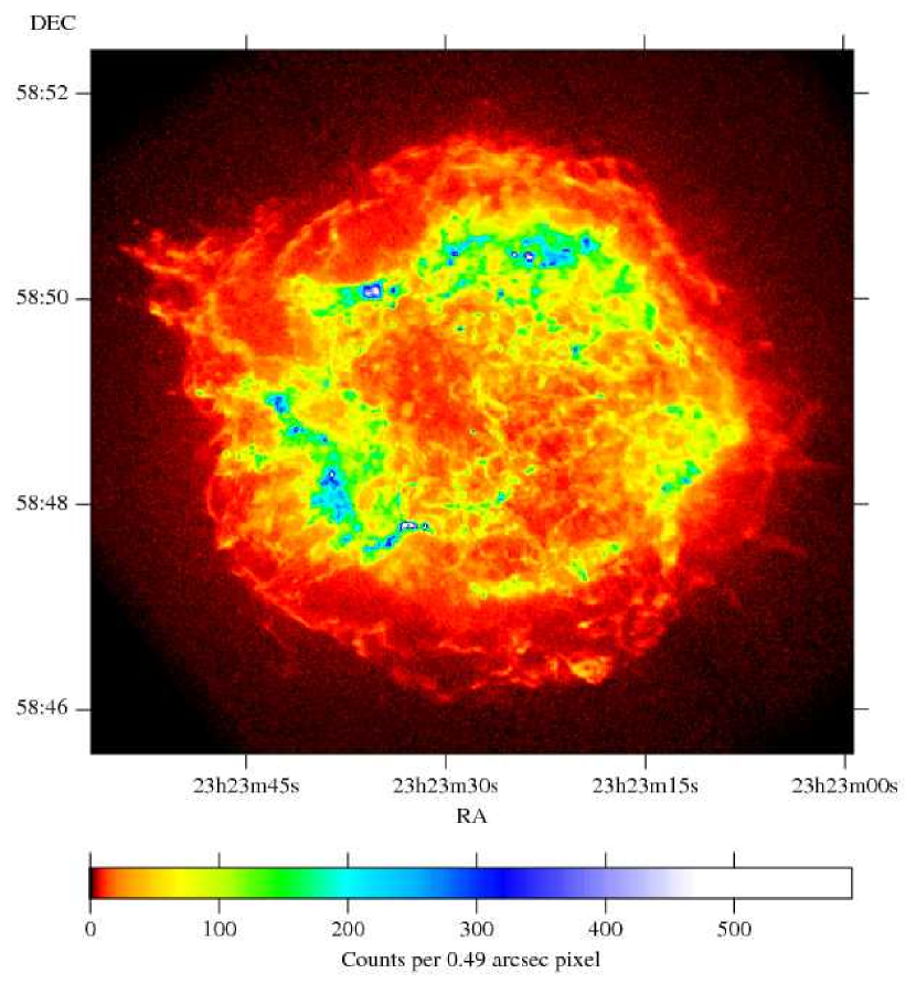
Figure 11: Background subtracted, accumulatively smoothed image of Cas A in the 0.5 to 7 keV band, smoothed using a signal-to-noise ratio threshold, $M$ of 15.

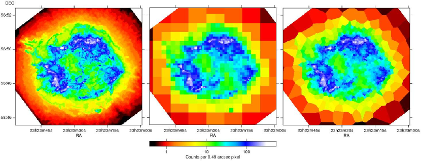
Figure 12: Binned images of Cas A. (Left) Contour binned image using a signal-to-noise binning threshold ratio, $T$, of 100. The image was smoothed using $M=15$ before binning. (Centre) Adaptively binned image with a fractional error threshold of 0.01 using algorithm of Sanders & Fabian (2001). Note that this binning did not take account of the readout background. (Right) Bin accretion binned image with a signal-to-noise of 100 using algorithm of Cappellari & Copin (2003).

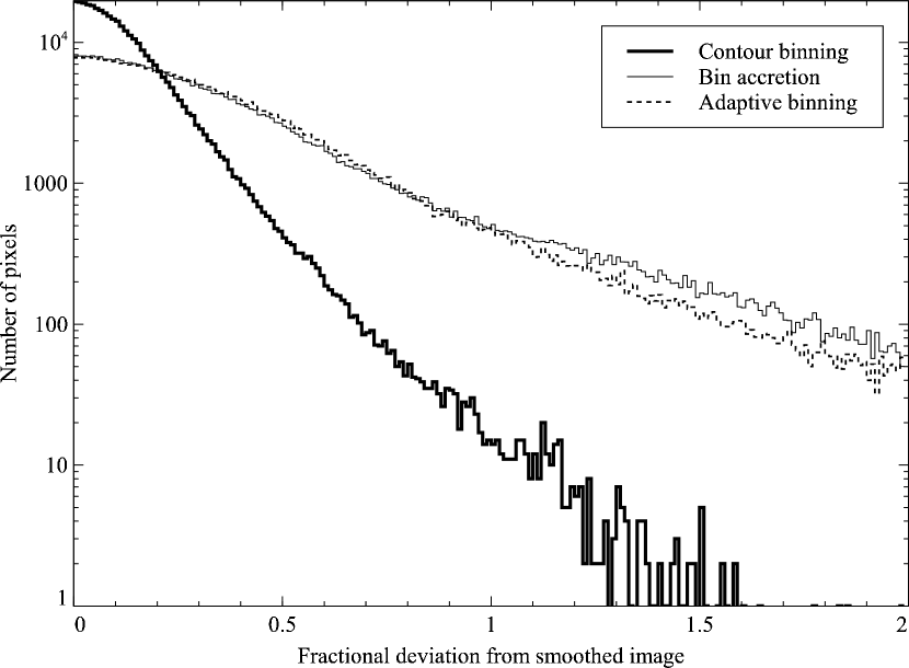
Figure 13: Histogram of fractional deviations of each pixel of a binned image from accumulatively smoothed image of Cas A (signal to noise threshold of 8). The area examined was limited to a 2.8 arcmin radius around the core of the remnant. Shown are the results for contour binning, adaptive binning and bin accretion using similar signal-to-noise ratios.

In Fig. 11 is shown an accumulatively smoothed X-ray image of the dataset. We show in Fig. 12 a contour binned image of the dataset with a signal-to-noise threshold, $T$, of 100 (the image was smoothed with a signal-to-noise threshold of 15 before binning) along with adaptively and accretion binned images with similar signal-to-noise ratios. The binning procedure created 1176 spatial bins, giving an average of $1.2\times 10^{4}$ counts per spectrum before background subtraction. It can be seen that the bins follow the shape of the surface brightness well, and better than the other binning methods. Note that there is relatively bright emission around the remnant (this is difficult to see in plots shown, due to the greyscale colour scaling). This emission is in fact radiation from Cas A scattered by dust in the interstellar medium. The measurements presented later include results outside of the remnant which are from the scattered radiation.

To compare the binning methods better, we can compare the surface brightness of binned pixels against what they are expected to be. If we take the absolute fractional difference between a binned accumulately smoothed image of the remnant and an accumulatively smoothed image, then plot the histogram of the differences, we obtain the distributions in Fig. 13. The area examined was limited to a radius of 2.8 arcmin from the centre of the remnant to avoid edge effects. The plot shows that contour binning is much better at reproducing the accumulately smoothed surface brightness of the object than the other methods. This argument assumes that an accumulative smoothed image is a good estimate of the intrinsic sky surface brightness. To make the comparison fairer we increased the signal-to-noise used by the bin accretion method to 109 to match the number of bins used by contour binning, although it makes very little difference to the results. The number of bins used by contour binning, bin accretion and adaptive binning are 1175, 1182 and 889 respectively. Contour binning also produces the most accurate surface brightnesses from our simulated data (Fig. 6). The test with the simulated data is less biased as we know the intrinsic surface brightness of the object, although the results are similar.

4.3 Spectral fitting

We extracted spectra from the events file in each of the binned regions. Rather than use the standard ciao dmextract tool we used our own code which extracts all the spectra in a single pass. The spectra were grouped to have a minimum number of 20 counts in each spectral channel using grppha from ftools. Using the ciao mkwarf and mkrmf tools, we generated weighted response and ancillary response files for each of the regions, weighted by the number of counts between 0.5 and 7 keV. In addition we extracted background spectra from the blank sky and out of time event files.

The spectra were fit using xspec 11.3.2 between energies of 0.6 and 7 keV. We fitted a vnei model to each region, with the neivers parameter set to 2.0, which uses the ionisation fractions of Mazzotta et al (1988) and uses aped (Smith et al 2001) to generate the resulting spectrum. The emission model was absorbed by a phabs absorption model (Balucinska-Church & McCammon 1992). In the fit the absorption, temperature, normalisation, ionisation timescale, redshift, Ne, Mg, Si, S, Ar, Ca, Fe and Ni abundances were free parameters (using a maximum of $40\hbox{$\thinspace\mathrm{Z}_{\odot}$}$ in each abundance parameter). The H, He, C, N and O abundances were fixed at solar values. We used the solar abundance ratios of Anders & Grevesse (1989). In some regions there are prominent lines at Fe-K energies (e.g. Hwang et al 2000), which lead to poor reduced $\chi^{2}$ values. We therefore added a Gaussian component to the model allowed to vary between 6 and 7 keV.

With the large number of free parameters it was easy for the fits to become stuck in local minima. We tried to avoid this by freeing the most influential parameters first, and doing a fit after each freeing. Also during the fit we searched for errors on the parameters to help find other $\chi^{2}$ minima. However, this prescription does not guarantee to find the absolute minimum in $\chi^{2}$ space, so some parameters may not be at their best-fitting values. In addition the best fitting parameters may not be physically sensible. After the spectra were fit, the best-fitting values of each parameter were used to generate maps.

The model used is somewhat simplistic compared to those used by other authors, not taking account of multi-temperature regions or allowing the lines from each element to have different velocities (except for Fe-K). Most of the features reported by others are reproduced, however, as we discuss below. The model also assumes the emission is thermal in origin, and does not include a non-thermal component. Hughes et al (2000) have noted continuum dominated regions. These regions can be fitted by a powerlaw component or an absorbed bremsstrahlung. Hughes et al (2000) prefer the interpretation that the continuum is X-ray synchrotron emission.

In Fig. 14 are shown the best fitting temperature, absorbing column density, ionisation timescale and velocity. The velocity was obtained by multiplying the best fitting redshift by the speed of light. Abundances for Si-like elements are shown in Fig. 15, and for Fe-like elements in Fig. 16. We finally display in Fig. 17 the normalisation of the main vnei component per unit area, the reduced-$\chi^{2}$ of the fits, the normalisation of the Gaussian Fe-K component and its energy. All the maps here have been smoothed with a Gaussian of 2 pixels (0.98 arcsec) for display purposes. The positions in the map and text are in J2000 coordinates.

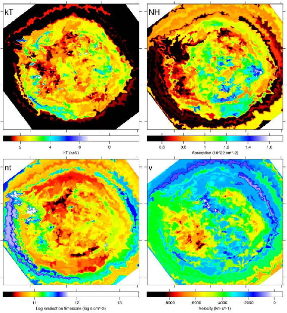
Figure 14: Temperature, absorbing column density, ionisation timescale and fitted velocity in Cas A.

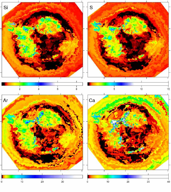
Figure 15: Abundances in Cas A of Si, S, Ar and Ca relative to solar.

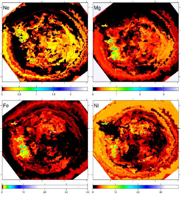
Figure 16: Abundances in Cas A of Ne, Mg, Fe and Ni relative to solar.

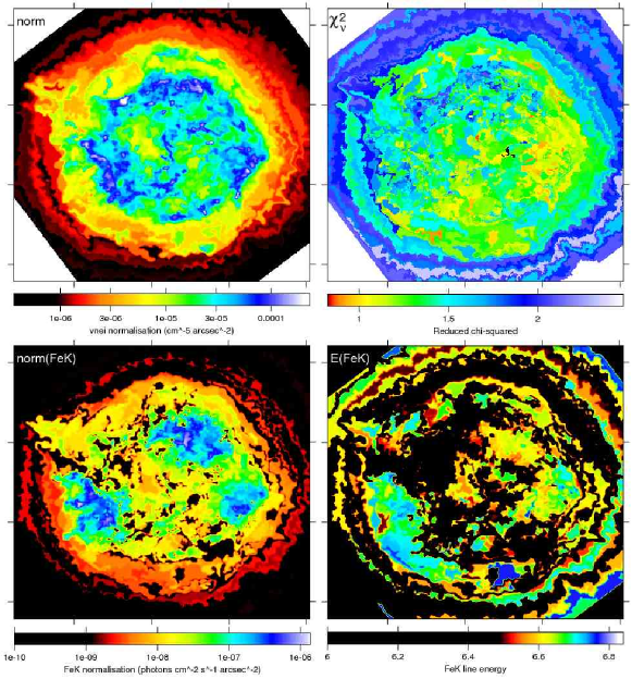
Figure 17: vnei normalisation per unit area (a proxy for the emission when the line emission has been removed), reduced $\chi^{2}$ of the fit, normalisation of the Fe-K line per unit area, and energy of the Fe-K line in Cas A.

4.4 Discussion

The absorption map (Fig. 14 [top right]) shows a dense clump of X-ray absorbing material to the west of the nebula in great detail. This material was itself found by previous observations (Keohane, Rudnick & Anderson 1996; Willingale et al 2002).

The temperature map shows the location of the inner and outer shocks well (Gotthelf et al 2001), as regions of high temperature, in addition to the direction of the north-east jet. The spectral fits also indication the position of the south-west jet (Hwang et al 2004) as higher temperature regions.

The abundance maps can be compared against those created by plotting the ratio of emission in a band crafted to the emission line of a particular element to continuum emission (Hwang, Holt & Petre 2000). This technique can only be used for elements which produce lines easily identifiable from the spectrum, however. Our maps show good agreement with the morphology of the ratio maps, although are some point-to-point differences. For example, we find more emission from S and Ar where the northern enhancement in abundance meets the eastern region, around ($23^{\mathrm{h}}33^{\mathrm{m}}33^{\mathrm{s}}$ $+48^{\circ}50^{\prime}05^{\prime\prime}$). In addition, although the Hwang et al (2000) maps show a rim of Si (and possible S) enhancement to the south of the object, we see the rim break up into separate peaks (as found in the megasecond observation of Hwang et al 2004), and see the enhancement in S, Ar, Ca, less strongly in Fe, and possibly in Mg and Ne. Again Si, S, Ar and Ca vary much more uniformly than Ne, Mg, Fe and Ni.

Although we do not allow separate velocities for the different metal components (except Fe-K), the velocity map (Fig. 14 bottom right), where velocities towards the observer are shown as negative, shows similar features to those found by others for the Si line which is usually dominant (e.g. Willingale et al 2002). We are able to map the velocity in those regions where the line emission is weak, as the emission is binned over larger regions. The absolute velocity normalisation appears to be uncertain, as earlier calibration versions with the same data gave velocities systematically around $3500\hbox{$\rm\thinspace km\rm\thinspace s^{-1}\,$}$ larger. Using the Fe-K line energy (Fig. 17 bottom right), the trend of velocity is again very similar to the Willingale et al. results, but here there is not enough signal to map the energy in low intensity regions.

The plot of the normalisation of the vnei component is particularly striking (Fig. 17 top left). It shows the emission from the remnant when the line emission has been removed. Cas A is much more symmetrical in the underlying emission.

The reduced-$\chi^{2}$ is not too bad generally when the Fe-K emission has been modelled (as it has here), given the complexity of the spectra and the simplicity of the fitted model. Where the reduced-$\chi^{2}$ is at its worst, the model seems unable to take account of the continuum and the emission lines together. Adding a second temperature component in these regions improves the quality of the fit substantially. Multiple temperature fits have been necessary before in the spectral fitting (e.g. Willingale et al 2002). There is much room for further investigation of the spectra here, but it is not the aim of this paper to study the physics of these regions in detail.

5 Conclusions

We have shown that the accumulative smoothing method, or that used by fadapt, is a robust way to estimate the real surface brightness distribution of an extended object. We have discussed the method in the cases of varying exposures, and including backgrounds.

We have described a new method for choosing regions for spectral extraction, or colour analysis, called contour binning. We have shown that method reliably creates bins which follow the surface brightness. We demonstrate the method using a simulated cluster dataset, and apply it to a Chandra observation of the supernova remnant Cassiopeia A.

The algorithm is ideal where spectral changes are associated with changes in surface brightness, as is often the case in X-ray astronomy. The results on objects with fine spatial detail are very closely matched to the object, aesthetically pleasing, and easy to interpret, compared to other methods (as exemplified by Fig. 12 and Fig. 13). As the algorithm follows the surface brightness it naturally bins regions which are likely to be physically associated. It avoids mixing spectra together for physically disassociated regions.

Availability

A C++ implementation of the algorithm can be downloaded from http://www-xray.ast.cam.ac.uk/papers/contbin/ , including other helpful associated programs.

References

- [1] Anders E., Grevesse N., 1989, Geochimica et Cosmochimica Acta, 53, 197
- [2] Arnaud, K.A., 1996, Astronomical Data Analysis Software and Systems V, eds. Jacoby G. and Barnes J., p17, ASP Conf. Series volume 101
- [3] Balucinska-Church M., McCammon D., 1992, ApJ, 400, 699
- [4] Bauer F.E., Fabian A.C., Sanders J.S., Allen S.W., Johnstone R.M., 2005, MNRAS, 359, 1481
- [5] Blanton E.L., Sarazin C.L., McNamara B.R., 2003, ApJ, 585, 227
- [6] Bourdin H., Sauvageot J.-L., Slezak E., Bijaoui A., Teyssier R., 2004, A&A, 414, 429
- [7] Cappellari M., Copin Y., 2003, MNRAS, 342, 345
- [8] Choi Y., Reynolds C.S., Heinz S., Rosenberg J.L., Perlman E.S., Yang J., 2004, ApJ, 606, 185
- [9] Diehl S., Statler T.S., 2006, MNRAS, submitted, astro-ph/0512074
- [10] Fabian A.C., Sanders J.S., Ettori S., Taylor G.B., Allen S.W., Crawford C.S., Iwasawa K., Johnstone R.M., Ogle P.M., 2000, MNRAS, 318, L65
- [11] Fabian A.C., Sanders J.S., Taylor G.B., Allen S.W., 2005, MNRAS, 360, L20
- [12] Fabian A.C., Sanders J.S., Taylor G.B., Allen S.W., Crawford C.S., Johnstone R.M., Iwasawa K., 2006, MNRAS, accepted, astro-ph/0510476
- [13] Gehrels N., 1986, ApJ, 303, 336
- [14] Gotthelf E.V., Koralesky B., Rudnick L., Jones T.W., Hwang U., Petre R., 2001, ApJ, 552, L39
- [15] Huang Z., Sarazin C., 1996, ApJ, 461, 622
- [16] Hughes J.P., Rakowski C.E., Burrows D.N., Slane P.O., 2000, ApJ, 528, L109
- [17] Hwang U., Holt S.S., Petre R., 2000, ApJ, 537, L119
- [18] Hwang U., et al., 2004, 615, L117
- [19] Johnstone R.M., Allen S.W., Fabian A.C., Sanders J.S., 2002, MNRAS, 336, 299
- [20] Keohane J.W., Rudnick L., Anderson M.C. 1996, ApJ, 466, 309
- [21] Liedahl D.A., Osterheld A.L., Goldstein W.H., 1995, ApJ, 438, L115
- [22] Markevitch M., 2004, http://hea-www.harvard.edu/~maxim/axaf/acisbg/
- [23] Markevitch M., 2003, http://hea-www.harvard.edu/~maxim/axaf/make_readout_bg
- [24] Mazzotta P., Mazzitelli G., Colafrancesco S., Vittorio N., 1998, A&AS, 133, 403
- [25] Mewe R., Gronenschild E.H.B.M., van den Oord G.H.J., 1985, A&AS, 62, 197
- [26] Peterson J.R., Jernigan J.G., Kahn S.M., 2004, ApJ, 615, 545
- [27] Sanders J.S., Fabian A.C., Allen S.W., 2000, MNRAS, 318, 733
- [28] Sanders J.S., Fabian A.C., 2001, MNRAS, 325, 178
- [29] Sanders J.S., Fabian A.C., 2002, MNRAS, 331, 273
- [30] Sanders J.S., Fabian A.C., Allen S.W., Schmidt R.W., 2004, MNRAS, 349, 952
- [31] Sanders J.S., Fabian A.C., Taylor G.B., 2005a, MNRAS, 356, 1022
- [32] Sanders J.S., Fabian A.C., Dunn R.J.H., 2005b, MNRAS, 360, 133
- [33] Smith R.K., Brickhouse N.S., Liedahl D.A., Raymond J.C., 2001a, Spectroscopic Challenges of Photoionized Plasmas, ASP Conference Series Vol. 247, eds Gary Ferland and Daniel Wolf Savin. San Francisco: Astronomical Society of the Pacific, p161
- [34] Vikhlinin A., 2003, http://asc.harvard.edu/cont-soft/software/corr_tgain.1.0.html
- [35] Willingale R., Bleeker J.A.M., van der Heyden K.J., Kaastra J.S., Vink J., 2002, 381, 1039