Constraining Primordial Non-Gaussianities from the WMAP2 2-1 Cumulant Correlator Power Spectrum

Abstract

We measure the 2-1 cumulant correlator power spectrum $C^{21}_{l}$, a degenerate bispectrum, from the second data release of the Wilkinson Microwave Anisotropy Probe (WMAP). Our high resolution measurements with SpICE span a large configuration space ($\simeq 168\times 999$) corresponding to the possible cross-correlations of the maps recorded by the different differencing assemblies. We present a novel method to recover the eigenmodes of the correspondingly large Monte Carlo covariance matrix. We examine its eigenvalue spectrum and use random matrix theory to show that the off diagonal terms are dominated by noise. We minimize the $\chi^{2}$ to obtain constraints for the non-linear coupling parameter $f_{NL}=22\pm 52\,(1\sigma)$.

1. Introduction

Quantifying the non-Gaussianity in the cosmic microwave background (CMB) puts constraints on inflationary models and possibly identifies non-linear effects from large scale structure. In addition, systematics and foregrounds might also produce non-Gaussian signatures; this possibly weakens constraints on the primordial and secondary non-Gaussianities.

A natural phenomenological parametrization of non-Gaussian models is in terms of the perturbative non-linear coupling in the primordial curvature perturbation (Komatsu & Spergel, 2001):

$$\Phi({\mathbf{x}})=\Phi_{L}({\mathbf{x}})+f_{NL}\left(\Phi^{2}_{L}({\mathbf{x}})-\left<\Phi^{2}_{L}({\mathbf{x}})\right>\right),$$ (1)

where $\Phi_{L}({\mathbf{x}})$ denotes the linear Gaussian part of the Bardeen curvature and $f_{NL}$ is the non-linear coupling parameter. The resulting leading-order non-Gaussianity is at the three-point level. Thus, the three point correlation function (e.g., Chen & Szapudi, 2005, and references therein) or its spherical harmonic transform, the bispectrum, directly estimate the leading order effect.

The bispectrum has been used extensively for studying non-Gaussianity (Komatsu et al., 2005; Creminelli et al., 2006; Medeiros & Contaldi, 2006; Liguori et al., 2006; Cabella et al., 2006). In previous measurements, the pseudo-bispectrum was used, which, like the pseudo-$C_{l}$’s, ignores in detail the effects of the complicated geometry induced by Galactic cut and cut-out holes. Pixel space statistics, such as the three-point correlation function, trivially deconvolve the geometric effects, as the convolution kernel is diagonal in pixel space. Indeed, SpICE (Szapudi et al., 2001a, Spatially Inhomogenous Correlation Estimator) uses this simple fact to estimate the angular power spectrum without explicitly inverting the $M_{ll^{\prime}}$ kernel (Hivon et al., 2002). For the bispectrum, the convolution kernel is even more complex than for the $C_{l}$’s, therefore pixel space methods are advantagous. We use the fact that the SpICE algorithm can be used to calculate (deconvolved) power spectrum of cumulant correlators $\langle{\delta T^{N}\delta T^{M}}\rangle$ (Szapudi et al., 1992). These are degenerate $N+M$-point correlation functions, and their power spectra correspond to integrated $N+M-1$ poly-spectra. In this paper we focus on the 2-1 cumulant correlator power spectrum which is directly related to bispectrum configurations. These contain less configration information than the full bispectrum, although retain more than the skewness (Komatsu et al., 2005). Note that in terms of $f_{NL}$, with near optimal weighting, the statistical power of the skewness is nearly as optimal as the full bispectrum (Komatsu et al., 2003; Spergel et al., 2006). For models with non-trivial configuration dependence, this is not the case.

We introduce the power spectrum of the 2-1 cumulant correlator together with the corresponding theoretical theoretical predictions. Statistical estimation in the data and simulations, and the theoretical calculations are are described in §3. In §4 we investigate the covariance matrix of the measurements, the $\chi^{2}$ analysis of $f_{NL}$. We summarize and discuss the work in §5.

2. power spectrum of 2-1 cumulant correlator

For the temperature fluctuation field $T(\hat{\bf n})$ in CMB, the 2-1 cumulant correlator is simply expressed as $\left<T(\hat{\bf n})^{2}T(\hat{\bf m})\right>$, where the ensemble average can be replaced by spatial (angular) average due to the assumed rotational invariance and ergodicity of the universe. Its Fourier or spherical harmonic transform corresponds to a set of summed (integrated) bispectrum configurations (Cooray, 2001):

$$C_{l}^{21}=\sum_{l_{1}l_{2}}B_{l_{1}l_{2}l}W_{l_{1}}W_{l_{2}}W_{l}\left(\begin{array}[]{ccc}l_{1}&l_{2}&l\\ 0&0&0\end{array}\right)\sqrt{(2l_{1}+1)(2l_{2}+1)\over 4\pi(2l+1)}\,.$$ (2)

Here $B_{l_{1}l_{2}l}$ is the bispectrum and $W_{l}$ is the multiple of the pixel window function and beam function of the CMB map.

The above equation can be used to turn a theoretical prediction for the full bispectrum into a prediction for the 2-1 cumulant correlator power spectrum. We follow closely the method described in Komatsu & Spergel (2001) to predict the full bispectrum using our modified version of CAMB. Then we sum the above Equation 2 in $l_{1}$ and $l_{2}$ up to $l_{i}=2000$ where $W_{l}\simeq 0.001$. Because of the linear dependency of the bispectrum on $f_{NL}$, we perform the calculation with $f_{NL}=1$.

Due to the similarity of cumulant correlators to two-point correlation functions, the analogous technique can be used for them as for measuring $C_{l}$. We use cross correlations of a triplet of maps for each measurement to avoid the uncertainties in the noise bias. The SpICE (Szapudi et al., 2001a) algorithm uses harmonic transforms to calculate fast correlation functions of two maps, and Legendre integration (Szapudi et al., 2001b) to obtain the final power spectrum. To obtain 2-1 cumulant correlators, the first two maps have to be multiplied first, as it is described next in detail. The final power spectrum can be directly compared with the theoretical prediction, as it is fully corrected for the complicated pixel geometry of the underlying maps. Our measurement is the first such bispectrum measurement, where the geometry is accurately taken into account.

3. Measurements and Predictions

We use WMAP three year coadded foreground reduced sky maps (Jarosik et al., 2006, hereafter WMAP2) with the resolution of $n_{side}=512$. There are 8 differencing assemblies differencing assemblies (DAs) for the Q, V, and W bands. We calculated the cross correlations among these 8 maps and there are $(8\times 7)/2\times 6=168$ combinations. The factor of $1/2$ is explained by the invariance of the 2-1 cumulant correlator under the exchange of the first two maps. We index the triplet of maps used in the cross-correlations by $X$ and denote the power spectrum by $C^{21}_{l}(X)$. First we prepare a “square temperature” map by multiplying pixel by pixel the first two maps in a triplet. The resulting map is cross-correlated by the third map with SpICE. We use the more conservative Kp0 mask since non-Gaussianities are expected to be more sensitive to foregrounds than the power spectrum. It takes about 330 minutes to calculate all 168 spectra on a 2 GHz class CPU for the WMAP data (or for one set of simulations). Figure 1 displays typical measurements together with theoretical predictions and simulation results for the triplet X=(Q1,Q2,V1).

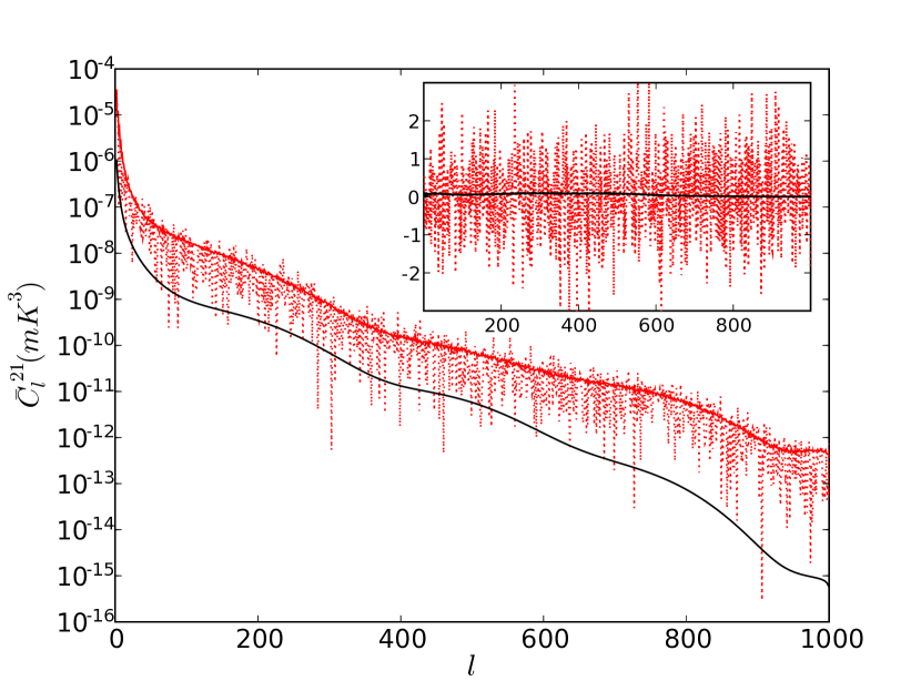
Figure 1.— A typical results of the 2-1 cumulant power spectrum normalized to the triplet $X=(Q1,Q2,V1)$. The lower solid curve is the theoretical prediction for $f_{NL}=-100$; the upper solid line is the standard deviation from 200 simulations; the dotted line corresponds to the absolute values from WMAP2. Inset: the data (without absolute value) and theory on a linear scale renormalized by the standard deviation measured from the simulations.

Qualitatively, there is no obvious sign of non-Gaussianities. To obtain accurate constraints, we estimate covariances from a set of Monte Carlo simulations and fit the $f_{NL}$ parameter. Gaussian simulations ($f_{NL}$=0) suffice, since the covariance is dominated by the Gaussian noise as long as $f_{NL}<500$ (Komatsu et al., 2003), which we already know to be true. We generated 200 simulations with SYNFAST in HEALPix package. We used the WMAP first year (WMAP1) power spectrum available from the Lambda website for input. It is the best fit $\Lambda$CDM model using a scale-dependent (running) primordial spectral index, using WMAP1, CBI and ACBAR CMB data, plus the 2dF and Lyman-alpha data. For each simulation we generate 8 DA maps closely mimicking the data (Spergel et al., 2003). These maps represent the same realization of the CMB but with different noise and beam for each. Our noise model is somewhat simplistic, and uses Gaussian realizations with standard deviation $\sigma_{0}/\sqrt{N_{obs}}$, where the effective number of observations $N_{obs}$ varies across the sky and for different DAs, and $\sigma_{0}$ is a constant for each DA. This does not take into account possible correlations in the noise, but at this writing no noise maps were available for WMAP2; our measurements in WMAP1 with more realistic noise indicate that the effects of the noise correlations are negligible on our measurement (see the last section for details). Finally, each simulation was analyzed exactly the same way as the data: we performed $33,600$ measurements in $16,00$ maps.

4. The Covariance Matrix and $\chi^{2}$ Analysis

Let us extend our notation and label our measurements and predictions for triplet $X$ as $C_{l}^{21}(X,s)$, where $s$ stands for the theory ($s=0$), one of the 200 simulations($s=1,...,200$), or the WMAP data($s=201$). Our goal is to obtain quantitative constraints for $f_{NL}$ using these results. In particular, we focus on the covariance matrix (CM).

4.1. The Covariance Matrix

The simulations can be used to obtain an experimental CM the standard way. Without any further binning, the CM is a square matrix of size $p=168\times 999=167832$ (999 stands for $l=2,...,1000$). A matrix of this size can only be inverted with supercomputers. To overcome this problem, we introduce a novel, generally applicable technique which speeds up the inversion of experimental covariance matrices. We show that the singular value decomposition (SVD) of the CM is related to another matrix of smaller size governed by the number of simulations.

Let M be the matrix where each raws and columns correspond to configurations and simulations, respectively. The SVD of this $m\times n$ matrix $M$ (the number of rows $m$ is typically larger than the number of columns $n$) is given by $M=U\Lambda V^{T}$. Here $U$ is a $m\times n$ column-orthonormal matrix, $\Lambda$ is a $n\times n$ diagonal matrix with non-negative elements, and $V$ is a $n\times n$ orthonormal matrix. In this notation the CM can be expressed as $1/nMM^{T}$. The corresponding SVD is $U(1/n\Lambda^{2})U^{T}$. This can obtain more efficiently by solving the dual problem $M^{T}M=V^{T}\Lambda^{2}V$. Once the eigenvalues and $V$ are obtained from this smaller matrix, $U=MV\Lambda^{-1}$ can be calculated. This procedure is much faster than the direct calculation of the covariance matrix, as long as $m\gg n$. Also, it is clear from the arguments, that the CM has at most $n$ non-degenerate eigenmodes. Unfortunately, using only a small number of noisy eigenmodes means that we cannot fully exploit the information content of our data. While we have performed $\chi^{2}$ analysis using the full data set, a more reliable result can be obtained by compressing the data.

4.2. Binning

It would be desirable to combine different measurements of the same $l$ with inverse variance weighting to compress our data set. Such a combination for the angular power spectrum is nearly optimal (Fosalba & Szapudi, 2004). The generalization is a bit more complex, since the pixel and beam window functions for a particular triplet in Equation 2 cannot be decomposed, therefore one cannot simply obtain corrected $C^{21}_{l}$ estimates independent of window functions.

To overcome this problem we introduce a new unbiased quantity,

$$\widetilde{C}_{l}^{21}(X,s)=C_{l}^{21}(X,s)\times\frac{C_{l}^{21}((V1,V2,Q1),0)}{C_{l}^{21}(X,0)}\Big{|}_{f_{\rm NL}=1},$$ (3)

the cumulant correlator power spectrum normalized according to the theory to a arbitrary triplet $X=(V1,V2,Q1)$ at a fiducial value $f_{NL}=1$. In this normalization the window factors approximately cancel, therefore we can obtain an inverse variance weighted

$$\bar{C}^{21}_{l}(s)=\frac{\sum_{X=1}^{168}w(X)\widetilde{C}_{l}^{21}(X,s)}{\sum_{X=1}^{168}w(X)},$$ (4)

where $w(x)$ is proportional to the inverse variance measured in the simulations. The advantage of the inverse variance weighting over the noisy covariance matrix is that each weight is determined with high accuracy $1/\sqrt{200}\simeq 0.07$, while, as we will see, modes of the matrix are significantly affected by the noise. Therefore, although our numerical method of the previous section allows us to handle a matrix of very large size, we opted for the inverse variance weighted estimators to suppress the noise more effectively.

4.3. Random Matrix Theory

To assess the level of noise in our final covariance matrix, we use some results from random matrix theory. (e.g., Sengupta & Mitra, 1999; Laloux et al., 1999). As before, let us assume that a CM $C$ is constructed as $C=1/nMM^{T}$, from $M$, an $m\times n$ rectangular matrix. Let us further assume that $M$ is composed of independent, identically distributed random variables with zero mean and unit variance. In the limit $m\to\infty$, $n\to\infty$ while $Q=n/m$ is kept fixed, the eigenvalue spectrum will tend to:

$$\rho_{C}(\lambda) = \frac{Q}{2\pi}\frac{\sqrt{(\lambda_{max}-\lambda)(\lambda-\lambda_{min})}}{\lambda},$$ (5)

$$\lambda_{min}^{max} = 1+1/Q\pm 2\sqrt{1/Q},$$ (6)

with $\lambda\in[\lambda_{min},\lambda_{max}]$. The eigenvalue density of $C$, $\rho_{C}(\lambda)$ is defined as

$$\rho_{C}(\lambda)=\frac{1}{m}\frac{dn(\lambda)}{d\lambda},$$ (7)

where $n(\lambda)$ is the number of eigenvalues of $C$ less than $\lambda$.

In our numerical construction of the covariance matrix, if $\bar{C}^{21}_{l}$were independent of each other, we would have a random matrix. How significant are the correlations? According to Figure 2, the density of eigenvalues of our CM appears to be consistent with the random matrix theory with $Q=999/200$, with possibly a slight deviation for the largest eigenvalues. Comparing with random matrix simulations, we find that $Q=950/200$ would produce the same effect. While we keep $Q=999/200$ in our analysis, this might be a sign of small correlations in the CM at the $5\%$ level; this could effect our final $\chi^{2}$ and our final error-bars only slightly.

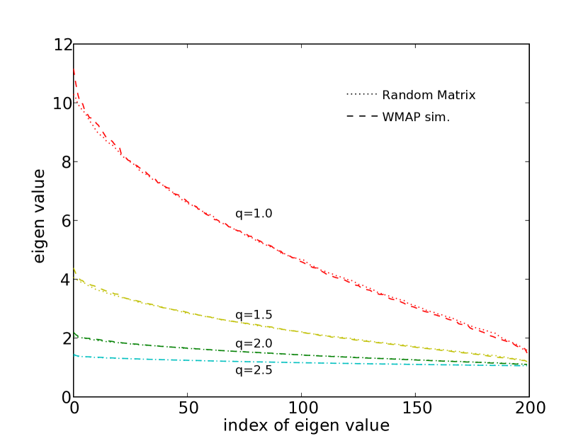
Figure 2.— The eigenvalue spectrum for a set of power mapped CMs from 200 WMAP2 simulations and from the 200 random matrix simulations. The original matrix corresponds to $q=1$. To display more detail, we plot unbinned (sorted) eigenvalues of our CM along with those obtained from random matrix simulations. The spectacular agreement indicates that the random matrix assumption is fairly accurate.

To further investigate the randomness of the covariance matrix, we apply the technique of power mapping to our CM and random matrix simulations for comparison. The $q$th power mapping of a matrix $C$ is defined as(Guhr & Kälber, 2003):

$$C_{kl}^{(q)}=\mathrm{sign}(C_{kl})|C_{kl}|^{q}.$$ (8)

Guhr & Kälber (2003) show that the eigenvalue spectral density of power mapped correlation matrices can detect correlations otherwise buried in the noise. The variance of individual elements scales as $1/n^{q/2}$, i.e. effective number of simulations increased to $n^{q}$ by power mapping. In our case, no significant deviation from random matrix theory appears as a result of power mapping (see Figure 2), which shows that the covariance is dominated by random noise.

5. Results and Discussion

Given that the CM of our measurement is consistent with the random matrix assumption at the 5% level, and that from 200 Monte Carlo simulations 7% fluctuations are expected for each of its elements, we conclude that it is consistent with our simulations to use a diagonal $\chi^{2}$ rather than weighting with the noisy off diagonal elements of CM. We found that using diagonal $\chi^{2}$ is entirely robust when we vary our binning scheme or apply no binning. On the contrary, using the noisy eigenmodes of the CM produces somewhat unstable results.

Minimizing $\chi^{2}$ as function of $f_{NL}$ gives $f_{NL}=22\pm 52\,(1\sigma)$, which is the final result of our paper. The minimum reduced $\chi^{2}$ is about 1.1 for 998 degrees of freedom. According to our discussion §4.3 there might be an additional $5\%$ uncertainty on these results because we neglected off diagonal correlations. Our results are entirely consistent with Spergel et al. (2006) despite that we did not weight with the theory. The lack of optimal weighting is compensated by the increased configuration dependence of our statistic. Note that we did not attempt to correct for point source contamination, but this should have a negligible effect on our results (Spergel et al., 2006).

To test the robustness of our constraints, we divided the 200 simulations to two sets of 100 simulations, then repeated the full statistical analysis with each set. We found consistent results: $f_{NL}=24\pm 54$ and $f_{NL}=21\pm 49$, respectively.

To test the degree to which noise correlations might affect our covariance, we also repeated our analysis of the CM with the WMAP1 simulations of Chen & Szapudi (2005). where the correlated noise were used. The eigenvalue spectrum is virtually identical to what we get for WMAP2 simulations.

Finally, we repeated our analysis using the less conservative Kp2 mask and obtained $f_{NL}=-78\pm 52$. This shows that the statistical variance of our results is already of the same order of magnitude as the possible effect of foreground corrections near the galactic plane (Spergel et al., 2006), therefore it would be difficult to improve on significantly with the present data set.

We acknowledge useful discussions with Adrian Pope and Mark Neyrinck. Some of the results in this paper have been derived using the HEALPix (Górski et al., 2005) package. We acknowledge the use of the Legacy Archive for Microwave Background Data Analysis (LAMBDA). Support for LAMBDA is provided by the NASA Office of Space Science. The authors gratefully acknowledge support by NASA through AISR NAG5-11996, NNGO06GE71G and ATP NASA NAG5-12101 as well as by NSF grants AST02-06243, AST-0434413 and ITR 1120201-128440.

References

- Cabella et al. (2006) Cabella, P., Hansen, F. K., Liguori, M., Marinucci, D., Matarrese, S., Moscardini, L., & Vittorio, N. 2006, MNRAS, 497
- Chen & Szapudi (2005) Chen, G. & Szapudi, I. 2005, ApJ, 635, 743
- Cooray (2001) Cooray, A. 2001, Phys. Rev. D, 64, 043516
- Creminelli et al. (2006) Creminelli, P., Nicolis, A., Senatore, L., Tegmark, M., & Zaldarriaga, M. 2006, Journal of Cosmology and Astro-Particle Physics, 5, 4
- Fosalba & Szapudi (2004) Fosalba, P. & Szapudi, I. 2004, ApJ, 617, L95
- Górski et al. (2005) Górski, K. M., Hivon, E., Banday, A. J., Wandelt, B. D., Hansen, F. K., Reinecke, M., & Bartelmann, M. 2005, ApJ, 622, 759
- Guhr & Kälber (2003) Guhr, T. & Kälber, B. 2003, Journal of Physics A Mathematical General, 36, 3009
- Hivon et al. (2002) Hivon, E., Górski, K. M., Netterfield, C. B., Crill, B. P., Prunet, S., & Hansen, F. 2002, ApJ, 567, 2
- Jarosik et al. (2006) Jarosik, N., Barnes, C., Greason, M. R., Hill, R. S., Nolta, M. R., Odegard, N., Weiland, J. L., Bean, R., Bennett, C. L., Dore’, O., Halpern, M., Hinshaw, G., Kogut, A., Komatsu, E., Limon, M., Meyer, S. S., Page, L., Spergel, D. N., Tucker, G. S., Wollack, E., & Wright, E. L. 2006, ArXiv Astrophysics e-prints
- Komatsu et al. (2003) Komatsu, E., Kogut, A., Nolta, M. R., Bennett, C. L., Halpern, M., Hinshaw, G., Jarosik, N., Limon, M., Meyer, S. S., Page, L., Spergel, D. N., Tucker, G. S., Verde, L., Wollack, E., & Wright, E. L. 2003, ApJS, 148, 119
- Komatsu & Spergel (2001) Komatsu, E. & Spergel, D. N. 2001, Phys. Rev. D, 63, 063002
- Komatsu et al. (2005) Komatsu, E., Spergel, D. N., & Wandelt, B. D. 2005, ApJ, 634, 14
- Laloux et al. (1999) Laloux, L., Cizeau, P., Bouchaud, J.-P., & Potters, M. 1999, Physical Review Letters, 83, 1467
- Liguori et al. (2006) Liguori, M., Hansen, F. K., Komatsu, E., Matarrese, S., & Riotto, A. 2006, Phys. Rev. D, 73, 043505
- Medeiros & Contaldi (2006) Medeiros, J. & Contaldi, C. R. 2006, MNRAS, 367, 39
- Sengupta & Mitra (1999) Sengupta, A. M. & Mitra, P. P. 1999, Phys. Rev. E, 60, 3389
- Spergel et al. (2006) Spergel, D. N., Bean, R., Dore’, O., Nolta, M. R., Bennett, C. L., Hinshaw, G., Jarosik, N., Komatsu, E., Page, L., Peiris, H. V., Verde, L., Barnes, C., Halpern, M., Hill, R. S., Kogut, A., Limon, M., Meyer, S. S., Odegard, N., Tucker, G. S., Weiland, J. L., Wollack, E., & Wright, E. L. 2006, ArXiv Astrophysics e-prints
- Spergel et al. (2003) Spergel, D. N., Verde, L., Peiris, H. V., Komatsu, E., Nolta, M. R., Bennett, C. L., Halpern, M., Hinshaw, G., Jarosik, N., Kogut, A., Limon, M., Meyer, S. S., Page, L., Tucker, G. S., Weiland, J. L., Wollack, E., & Wright, E. L. 2003, ApJS, 148, 175
- Szapudi et al. (2001a) Szapudi, I., Prunet, S., & Colombi, S. 2001a, ApJ, 561, L11
- Szapudi et al. (2001b) Szapudi, I., Prunet, S., Pogosyan, D., Szalay, A. S., & Bond, J. R. 2001b, ApJ, 548, L115
- Szapudi et al. (1992) Szapudi, I., Szalay, A. S., & Boschan, P. 1992, ApJ, 390, 350